HAL Id: hal-01291347
https://hal-enpc.archives-ouvertes.fr/hal-01291347v2
Preprint submitted on 25 Mar 2016HAL is a multi-disciplinary open access archive for the deposit and dissemination of sci-entific research documents, whether they are pub-lished or not. The documents may come from
L’archive ouverte pluridisciplinaire HAL, est destinée au dépôt et à la diffusion de documents scientifiques de niveau recherche, publiés ou non, émanant des établissements d’enseignement et de
Generalized entropy models
Mogens Fosgerau, André de Palma
To cite this version:
Generalized entropy models
Mogens Fosgerau
André de Palma
yMarch 23, 2016
Abstract
We formulate a family of direct utility functions for the consumption of a differentiated good. This family is based on a generalization of the Shan-non entropy. It includes dual representations of all additive random utility discrete choice models, as well as models in which goods are complements. Demand models for market shares can be estimated by plain regression, en-abling the use of instrumental variables. Models for microdata can be esti-mated by maximum likelihood.
Keywords: market shares; product differentiation; discrete choice; duality; generalized entropy
JEL: D01, C25, L1
Technical University of Denmark, Denmark, [email protected]
yCES, ENS Cachan, CNRS, Université Paris-Saclay, Cachan, France, and CECO, Ecole Poly-technique, [email protected].
1
Introduction
We construct a family of direct utility functions that describe consumer demand for one unit of a differentiated good. A consumer with income y and consumption
q = (q1; :::; qJ) of the differentiated good has utility u (q; y) = y + q v +
(q), where > 0 and v = (a p) is quality minus price in utility units.
The function belongs to a family of generalized entropies, defined through a number of conditions as a generalization of the Shannon (1948) entropy; it is a concave function that expresses taste for variety while leading to a tractable link between consumption and utility. We find a new general structure for generalized entropy, which enables us to provide rules for constructing generalized entropies and a range of specific examples showing that generalized entropy may be used to generate rich patterns of substitution and complementarity.
We share the idea of using convex analysis and duality in a discrete choice context with other recent contributions. Salanié and Galichon (2015) consider matching models with transferable utility and arrive at a generalization of entropy that belongs to our family of generalized entropies. Chiong et al. (2015) apply similar ideas to dynamic discrete choice models. Melo (2012) uses duality to show existence of a representative agent for a dynamic discrete choice model on a network. The essential contribution of this paper is the finding that generalized entropy has a certain structure that allows us to access a new and rich universe of tractable demand models that has not been explored before.
Models specified in terms of generalized entropy may be estimated using sim-ple regression with instruments that are available within the model. In this respect, our paper is closely related to Berry(1994) andBerry and Haile (2014) who in-vert the market shares of an additive random utility model (ARUM) to find cor-responding utility levels. Given that this transformation is known, Berry(1994) shows how model parameters may be estimated using standard instrumental vari-able regression techniques with inverted markets shares as dependent varivari-ables. Inversion of market shares may be carried out with an explicit formula for the case of the multinomial and the nested logit models. However, these models imply substitution patterns that may be implausible in many applications (Berry et al.,
pa-rameter models, but then numerical methods are necessary to carry out the Berry inversion, which leads to numerical and computational issues in combination with the random parameters (Knittel and Metaxoglou,2014).
In this paper we formulate models, not in the space of indirect utilities of dis-crete choice models, but in the dual space of consumption shares. This makes the inverted market shares directly available and numerical methods are unnec-essary for computing them. Consistency with maximization of a well-behaved utility function is automatically ensured. We provide a range of examples leading to substitution and complementarity patterns that go well beyond the nested logit example. These may potentially be used as alternatives to the random coefficient logit in what has become known as Berry, Levinsohn, Pakes or just BLP models (Berry et al.,1995).
Our generalized entropy models can also be applied to microdata of discrete choices, allowing individual level information to be taken into account. In this case, numerical methods are required to compute the likelihood. The likelihood can be computed via a fixed point iteration that we show is guaranteed to converge in a range of circumstances. Then models can be estimated using maximum likeli-hood. Random parameters are not required to allow for more complex substitution patterns than plain or nested logit.
The family of models based on generalized entropy is large: we show that it comprises models corresponding to any ARUM. For the multinomial logit model, the corresponding generalized entropy is the Shannon entropy (Anderson et al.,
1988). The generalized entropy family is in fact larger than the family of ARUM, we show that generalized entropies exist that lead to demands that are not consis-tent with any ARUM. Importantly, generalized entropy models exist where goods may be complements rather than substitutes, whereas goods are always substitutes in ARUM.
McFadden(1978) developed a family of discrete choice models based on the form of the expected maximum utility function when random utilities follow a multivariate extreme value (MEV) distribution. This family includes the multino-mial and the nested logit models as the simplest special cases. McFadden(1978) applied a nesting device to utilities to create a range of instances of MEV mod-els; in the present paper we create instances of generalized entropy models by
applying a nesting device to market shares.
Fudenberg et al.(2014) analyzes utility of the same form as used in this paper, but where the entropy term (q) is separable as a sum of terms fj(qj). It is crucial
for the results in this paper not to require such separability. Mattsson and Weibull
(2002) have a similar setup, but where (q) is interpreted as an implementation
cost and where axioms are imposed that essentially reduce (q) to the Shannon
entropy such that demand arises that is consistent with the logit model. This paper uses generalized entropy to describe substitution and complementarity patterns that go well beyond this.
The budget set for the consumer in this paper incorporates a quantity con-straint and is hence not linear in income and prices. This fits into the framework ofFosgerau and McFadden(2012) who develop a micro-economic theory of con-sumer demand under general budgets and where utility is perturbed by a linear term such as q v.
Section2introduces generalized entropy and uses it to define and solve a class of direct utility models for market shares. A range of results and accompanying examples are presented that allows members of this class to be constructed. Sec-tion3shows how utility parameters in generalized entropy models may be recov-ered from market level data using standard regression techniques. Section 4 re-lates generalized entropy to discrete choice models and shows that all ARUM are represented by generalized entropy via duality. Section4.1 presents a fixed point iteration that converges to the probability vector associated with utility levels v in a discrete choice setting and applies this in an example of maximum likelihood estimation using microdata of discrete choices. Section 5concludes. Proofs are in the appendix.
2
Direct utility models for market shares
2.1
Notational conventions
Vectors are denoted simply as q = (q1; :::; qJ). A univariate function applied to
a vector is understood as coordinate-wise application of the function, e.g., eq = (eq1; :::; eqJ). Consequently, if a is a real number then a + q = (a + q
The multivariate function S : RJ ! RJ is composed of univariate functions with superscripts (j): S (q) = S(1)(q) ; :::; S(J )(q) . Subscripts denote partial
derivatives, e.g. Gj(v) = @G(v)@v
j . The gradient with respect to a vector v is rv;
e.g., for v = (v1; :::; vJ),rvG (v) = @G(v)@v1 ; :::;@G(v)@v
J . The Jacobian is denoted
J with, for example,
Jln S(q) = 0 B @ @ ln S(1) @q1 ::: @ ln S(1) @qJ ::: ::: ::: @ ln S(J ) @q1 ::: @ ln S(J ) @qJ 1 C A :
A dot indicates an inner product or products of vectors and matrixes. The unit simplex in RJ is . A subset g
f1; :::; Jg is called a nest and we use the
notation qg =
P
j2g
qj as shorthand for the sum of q over a nest g.
2.2
Consumer demand
Consider a consumer with income y facing a price vector p for J varieties of a differentiated good and a numeraire good with price 1. The consumer maximizes utility z + q a + (q), where > 0, q is the vector of quantities of the
differ-entiated good, and z is the quantity of the numeraire good. The consumer has a budget constraint y z + q p. Importantly, the consumer also has a quantity
con-straintPjqj = 1, which normalizes demand for the differentiated good. Income
is sufficiently large, y > maxjfpjg, that consumption of the numeraire good is
always positive. The budget constraint is always binding and substituting it into utility leads to
u (q; y) = y + q v + (q) ; (1)
where v = (a p).
We begin by giving an abstract formulation of ; specific examples will be provided afterwards. Generalized entropy is a function : [0;1)J ! R[ f 1g
given by
(q) = (
q ln S (q) ; q2
1; q =2 ; (2)
Note that the domain of generalized entropy embodies the constraint that demands
qj sum to 1.1
A function S is a flexible generator if it satisfies the following four conditions.
Condition 1 S is continuous, and homogenous of degree 1.
Condition 2 is concave.
Condition 3 S is differentiable at any q 2 relint ( ) with
J X j=1 qj @ ln S(j)(q) @qk = ; k 2 f1; :::; Jg ; where > 0.
Condition 4 S is globally invertible.
In order to build intuition, let us consider what happens if the components S(j)
of a flexible generator are identical and, as in Fudenberg et al. (2014), each S(j) depends only on qj. Then Condition3, which may be expressed as q Jln S(q) =
(1; :::; 1), reduces to @ ln S(j)(qj)
@qj = =qj, which implies that S
(j)(q
j) = cqj, for
some c > 0. The function S (q) = cq satisfies Conditions1-4and the correspond-ing generalized entropy (q) = q ln q ln c is just the Shannon entropy up to
a constant. Maximizing utility (1) with this entropy under the quantity constraint
P
jqj = 1 leads to logit demand (Anderson et al.,1988)
q (v) = e v1 PJ j=1evj ; :::; e vJ PJ j=1evj ! :
In general, each S(j)depends on the whole vector q, which complicates the deriva-tion of an expression for the demand. Here Condideriva-tion3plays a key role, ensuring that @ (q) =@qk = ln S(k)(q) + . This leads to a tractable and familiar form
for demand as shown in the next theorem.
1We will show (Theorem4) that the convex conjugate of the ARUM surplus function has this
Theorem 1 Let be a generalized entropy as given in (2). Maximization of utility u (q; y) = y + q v + (q) leads to a demand system with interior solution
q (v) = H (1)(ev) PJ j=1H(j)(ev) ; :::; H (J )(ev) PJ j=1H(j)(ev) ! ; (3) where H = S 1.
Demand q corresponds to v in the expression (3) if and only if v and q are related through the flexible generator S by v = ln S (q) + c for some c2 R.
As we have seen, the form (3) of demand generalizes the logit demand. We shall establish in Section4that for any ARUM there exists a generalized entropy that leads to the same demand. We shall also show in Theorem2that generalized entropies exist that are not consistent with ARUM demand.
The second part of Theorem1establishes that utility can be computed up to a constant directly from demand, given a flexible generator S. This result is used in Section3, which discusses estimation of these models via regression.
Throughout the paper, we denote the inverse of a flexible generator S by H
S 1. The formulation of generalized entropy does not rule out corner solutions in
general. Whether zero demands can arise depends on the specific formulation of generalized entropy.
We end this section by a proposition, proved in Fosgerau and McFadden
(2012)2, showing that each demand q
j is weakly increasing as a function of the
corresponding vj. More generally, it establishes a cyclical monotonicity condition
(Rockafellar, 1970, chap. 24) which guarantees that demand is contained in the subdifferential of a convex function.
Proposition 1 (Cyclical monotonicity) If vk K+11 ; K 1 is a finite sequence of vectors with vK+1 = v1, and demand q is as described in Theorem1, then
K
P
k=1
vk+1 vk q vk 0: (4)
Each demand function qj(v) is weakly increasing in vj; j = 1; :::; J .
We proceed to construct instances of generalized entropy for applications.
2.3
Construction of generalized entropies
We have already identified one flexible generator, namely the identity S (q) = q. The following subsections provide ways to generate many more flexible genera-tors. An obstacle that we will face is to establish invertibility of candidate flexi-ble generators. To overcome this, we have the following lemma, adapted from a global inversion theorem for homogeneous nonlinear maps.
Lemma 1 (Ruzhansky and Sugimoto 2014) Let J 3 and let S: (0;1)J ! (0;1)J be continuously differentiable, linearly homogenous with a Jacobian de-terminant that never vanishes and with infq2 kS (q)k > 0. Then S is invertible.
In the examples below we will see ways to construct functions that satisfy Conditions 1-3. In order for these functions to be flexible generators, it then re-mains to ensure that they are invertible. Building on Lemma 1, the next lemma establishes conditions under which the weighted geometric average of such func-tions, where just one of them must itself be a flexible generator, leads to a new flexible generator.
Lemma 2 (Averaging) Let T1; :::; TK : (0;1)J ! (0; 1)J satisfy Conditions
1-3, where the Jacobian of each ln Tkis symmetric and positive semidefinite and
positive definite for at least one k. If Tk(j)(q) qj for each k and j and 1; :::; K
are positive numbers that sum to 1, then S: (0;1)J ! (0; 1)J given by
S = K Q k=1 T k k is a flexible generator.
As a consequence, a mapping created by averaging the identity T1(q) = q with
some T2 that satisfies the conditions of the lemma except positive definiteness is
always invertible and hence it is a flexible generator.
Proposition 2 presents a general construction of flexible generators through a nesting operation. A nest g is a set of goods for which a term q g
3 1 2 4 5 6 7 g1 g2 g3 g4 g5 g6 g7 8 9
Figure 1: Nesting example with 9 goods and 7 nests.
entropy component of utility, where g 2 ]0; 1] is a nesting parameter. The closer
g is to 1, the more the goods in nest g act in the utility as one single good and
they become closer to being perfect substitutes. The division of alternatives into nests is illustrated in Figure 1. As the figure shows, one alternative may belong in several nests, and nests may or may not be subsets of other nests. Proposition
2 requires that the nesting parameters sum to 1, summed across the nests that contain any given of the J goods.3
Proposition 2 (General nesting) Let G 2f1;:::;Jg be a finite set of nests with
associated nesting parameters g, wherePfg2Gjj2gg g = 1 for all j and g > 0
for all g 2 G. Let S = S(1); :::; S(J ) be given by
S(j)(q) = Y
fg2Gjj2gg
q g
g : (5)
3In the example this may achieved by letting
1 = 3= 6 = > 0 and 2 = 4 = 5 = 7= 1 > 0.
Then S satisfies Conditions 1-3, the Jacobian of ln S is symmetric and positive semidefinite, and for each j, S(j)(q) qj. If the Jacobian of ln S is positive
definite, then S has an inverse and S is a flexible generator.
The following examples illustrate the application of Proposition2to construct a flexible generator.
Example 1 Consider J 3 with all possible nests with 1 or 2 alternatives as elements, e.g. for J = 3:
G = ff1g ; f2g ; f3g ; f1; 2g ; f1; 3g ; f2; 3gg :
Each alternative belongs to J nests and we let g = 1=J . Define in accordance with (5) the function S by
S(j)(q) = q 1 J j Y i6=j (qi+ qj) 1 J :
By Proposition2this is a flexible generator. The demand solves S (q) = ev cfor some c2 R.
The next example shows that Proposition2leads to the nested logit model as a special case.
Example 2 Partition the set of alternativesf1; :::; Jg into nests g 2 G and denote
by gj the nest that contains alternative j. Let
S(j)(q) = qjgjqg1j gj; j 2 gj; (6)
where gj 2]0; 1] are parameters. Then S is a flexible generator by Proposition2. It is straightforward to verify that the equation S (~q) = ev has solution
~ qj = e vj gj 0 @X i2gj e vi gj 1 A gj 1 :
Normalizing the sum of demands to 1 leads to qj = ~ qj P g2Gq~g = e vj gj P i2gje vi gj e gj ln Pi2gje vi gj ! P g2Ge gln P i2ge vi g !;
which is the nested logit model (McFadden,1978).4
We shall now use the general nesting result of Proposition2to create a cross-nested model, which generalizes the cross-nested logit model. Say that a set of products can be naturally grouped according to two criteria, where one grouping is not a subdivision of the other. For example, automobiles may be grouped according to brand or according to body type. We shall create a structure that is similar to the nested logit model, but which, unlike the nested logit model, allows for non-nested groupings.5 In this example, we also include an outside good, with index
zero.
Example 3 Let 0; 1; 2 > 0, 0+ 1+ 2 = 1. Let c(j) be the set of products
that are grouped together with product j on criteria c = 1; 2. Denote as before q c(j)=Pi2 c(j)qi and define S by S(j)(q) = ( q0; j = 0 q 0 j q 1 1(j)q 2 2(j); j > 0: (7)
Then it follows directly from Proposition 2 that S is a flexible generator. The cross-nesting model is applied in Section3.1.
The next proposition provides a case that goes beyond averaging of simple nesting flexible generators and where the inversion of market shares can be carried out to yield a closed form expression for demand.
4Berry (1994) noticed the explicit inversion of the nested logit demand and used inversion
of market shares to estimate utility parameters using standard regression techniques. Verboven
(1996) used the same inversion when deriving nested logit demand for a representative consumer.
5With only the nested logit model available, researchers have been forced to choose a hierarchy
of criteria, for example first grouping cars by make and then by body type within each make. With cross-nesting, it is not necessary to fix such hierarchy.
Proposition 3 (Invertible nesting) Let S be given by (5), where the number of nests is equal to the number of alternatives. Let W = diag g1; ::; g
J be a
diagonal matrix of positive nesting parameters and let MJ J = 1fj2gg be an
incidence matrix, where rows correspond to alternatives and columns correspond to nests. Suppose that M is invertible. Then S has an inverse and S is a flexible generator. Moreover, unnormalized demand satisfies
v = ln S (~q), ~q = M> 1exp W 1M 1v :
The next example illustrates the application of Proposition3.
Example 4 Consider J 3 and define nests from the symmetric incidence matrix M with entries Mij = 1fi6=jg. Then each alternative is in J 1 nests and we may
associate weights g = 1= (J 1) with each nest. The inverse of the incidence matrix has entries (M 1)ij = J11 1fi=jg. Solving ln S (~q) = v leads to ~q = M 1exp [(J 1) M 1v],or equivalently
~ qi = J X j=1 1 J 1 1fi=jg exp J X k=1 1 (J 1) 1fk=jg vk ! = J X j=1 1 J 1 1fi=jg exp J X k=1 vk ! e (J 1)vj = exp J X k=1 vk ! 1 J 1 J X j=1 e (J 1)vj e (J 1)vi ! :
Normalized demand is then
qi = PJ j=1e (J 1)vj (J 1) e (J 1)vi PJ j=1e (J 1)vj :
The model in the previous example looks similar to the multinomial logit but is different in important ways. First, it does not have the independence from irrelevant alternatives property. Second, zero demands may arise.6 The above expression for demand leads to non-negative demands only for values of v within
some set. A way to ensure that demands are strictly positive is to average with a flexible generator such as the simple identity, since then ln qj must all be finite.
Third, the demand from the invertible nesting model in the example is not consistent with any ARUM. ARUM demand has the restrictive feature that the mixed partial derivatives of qj alternate in sign (McFadden,1981). This feature is
not exhibited by the demand generated in this example, since@q1
@v2 < 0,
@2q 1
@v2@v3 < 0.
7
Thus, we have established the following theorem.
Theorem 2 Some generalized entropies lead to demand systems that cannot be
rationalized by any ARUM.
In Section4we establish that all ARUM have a generalized entropy as coun-terpart that leads to the same demand. Thus the class of generalized entropies is strictly larger than the class of ARUM models.
The signs of the mixed partial derivatives of a quantity with respect to the prices of other goods vary in the same way also for CES demand under the stan-dard linear budget constraint when CES utility is u (x) = PJj=1 jxj; j > 0; 2
(0; 1). It is thus possible for a well-behaved utility function that the signs of the
mixed partial derivatives of qj are not consistent with those predicated by ARUM.
Consider now a pair ; S of generalized entropy and flexible generator. If A
is a J J permutation matrix, then q ! (Aq) is also a generalized entropy,
since application of a permutation matrix to q just amounts to a reordering of the dimensions of q. The convex hull of the set of J J permutation matrixes is the set
of J J doubly stochastic matrixes, i.e. matrixes with non-negative elements that
sum to 1 across rows and columns (Birkhoff,1946;Mirsky, 1958) The following proposition shows more generally how a flexible generator can be transformed into a new flexible generator by a location shift and a matrix with non-negative entries that sum to 1 across columns.
7Note that @q1 @v2 (J 1) 2 e (J 1)(v1+v2) < 0 and @2q1 @v2@v3 2 (J 1)3e (J 1)(v1+v2+v3)< 0.
Proposition 4 (Transformation) Let T be a flexible generator, m 2 RJ; and let A =faijg 2 RJ RJ be invertible with aij 0 andP
i
aij = 1. Then
S : q ! exp A>[ln (T (Aq))] + m (8)
is a flexible generator.
We shall illustrate Proposition4with a flexible generator that leads to demand where goods may be complements in the sense that the demand for one good increases as the utility component vj of another good increases.
Example 5 Let J = 3 and define
A = 0 B @ :4 :6 0 :6 :4 0 0 0 1 1 C A :
Compute demand according to Proposition4with m = 0 to find that
~ q = A 1 exph A> 1vi = 0 B @ 3e3v1 2v2 2e3v2 2v1 3e3v2 2v1 2e3v1 2v2 ev3 1 C A ; which leads to q3 = e v3 e3v2 2v1+e3v1 2v2+ev3. Then @q3 @v1 > 0 iff v2 v1 > 1 5ln 3 2.
Goods are always substitutes in an ARUM. Complementarity is, however, im-portant for describing situations where some goods tend to be bought together, for example taco chips and salsa. The example above establishes that generalized entropy models are able to allow goods to be complements. We state this insight as a theorem and note that this is also another example of a generalized entropy model that is not consistent with any ARUM.
Theorem 3 Some generalized entropies allow goods to be complements.
The last proposition in this section presents a nesting device that can be used to combine flexible generators into new flexible generators.
Proposition 5 (Nesting) Let T1; T2 be flexible generators with T1 : RJ1 ! RJ1
and T2 : RJ2 ! RJ2. Then S : RJ1+J2 1 ! RJ1+J2 1 defined for q1 2 RJ1 and
q2 2 RJ2 1by S(j) q1; q2 = ( T1(j) 1 qq11 T (1) 2 (1 q1; q2) ; j J1 T(j J1) 2 (1 q1; q2) ; J1 < j J1+ J2 1 (9)
is a flexible generator with inverse given by H ev1; ev2
= sT1 1 ev1 ; q2 , where s is given by ((1 q1) s; q2) = T 1 2 (1 q1) ; ev 2 .
Propositions2-5allow a wide range of flexible generators to be constructed for applications. Through averaging and nesting operations it is possible to combine patterns of substitution and complementarity in a single model.
3
Estimation of generalized entropy models
In this section we consider the estimation of generalized entropy models from market share data. Later, in Section 4.1, we consider estimation based on micro data of discrete choices.
Flexible generators may be used to estimate market share models in a way similar to Berry (1994). Berry starts from the perspective of a discrete choice model and inverts market shares to determine utility levels (up to a constant) as-sociated with a set of products in a number of markets. These utility levels form the basis for a regression where instrumental variable techniques may be used to deal with endogeneity, notably occurring if there are unobserved quality attributes that are correlated with prices. Here we shall exploit Theorem1, which delivers utility levels (up to a constant) as a flexible generator applied to a vector of mar-ket shares. Models specified in terms of flexible generators thus circumvent the need to invert market shares numerically, while offering the opportunity to use functional forms that generalize the nested logit model.
Let us consider a market with J products and an outside good. The market share qj of product j depends only on utility levels v = (v1; :::; vJ), where vj =
mean independent of z and independent across markets, zj is a vector of variables
and is a vector of parameters to be estimated. The utility of the outside good is normalized as v0 = 0. Assume further that demand given v is (3), where H is the
inverse of a flexible generator S. Then, by Theorem1, we have ln S (q) = v + c, where c2 R, or equivalently
ln S(j)(q) ln S(0)(q) = zj + j: (10)
Given a specific form for S, (10) may be estimated using linear regression techniques. Given suitable instruments, it is possible to allow for endogeneity of some of the variables in zj. Here we shall focus on the estimation of the
pa-rameters in ln S(j). We shall provide two examples: the first has a cross-nested structure, the second has an ordered structure.
3.1
A cross-nested model for market shares
We consider the cross-nesting example3. Cross-nesting is appropriate if there are several dimensions along which products may be similar and closer substitutes for each other. We have mentioned the example of automobiles.
Insert (7) into (10), rearrange slightly and reparametrize using ~ =
0; ~1 = 1 0; ~2 = 2 0; = 1 0; ~j = 1
0 j to obtain the regression
ln qj = zj ~ ~1ln q 1(j) ~2ln q 2(j)+ ln q0+ ~j: (11)
This can be estimated treating ln q 1(j), ln q 2(j)and ln q0as endogenous. Potential
instruments include characteristics of products i that share nests with product j as well as the sum of characteristics over all products.
We have simulated data for this model using a cross-nested structure as shown in Figure 2. There are three by three alternatives and an outside option. There is one explanatory variable zj, which is i.i.d. standard normal. Unobserved
characteristics ~j are i.i.d. standard normal multiplied by a factor 1/2. We set
( ; 1; 2) = (1; 0:1; 0:4), such that there is both a small and a larger nesting
parameter. True regression parameters become these divided by 1 1 2. The market shares (q0; q1; :::; q9) corresponding to each draw of (z1; :::; z9) and
0 1 4 7 2 5 8 9 6 3
Figure 2: Cross-nested structure of model in the simulation example, with 3 by 3 products and an outside option 0.
~
1; :::; ~9 are determined by solving numerically the utility maximization
prob-lem in Theorem 1. We have generated 1000 datasets with 100 observations in each, where one observation consists of vectors (q0; q1; :::; q9) and (z1; :::; z9).
For each dataset we estimate the regression (11) using instrumental variable (IV) regression with instruments 1; zj; z 1(j); z 2(j),
P
izi and squares of these.
These instruments correlate with the endogenous variables and are independent of the noise term by construction of the data. F-statistics for the excluded instruments in the first-stage regression range mostly above 100 for ln q 1(j) and ln q 2(j). For
ln q0, F-statistics are lower but still with average around 100 and minimum above
30.
Table1 summarizes the simulation. The average of the IV estimates is close to the true values; the corresponding standard deviations may be considered small considering that each dataset only has 100 observations. The average OLS es-timates are all more than two standard deviations from their true values, which indicates that the instruments play a significant role in the IV estimation.
Table 1: Parameter estimates in simulation with cross-nested model
e e1 e2
True parameters 2 -0.2 -0.8 2 Avg. IV estimates 2.00 -0.20 -0.79 1.99 Std.dev. 0.04 0.05 0.08 0.06 Avg. OLS estimates 1.76 0.10 -0.41 1.59 Std.dev. 0.04 0.04 0.05 0.05
3.2
An ordered model for market shares
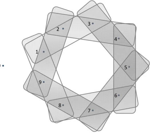
The cross-nested model that we estimated in the previous section is among the simplest of the new models that we can create using flexible generators. Many more models can be created using Proposition2. We shall now present an example where there is an ordering among products such that products that are nearer each other in the ordering are closer substitutes.
Products 1; :::; J are ordered in sequence. For simplicity, the ordering is cir-cular such that there are no endpoints. There is an outside option 0 with markets share q0. Define a flexible generator S by
S(j)(q) = ( q0; j = 0 q 0 j I11(j) I22(j) I33(j) ; j > 0; where I1(j) = qj 2+ qj 1+ qj; I2(j) = qj 1+ qj + qj+1; I3(j) = qj + qj+1+
qj+2 and parameters i are positive and sum to 1. This is a flexible generator by
Proposition 2. The structure is illustrated in Figure 3. There is a nest for any triple of neighboring products and each product is then in three nests. Then each product has its immediate neighbors as closest substitute and next neighbors as less close substitutes.
As before we simulated 1000 datasets from this model with 100 observations in each dataset. Variables zj and ~j are again respectively i.i.d. N (0; 1) and i.i.d.
0
1
2
3
4
9
8
7
6
5
Figure 3: Ordered structure of model in simulation example products and an out-side option
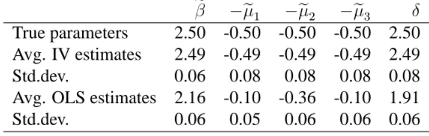
Table 2: Parameter estimates in simulation with ordered model
e e1 e2 e3
True parameters 2.50 -0.50 -0.50 -0.50 2.50 Avg. IV estimates 2.49 -0.49 -0.49 -0.49 2.49 Std.dev. 0.06 0.08 0.08 0.08 0.08 Avg. OLS estimates 2.16 -0.10 -0.36 -0.10 1.91 Std.dev. 0.06 0.05 0.06 0.06 0.06 ln qj = zj ~ ~1ln X j 2 i j qi ! ~2ln X j 1 i =j+1 qi ! ~3ln X j i j+2 qi ! + ln q0+ ~j;
using the same transformation of parameters as before. Note that we allow for three different values of ~i; although they all have the same true value ~i = 1= 0. As instruments we use 1; zj; P j 2 i jzi; P j 1 k =j+1zi; P j k j+2zi as well
as squares of these variables. F-statistics for the excluded instruments in the first-stage regression are again very high.
Estimation results are summarized in Table2. As before, the average of the IV estimates is close to the true value. The corresponding standard errors again seem small, considering that the datasets only have 100 observations. The average OLS estimates are again all more than two standard deviations from their true values, indicating again the necessity of accounting for endogeneity in the regression.
4
Discrete choice and generalized entropy
According to Theorem 2 there exists a generalized entropy that leads to a de-mand system that is not consistent with any ARUM. This section establishes that the class of demand systems (3) that can be created using generalized entropy includes all demands systems derived from ARUM. The class of generalized en-tropy demands is thus strictly larger than the class of ARUM demands.
We consider ARUM with utilities vj+"j; j 2 f1; :::; Jg, where v = (v1; :::; vJ)
is deterministic and " = ("1; :::; "J) is a vector of random utility residuals. The
joint distribution of " = ("1; :::; "J) is absolutely continuous with finite means and
independent of v. Suppose for simplicity that " is supported on all of RJ. Each consumer draws a realization of " and chooses the alternative = argmaxjfvj+ "jg
with the maximum utility, such that " is the residual of the maximum utility al-ternative. The expected maximum utility is denoted
G (v) = E (v + " ) : (12)
We denote the vector of choice probabilities as P (v) = (P1(v) ; :::; PJ(v)),
where Pj(v) = P ( = j). It is well known that P (v) = rG (v) (McFadden,
1981). All choice probabilities are everywhere positive since " has full support. The following lemma collects some properties of G and " .
Lemma 3 The function G is convex and finite everywhere. G has the homogeneity
property that G (v + c) = G (v) + c for any c 2 R, and G is twice continuously differentiable. Furthermore, G is given in terms of the expected residual of the maximum utility alternative by
G (v) = P (v) v + E (" jv) :
When the function G is convex and finite, it is also continuous and closed. Define
H (ev) =rv eG(v) : (13)
It follows directly from this definition that
rG (v) = H (e
v)
1 H (ev): (14)
In the case of the multinomial logit model, G (v) = lnPJj=1evj; H (ev) = ev,
such that (14) is the well known expression for the probabilities of that model. Lemma4is essentially the content of the appendix inBerry(1994). However, the proof in Berry relies on the existence of an outside option. The present proof
does not require an outside option to be present. The proof of Lemma 4 uses Lemma1, which allows it to be quite short.
Lemma 4 The function H defined by H (ev) = rv eG(v) is invertible.
The invertibility of H allows us to define
S (q) = H 1(q) : (15)
Let
G (q) = sup
v fq v
G (v)g (16)
be the convex conjugate of G (Rockafellar,1970, p. 104). Theorem4provides an explicit form for G (q), which underlies the findings that we present below. The function G (q) is finite only on the unit simplex , the set of probability vectors.
Theorem 4 The convex conjugate of the expected maximum utility G (v) is
G (q) = (
q ln S (q) ; q2 +1; q =2 :
Moreover, G (v) = supqfq v G (q)g and E (" jv) = G (q) when q = rG (v).
When " is an i.i.d. extreme value type 1 vector, then G (v) = ln (1 ev), while G (q) = q ln q is the Shannon entropy (Shannon, 1948). This shows that
G (q) is a generalization of entropy. We shall explore some properties of this
generalization.
The generalization of entropy G (q) is concave, since G is the convex
con-jugate of a convex function. It has maximum where 0 2 @G (q) or equivalently where @G (q) = fvjv = (c; :::; c) ; c 2 Rg. Hence it is maximal at the probabil-ity vector corresponding to vectors v that are constant across choice alternatives in the ARUM and do not affect the discrete choice. This is consistent with the interpretation of entropy as a measure of the expected surprise associated with a distribution.
may take any value, but it is necessarily positive when the random components have zero mean - this is a direct consequence of Jensen’s inequality.
Proposition 6 If E ("j) = 0 for all j in an ARUM, then the corresponding
gener-alized entropy is always non-negative: G (q) 0; q 2 .
We now turn to establishing the relation between ARUM and generalized en-tropy. The following two lemmas are used to show that a function S derived from an ARUM is a flexible generator as defined in Section2.
Lemma 5 The function S = H 1 is continuous, homogenous of degree 1, and satisfies Condition3.
We note by Lemmas 4 and 5 that an S derived from an ARUM via (15) is a flexible generator. The ARUM demand (14) is the same as the demand (3) resulting from maximization of utility (1). Then, by Theorem4, we have proved
Theorem 5 Let G be the convex conjugate of an ARUM surplus function G (v) =
E maxjfvj + "jg. Then G is a generalized entropy. The ARUM demand equals
the utility maximizing demand in Theorem1.
Section2.3provided an example of a generalized entropy that is not the convex conjugate of an ARUM surplus function.
4.1
Application to discrete choice data
We shall consider how to apply the generalized entropy model to microdata with observations of discrete choices. Such data are commonly available and provide the opportunity for incorporating individual specific information. The associated cost is that it is not possible to estimate microdata models merely by regression in the same way as with market level data. This section establishes an algorithm for computing the likelihood and applies this in an example to estimate a model using maximum likelihood. The ability to compute the likelihood is also useful with bayesian methods in combination with the Metropolis-Hastings algorithm.
We take as a starting point that individuals choose good j with probability qj
that probabilities sum to 1. If the generalized entropy in utility (1) is the convex conjugate of an ARUM surplus function, then q are simply the corresponding dis-crete choice probabilities. Generalized entropies that are not ARUM consistent may still correspond to nonadditive random utility models, i.e. models where util-ities are not just sums but more general functions of vj and "j (Matzkin, 2007).
Alternatively, individuals could be seen as making random choices with probabil-ities that are the result of utility maximization (Fudenberg et al.,2014).
We will consider estimation by maximum likelihood. This requires us to com-pute the likelihood q given v and we hence need a way to invert S that is feasible within a maximum likelihood routine. The following theorem indicates how the likelihood may computed by using an iterative process to solve a fixed point prob-lem. We use theKullback and Leibler(1951) distance function dr(q) = r ln rq
to evaluate the distance from the fixed point r to some q. This is a convex function with minimum at r with dr(r) = 0. Hence dr(q) will be larger the further q is
from r.
Theorem 6 Let S be the flexible generator defined in Proposition2and let r 2 satisfy v = ln S (r) + c for some c2 R. Then the mapping
w (q) = 8 > < > : qievi=S(i)(q) P j qjevj=S(j)(q) 9 > = > ; (17)
has r as unique fixed point and iteration of (17) from any starting point in converges to r.
If S has the form
S(j)(q) = q 0 j Y fg2Gjj2g;g6=fjgg q g g (18)
for some 0 > 0, then dr(w (q)) (1 0) dr(q).
Theorem6then shows that iteration of (17) will always converge to the fixed point. Intuitively, the numerator of (17) adjusts each qiin the direction that makes
Table 3: Maximum likelihood estimates in discrete choice simulation with cross-nested model 1 2 True parameters 0.500 0.500 0.200 0.500 Avg. estimates 0.498 0.498 0.208 0.495 Std.dev. 0.050 0.050 0.043 0.055
part of the theorem concerns the special case when the flexible generator is an average of the identity with something else. Beginning from q0 and iterating such that qn = w (qn 1) ; n 1 the theorem shows that dr(qn) (1 0)
n
dr(q0),
which means that the distance to the fixed point decreases exponentially
A question is now how well it is possible to recover parameters underlying utility from the observation of discrete choices. We have investigated this in a simulation experiment where we have simulated data from the cross-nested struc-ture of Section 3.1. We do not include the outside option as we have a situation in mind where we observe the choices of consumers who buy one of the varieties of some good under consideration. Utilities are specified as vj = x1j + x1jx2,
where x1j represents an alternative specific characteristic, while x2represents
in-dividual specific variation. We performed 100 replications with 1000 inin-dividuals in each, each individual selects 1 among the 9 alternatives in the model with prob-abilities q, where ln S (q) = v + c. The independent variables were generated as i.i.d. standard normal. The likelihood was computed using Theorem 6 and was maximized numerically.8 The results are summarized in Table3. As in the previ-ous simulations in this paper, we find that the true parameters are well recovered.
5
Concluding remarks
This paper has introduced the concepts of generalized entropy and flexible gener-ators and used them to derive a general family of demand systems. General rules for constructing demand systems have been provided along with some specific examples and it has been shown how these models may be estimated using either market share or individual level data.
We believe that generalized entropy models may be useful in a range of cir-cumstances. One example that we have mentioned is the demand for automobiles (e.g.Berry et al.,1995;Goldberg and Verboven,2001;Train and Winston,2007). The number of varieties of new cars is large and there are likely complex substi-tution patterns that may be accounted for using flexible generators. Another ap-plication area characterized by a large number of alternative "products" is spatial models, where flexible generators may be used to describe spatial correlations, for example in models of equilibrium sorting (Kuminoff et al., 2013). Yet an-other area where generalized entropy models may be useful are matching models (Salanié and Galichon, 2015), where the range of possible models could be ex-tended. It would also be of interest to develop generalized entropy models in the context of dynamic discrete choice models (Chiong et al., 2015). We hope that the family of demand systems provided here will stimulate future empirical work. The generalized entropy model extends to the case where the vector v is ran-dom with each consumer having some realization of v. Then demand conditional on v still has the form (3) and the expected demand is the expectation of (3). This is analogous to the mixed logit model (McFadden and Train, 2000). Moreover, both in the present case and in the mixed logit, the presence of the expectation implies that the explicit inversion in Theorem1does not carry through when v is random.
The nesting device we use to create flexible generators does not exhaust all possibilities. One possibility that we have not explored, for example, is to combine our nesting device with the idea that membership of a nest may be partial. There is thus scope for finding more flexible generators with properties that may be useful in specific circumstances.
Acknowledgements
We are grateful for comments from Yurii Nesterov, Bernard Salanié and Tatiana Babicheva as well from audiences at the conference on Advances in Discrete Choice Models in honor of Daniel McFadden at the University of Cergy-Pontoise, the Tinbergen Institute, the University of Copenhagen, Northwestern University, and Université de Montréal.
We have received financial support from the Danish Strategic Research Coun-cil, iCODE, University Paris-Saclay, and the ARN project (Elitisme).
References
Anderson, S. P., de Palma, A. and Thisse, J.-F. (1988) A Representative Consumer Theory of the Logit Model International Economic Review 29(3), 461.
Berry, S. (1994) Estimating discrete-choice models of market equilibrium The
RAND Journal of Economics 25(2), 242–262.
Berry, S. and Haile, P. A. (2014) Identification in Differentiated Products Markets Using Market Level Data Econometrica 82(5), 1749–1797.
Berry, S., Levinsohn, J. and Pakes, A. (1995) Automobile Prices in Market Equi-librium Econometrica 63(4), 841–890.
Birkhoff, G. (1946) Tres observaciones sobre el algebra lineal Universidad
Na-cional de Tucuman, Revista. Serie A 5, 147–151.
Chiong, K. X., Galichon, A. and Shum, M. (2015) Duality in dynamic dis-crete choice models Available at SSRN: http://ssrn.com/abstract=2700773 or
http://dx.doi.org/10.2139/ssrn.2700773 .
Fosgerau, M., McFadden, D. and Bierlaire, M. (2013) Choice probability gener-ating functions Journal of Choice Modelling 8, 1–18.
Fosgerau, M. and McFadden, D. L. (2012) A theory of the perturbed consumer with general budgets Working Paper 17953 National Bureau of Economic Re-search.
Fudenberg, D., Iijima, R. and Strzalecki, T. (2014) Stochastic Choice and Re-vealed Perturbed Utility Working Paper .
Goldberg, P. K. and Verboven, F. (2001) The Evolution of Price Dispersion in the European Car Market The Review of Economic Studies 68(4), 811–848.
Knittel, C. R. and Metaxoglou, K. (2014) Estimation of Random-Coefficient De-mand Models: Two Empiricists’ Perspective Review of Economics and
Kullback, S. and Leibler, R. A. (1951) On Information and Sufficiency The Annals
of Mathematical Statistics 22(1), 79–86.
Kuminoff, N. V., Smith, V. K. and Timmins, C. (2013) The New Economics of Equilibrium Sorting and Policy Evaluation Using Housing Markets Journal of
Economic Literature 51(4), 1007–62.
Mattsson, L.-G. and Weibull, J. W. (2002) Probabilistic choice and procedurally bounded rationality Games and Economic Behavior 41(1), 61–78.
Matzkin, R. L. (2007) Chapter 73 Nonparametric identification in J. J. H. a. E. E. Leamer (ed.), Handbook of Econometrics Vol. 6, Part B Elsevier pp. 5307– 5368.
McFadden, D. (1978) Modelling the choice of residential location in A. Karlquist, F. Snickars and J. W. Weibull (eds), Spatial Interaction Theory and Planning
Models North Holland Amsterdam pp. 75 –96.
McFadden, D. (1981) Econometric Models of Probabilistic Choice in C. Manski and D. McFadden (eds), Structural Analysis of Discrete Data with Econometric
Applications MIT Press Cambridge, MA, USA pp. 198–272.
McFadden, D. and Train, K. (2000) Mixed MNL Models for discrete response
Journal of Applied Econometrics 15, 447–470.
Melo, E. (2012) A representative consumer theorem for discrete choice models in networked markets Economics Letters 117(3), 862–865.
Mirsky, L. (1958) Proofs of two theorems on doubly stochastic matrices
Proceed-ings of the American Mathematical Society 9, 371–374.
Rockafellar, R. (1970) Convex analysis Princeton University Press Princeton, N.J.
Ruzhansky, M. and Sugimoto, M. (2014) On global inversion of homogeneous maps Bulletin of Mathematical Sciences pp. 1–6.
Salanié, B. and Galichon, A. (2015) Cupid’s Invisible Hand: Social Surplus and Identification in Matching Models Working Paper, Columbia University .
Shannon, C. E. (1948) A Mathematical Theory of Communication Bell System
Technical Journal 27(3), 379–423.
Train, K. E. and Winston, C. (2007) Vehicle choice behavior and the declining market share of u.s. automakers International Economic Review 48(4), 1469– 1496.
Verboven, F. (1996) The nested logit model and representative consumer theory
Appendixes
A
Proofs for Section
2
Proof of Theorem1. Form the Lagrangian
(q; ) = y + q v q ln S (q) + (1 1 q) :
The first-order conditions for (q1; :::; qJ) are
0 = @ @qk = vk ln S(k)(q) J X j=1 qj d ln S(j)(q) dqk ; resulting by Condition3in S (q) = ev > 0:
The homogeneity of S implies homogeneity of H = S 1and then
q = H ev = e ( + )H (ev) :
The constraint 1 q = 1 implies that e + = 1 H (ev) such that any solution to
the first-order conditions satisfies
q = H (e
v)
1 H (ev) (19)
and thus q is uniquely determined.
Existence of a solution is established as follows: Existence can fail only if the denominator in (19) is zero; but since the H(j)(ev) are non-negative, this can
only occur if H(j)(ev) = 0 for all j; this implies in turn by invertibility and
homogeneity of S that ev = 0, which is a contradiction. By Condition (2), the utility u (q) is concave, and hence the solution (19) to the first-order conditions is a global maximum.
so-lution to the utility maximization problem then it satisfies equation (3), which implies that
ln S (q) + ln (1 H (ev)) = v:
Conversely, if v = ln S (q) + c, then q solves (3).
Proof of Lemma1. This follows from Theorem 2.4 inRuzhansky and Sugimoto
(2014) upon noting that S may be extended to
f (x) = ( S (x) ; x2 (0; 1)J x; x2 RJ n (0; 1)J: Note that A RJ n (0; 1)J is closed , f is C1on RJ
nA with det Jf 6= 0 on RJnA,
f is continuous and injective on A, and RJ
nf (A) is simply connected. It is also
the case that f RJnA RJnf (A). Let fxng (0;1) J
with kxnk ! 1.
ThenkS (xn)k = kxnk S kxxnnk kxnk infq2 S (q)! 1. Since f satisfies
the conditions in theRuzhansky and Sugimoto(2014) theorem, S is invertible.
Proof of Lemma 2. (Averaging) Conditions 1-3 are easily verified. We shall verify that T is invertible using Lemma1. Since Tk(j)(q) qj, also S(j)(q) qj;
and then infqkS (q)k J 1 > 0, which is the first requirement in Lemma1.
The Jacobian of ln S is Jln S = K P k=1 kJln Tk:
Then Jln S is positive definite and hence its determinant is positive. The Jacobian
JS = diag S(1)(q) 1
; :::; S(J )(q) 1 J
ln S also has positive determinant, which
is the second requirement in Lemma1.
Proof of Proposition2. (General nesting) Condition1follows directly. Condi-tion2follows by noting that (q) is a linear combination of functions of the type
t ln t and that t! t ln t is strictly concave when t > 0. Finally, J X j=1 qj d ln S(j)(q) dqk = J X j=1 qj P g g1fj2gg1fk2gg@ ln (qg) @qk = X g2G g1fk2gg J X j=1 qj1fj2gg qg = 1
showing that Condition3holds as required. We have S(j)(q) = Y fg2Gjj2gg q g g Y fg2Gjj2gg q g j = qj:
The Jacobian of ln S has elements jk
X fg2Gjj2g;k2gg g 1 qg ;
such that it is symmetric and positive semidefinite. If it is positive definite, then by Lemma2S has an inverse and is a flexible generator.
Proof of Proposition3. (Invertible nesting) Observe that (6) may be written in matrix form as ln S (q) = M W ln M>q . Then
ln S (q) = v,
q = M> 1exp W 1M 1v :
Hence S has an inverse and it follows from Proposition 2 that S is a flexible generator.
Proof of Proposition 4. (Transformation) We shall verify Conditions1-4. Ob-serve that S defined by (8) is continuous and that for > 0,
S ( q) = exp ln + A>[ln (T (Aq))] + m = S (q) ;
since columns of A sum to 1. This verifies Condition1.
q 2 , T (Aq) + q m = Aq ln T (Aq) + q m = P i P j aijqj ! ln T(i)(Aq) + q m = P j qj P i aijln T(i)(Aq) + q m = q A>[ln (T (Aq))] + m = q ln S (q) :
Hence, T (Aq) + q m = q ln S (q). The transformation q ! T (Aq) q m
is concave on (Rockafellar,1970, Thm. 12.3) and then so is q ln S (q).
The next step is to verify Condition3. The condition holds by assumption for
T, and may be expressed as r T (q) = ln T (q) + 1. Now, with S(q) =
q A>[ln (T (Aq))] + m = (Aq)> [ln (T (Aq))] q m, we see that
r S(q) = A>( r T (Aq)) + m
= A>(ln T (Aq) + 1) + m = ln S (q) + 1
as required.
Finally, we shall verify the invertibility Condition 4by solving the equation
ln T (q) = v.
ln T (q) = A>[ln (S (Aq))] + m = v , q = A 1H exph A> 1(v m)i :
Thus, T is invertible. This completes the proof.
Proof of Proposition5. (Nesting) Consider the function S defined by (9). Con-dition1is clearly satisfied. Generalized entropy corresponding to S is
(q) = q1 ln T1
q1
1 q1 1 q
1; q2 ln T
which is concave and then Condition2is satisfied. For q = (q1; q2) = (q 1; :::; qJ1+J2 1), and with r = q1 1 q1, we have J1+JP2 1 j=1 qj @ ln S(j)(q) @qk = 1fk J1g J1 P j=1 qj1 @ ln T1(j) 1 qq11 @qk + 1 q1 @ ln T (1) 2 (1 q1; q2) @qk + JP2 1 j=2 qJ1+j @ ln T2(j)(1 q1; q2) @qk = 1fk J1g 1 q1 J1 P j=1 rj J1 P i=1 @ ln T1(j)(r) @ri @ri @qk + 1 = 1fk J1g 1 q1 J1 P j=1 " rj J1 P i=1 @ ln T1(j)(r) @ri 1fi=kg 1 1 q1 ri 1 q1 # + 1 = 1fk J1g 1 q1 J1 P i=1 " 1fi=kg 1 1 q1 ri 1 q1 J1 P j=1 rj @ ln T1(j)(r) @ri # + 1 = 1fk J1g 1 q 1 PJ1 i=1 1fi=kg 1 1 q1 ri 1 q1 + 1 = 1; which is Condition3.
Finally, to show that S is invertible, consider the equation ln S (q1; q2) =
(v1; v2). Let q1 = T 1 1 ev 1 , r = 1 q1, and let (rs; q2) = T2 1 r; ev2 . Then for j J1 ln S(j) sq1; q2 = ln T1(j) q 1 r + ln T (1) 2 rs; q 2 = ln T1(j) q1 ln r + ln T2(1) rs; q2 = v1j ln r + ln T2(1) rs; q2 = vj1: For j > J1 we have ln S(j) sq1; q2 = ln T(j J1) 2 rs; q 2 = v2 j:
Then
S 1 ev1; ev2 = sq1; q2
= sT1 1 ev1 ; q2
and Condition4is satisfied. Thus, S is a flexible generator.
B
Proofs for Section
4
Proof of Lemma3. Fosgerau et al.(2013) establishes convexity and finiteness of G as well as the homogeneity property and the existence of all mixed partial derivatives up to order J . This also implies that all second order mixed partial derivatives are continuous, since J 3.
The existence of derivatives Giiis established from the homogeneity property
that Gj(v + c) = Gj(v) ; j = 1; ; ; :; J . Consider G11at no loss of generality and
observe that G1(v1+ c; v2; :::; vJ) G1(v1; v2; :::; vJ) c = G1(v1; v2 c; :::; vJ c) G1(v1; v2; :::; vJ) c ! c!0+ P j6=1 G1j(v) = G11(v) ;
which means that G11 exists. Furthermore, G1j; j > 1 are continuous and hence
so is G11:
Let be the index of the chosen alternative. The last statement of the lemma follows using the law of iterated expectations since
G (v) = P j E max j fvj + "jg j = j; v Pj(v) = P j (vj + E (" j = j; v)) Pj(v) = P (v) v + E (" jv) :
Proof of Lemma 4. We shall make use of Lemma 1 applied to H. The Jaco-bian of v ! H (ev) is eG(v)G
i(v) Gj(v) + eG(v)Gij(v) . The first matrix
is positive definite since all choice probabilities are positive, the second matrix is positive semidefinite due to the convexity of G, hence this matrix is every-where positive definite and then the Jacobian determinant of v ! H (ev) never
vanishes. This implies in turn that the Jacobian determinant of the composition
y ! ln y ! H (y) never vanishes. It remains to show that infy2 kH (y)k > 0.
But y 2 implies that
kH (y)k = eG(ln y)krG (ln y)k eE maxjfln yj+"jgJ 1=2 emaxjfln yj+E"jgJ 1=2 = max j yje E"j J 1=2 y1eE"1; :::; yJeE"J J 1 J P j=1 e 2E"j ! 1 J 1 > 0;
where we first used thatrG is on the unit simplex, second that the max operation is convex, third that the sup-norm bounds the euclidean norm, and fourth that the minimum of y1eE"1; :::; yJeE"J on the unit simplex is attained at yj =
e 2E"j J P k=1 e 2E"k 1 ; j = 1; :::; J .
Proof of Theorem4. We first evaluate G (q). If 1 q6= 1, then
q (v + ) G (v + ) = q v G (v) + (1 q 1) ;
which can be made arbitrarily large by changing and hence G (q) = 1. Next consider q with some qj < 0. G (v) decreases towards a lower bound denoted
G ( 1; v j) as vj ! 1. Then q v G (v) increases towards +1 and hence
G is +1 outside the unit simplex .
For q 2 , we solve the maximization problem (16) noting that we may fix
conditions 0 = qj Gj(v) , which lead to = 0. Then q = rvG (v), qeG(v) = rv eG(v) = H (ev), S (q) eG(v) = ev , ln S (q) + G (v) = v ) q ln S (q) + G (v) = q v:
Inserting this into (16) leads to the desired result.
G is convex and closed and hence G is the convex conjugate of G ( Rock-afellar, 1970, Thm. 12.2), this is the next assertion of the theorem. Finally, for
q = rG (v), a fundamental result of convex analysis (Rockafellar, 1970, Thm. 23.5) states that G (v) + G (q) = v q, which may be combined with (12) to yield the final statement of the theorem.
Proof of Proposition6. Note that the maximum is a convex function, such that Jensen’s inequality applies. Then, for q =rG (v),
G (q) = E max
j (vj+ "j) v q
max
j E (vj+ "j) v q 0:
Proof of Lemma 5. Continuity of S follows from continuity of the partial derivatives of G, which is immediate from the definition.
Homogeneity of S is equivalent to homogeneity of H. Using the homogeneity property of G,
S 1( ev) = rv eG(v+ln ) = rv eG(v) = S 1(ev) ;
which shows that H and hence S are homogenous of degree 1. The requirement thatXJ
j=1qj
d ln S(j)(q)
dqk = on relint ( ) may be expressed
in matrix notation in terms of the Jacobian Jln S(q1; :::; qJ) of ln S as (q1; :::; qJ)
With v = ln S (q) and noting that (ln S) 1(v) = H (ev), the requirement is equivalent to (q1; :::; qJ) = (q1; :::; qJ) Jln S(q) J(ln S) 1(v) = (1; :::; 1) JH(ev)(v) : Now, (1; :::; 1) JH(ev)(v) = (1; :::; 1) eG(v)Gj(v) Gk(v) + eG(v)Gjk(v) 1fj=kg = (q1; :::; qJ)
as required. We have used first that
(q1; :::; qJ) = H (ev) ;
and second that (1; :::; 1) fGjk(v)g = 0, where the latter assertion follows since
1 = PJj=1Gj(v).
Proof of Theorem6. Note thatPg grg =PjPfgjj2gg grj = 1. We will first
show existence and uniqueness of a fixed point. Note that for r 2 :
w (r) = 8 > < > : rievi=S(i)(r) P j rjevj=S(j)(r) 9 > = > ;= 8 > < > : riS(i)(r) =S(i)(r) P j rjS(j)(r) =S(j)(r) 9 > = > ;= r;
which shows that r is a fixed point. If q 2 is a fixed point, potentially different from r, then qi = qi evi=S(i)(q) e c, where ec =
P
jqje
vj=S(j)(q), and then
v = ln S (r) + c. The invertibility of S implies that q = r and then the fixed point
is unique.
We then need to show that iterations with (17) from any starting point in converges to the fixed point. Define for convenience
j = S(j)(r) S(j)(q) = Q fgjj2gg rg qg g ; wj(q) = qievi=S(i)(q) P j qjevj=S(j)(q) :
Using that v = ln S (r) + c with c2 R we may rewrite (17) as wj(q) = qjevj=S(j)(q) P i qievi=S(i)(q) = qjS (j)(r) S(j)(q) P i qiS (i)(r) S(i)(q) = qj j q :
We will show that dr(w (q)) dr(q), with strict inequality when q 6= r. This
will mean that w (q) is closer to r than q. Evaluating dr(w (q)) leads to
dr(w (q)) = r ln r w (q) = r ln 0 @n r qj j q o 1 A = dr(q) + ln (q ) r ln = dr(q) + ln P j qj Q fgjj2gg rg qg g! P j rjln Q fgjj2gg rg qg g :
We thus need to bound the last two terms. Observe first that
ln P j qj Q fgjj2gg rg qg g! = ln P j qjexp P fgjj2gg gln rg qg ! ln P j P fgjj2gg qj g rg qg ! = ln P g P fjjj2gg qj g rg qg ! = ln P g g rg = 0;
with strict inequality unless rg = qgfor all g. Equality would imply S (r) = S (q),
We also need to bound P j rjln Q fgjj2gg rg qg g = P j P fgjj2gg rj gln rg qg = P g g rgln rg qg = P g g rgln grg gqg 0;
where the last inequality follows since the term is a Kullback-Leibler distance. We conclude that dr(w (q)) dr(q) and that the inequality is strict unless r = q.
Now consider a sequencefqng constructed by iterating (17). Then dr(qn) is
weakly decreasing and hence dr(qn) ! for some 0. If > 0, then a
convergent subsequence can be extracted fromfqn
g with limit point ^q satisfying dr(^q) = by continuity of w. Now dr(w (^q)) < , while there are points from the
sequencefqng arbitrarily close to ^q with dr(qn) > . This contradicts continuity
of w and we conclude that = 0 and hence that qn ! r.
If furthermore S has the form (18), then we can improve the bound on dr(w (q)):
dr(w (q)) dr(q) = ln P j qj Q fgjj2gg rg qg g! P j rjln Q fgjj2gg rg qg g P j rjln " rj qj 0 Q fgjj2g;fjg6=gg rg qg g# = 0r ln r q P j rj P fgjj2g;fjg6=gg gln rg qg 0dr(q) ;
Glossary
p Price vector
P Probability vector
q; r Consumption vector of the differentiated good, probability vector
S Flexible generator
G Expected maximum utility
G Convex conjugate of G
H Inverse of S
a Vector of intrinsic utilities of the differentiated good Generalized entropy v (a p) ; Utility parameters u Utility Nesting parameter Unit simplex k k Euclidian norm
Marginal utility of income Index of chosen alternative