HAL Id: hal-00630200
https://hal.archives-ouvertes.fr/hal-00630200
Submitted on 7 Oct 2011HAL is a multi-disciplinary open access
archive for the deposit and dissemination of sci-entific research documents, whether they are pub-lished or not. The documents may come from teaching and research institutions in France or abroad, or from public or private research centers.
L’archive ouverte pluridisciplinaire HAL, est destinée au dépôt et à la diffusion de documents scientifiques de niveau recherche, publiés ou non, émanant des établissements d’enseignement et de recherche français ou étrangers, des laboratoires publics ou privés.
Demographic structure and capital accumulation
Hippolyte d’Albis
To cite this version:
Hippolyte d’Albis. Demographic structure and capital accumulation. Journal of Economic Theory, Elsevier, 2007, 132 (1), pp.411-434. �hal-00630200�
Demographic structure and capital
accumulation
Hippolyte d’Albis
GREMAQ, University of Toulouse I, 21 allée de Brienne, 31000 Toulouse, France
Abstract
This paper develops an overlapping generations model to analyze the conse-quences of demographic structure changes induced by an exogenous shift in the birth rate. We …rst show that a …nite growth rate of the population that maximizes long-run capital per capita exists. Then, we examine the theoretical properties of this growth rate by showing that: (i) it corresponds to the demographic struc-ture such that the average ages of capital holders and workers are equal; (ii) it is associated to an e¢ cient steady state; (iii) it increases with compulsory transfers from younger to older generations. Finally, we explain why standard overlapping generations models do not exhibit such a growth rate.
JEL Classi…cation: D91; E13; J10
Key words: Continuous-time overlapping-generations models; Population aging
1 Introduction
Overlapping generations (OLG) models are the neoclassical literature’s com-mon tool for analyzing the economic consequences of demographic structure changes. In this paper, we focus on the impact of exogenous shifts in the birth rate on long-run capital accumulation. This relationship is crucial for ana-lyzing the consequences of population aging on most macro-variables1, such
as growth, assets prices and unemployment. An increase in the population growth rate simultaneously induces a reduction in capital per worker and an increase in savings; the problem is to …nd out which one has the strongest e¤ect. Standard OLG models with production in discrete or continuous time developed by Diamond [13] and Blanchard [4], respectively, can be used to
0 E-mail address: [email protected].
show that a birth-rate increase reduces long-run capital per capita. The eco-nomic intuition given to this result relies on the absence of intergenerational altruism: the size of future generations does not directly in‡uence the saving choices of current generations. The reduction in aggregate consumption that follows a birth rate increase is therefore insu¢ cient for compensating the cap-ital dilution e¤ect. Following Weil [36], the birth rate measures the degree of disconnection between generations, and newborn individuals are interpreted as “unloved children” or immigrants.
Empirical studies, however, do not show that demographic structure changes have a signi…cant impact of on capital accumulation or, more precisely, on its marginal productivity. In a recent paper, Poterba [30] analyzes the historical relationship between population structure and assets return, including the interest rate. Using time series from the United States, Canada and the United Kingdom for the last seventy years. Poterba …nds no robust evidence of any impact of demographic variables on assets prices.
At a …rst glance, these empirical …ndings seem to invalidate the OLG models while validating the Ramsey framework. In this framework2, where the
popu-lation is composed of one unique, altruistic family, the demographic variables have no impact at the balanced equilibrium. That is because the optimal response to a birth-rate increase is to reduce consumption in order to keep capital per capita constant. However, in this paper, we argue that Poterba’s results can be reproduced in an OLG model. We build a continuous time OLG model of individuals with …nite life-spans to show there exists a …nite population growth rate, or equivalently an age structure of the population, that maximizes capital per capita. The existence of this capital maximizer implies that (i) the sign of the impact of demographic growth on capital per capita is ambiguous; (ii) the two di¤erent demographic structures could be associated to the same capital per capita; (iii) and the demographic structure changes have a little impact on capital per capita when these structures are at the neighborhood of the one that maximizes capital per capita. Hence, we conjecture that the demographic structures of developed countries have re-mained close to the structure which maximizes capital per capita. Of course an estimation is required to prove this statement, which is not within the scope of this paper. Instead, we focus on the theoretical characterization of the demographic growth rate that maximizes steady-state capital per capita.
Our argument hinges on the simple but crucial assumption of a population composed of non-altruistic individuals who accumulate assets following a life-cycle behavior. This is standard in neoclassical literature, but is barely im-plemented in general equilibrium models, because of the technical di¢ culties that arise in the aggregation procedure. Thus, the two-period lifetime model
by Diamond [13] and the continuous time models by Blanchard [4] and Weil [36], which avoid these di¢ culties, are therefore extensively used in the lit-erature. We show, however, that the assumptions that keep these models tractable, are responsible for the monotonic relationship they exhibit between population growth and capital per capita.
We argue that it is possible to develop an analytically tractable model that reproduces the stylized fact highlighted by Poterba [30]. We build a continuous time OLG model of individuals with …nite life-spans based on the pioneering works of Tobin [33] and of Cass and Yaari [10]3. We assume a general pat-tern of individual mortality, which includes such cases as the certain lifetime, the Blanchard’s Poisson process and the Weil’s in…nitely-lived families. This formalization makes the comparative discussion straightforward. Aggregation is made following Lotka’s [27] assumption of a stable population structure as well as assumptions of perfect …nancial and insurance markets.
We then derive the following results. First, we give su¢ cient conditions for the existence and uniqueness of a steady-state path. These conditions, which are easy to interpret and compare with the existing OLG literature. We then perform a static comparative analysis and show that a …nite population growth rate that maximizes capital per capita exists. This result crucially depends on the …niteness of individual life-span. Moreover, the considered growth rate corresponds to the demographic structure, such that the average age of capital holders weighted by their wealth equals the average age of the workers weighted by their earnings. We demonstrate this result using the property of stable populations to exhibit easily averaged ages associated to individual variables4. Thus, in the steady-state equilibrium, the impact of demographic growth on capital per capita is positive if the average age of capital holders is lower than the average age of workers. By construction, this case cannot exist in the Diamond [13] and Blanchard [4] models.
Before introducing the model, we want to emphasize that our analysis is pos-itive. Indeed, our intention is di¤erent from the issue raised by Samuelson [31] on the optimal population growth rate. This growth rate is the one that maximizes welfare when the equilibrium is golden-rule. Instead, we make a static comparative analysis when the equilibrium is balanced. Nevertheless, we show that the equilibrium associated to the demographic growth rate that maximizes capital per capita, is e¢ cient. Moreover, we complete the analy-sis by introducing compulsory transfers between generations and show that transfers from younger to older generations increase the demographic growth
3 Further developments have been made recentely by Burke [8], Malinvaud [28], Bommier and Lee [5] and Demichelis and Polemarchakis [12].
4 These were …rst introduced in economic models by Arthur and McNicoll [2] and Lee [26].
rate that maximizes capital per capita.
The basic framework of the model is presented in Section 2 and the analysis of the e¤ect of a shift in the demographic growth rate on the steady-state capital per capita is made in Section 3. A general discussion of the results is proposed in Section 4. Section 5 concludes and the Appendix presents all the proofs of the propositions.
2 The model
This section presents an aggregation of individual consumption behavior un-der an uncertain lifetime in an overlapping generations model of neoclassical growth. It presents the steady state of such an economy and derives su¢ cient conditions for its existence and uniqueness. Time is continuous, and all the variables that depend on time are assumed to be continuous and di¤erentiable.
2.1 Individual behavior
We closely follow Yaari [37]5. Individuals are uncertain about the length
of their life. Let ( ) > 0 denote the probability density function of the random variable with support [0; ], where is the …nite maximum possible lifetime. Individuals also exhibit a pure discount factor ( ) that satis…es : (0; ] ! (0; 1) and (0) = 1; hence, the pure discount rate, denoted ( ) 0( ) = ( ) which may vary with age and might even be negative. Individuals only derive satisfaction from their consumption, denoted c ( ) 0and have no bequest motives. Instantaneous utility is isoelastic with an elasticity of intertemporal substitution 2 (0; 1]. Hence, expected utility at birth of any individual is:
Z 0 ( ) 0 @Z 0 (z)c (z) 1 1= 1 1 1= dz 1 Ad (1)
During a lifetime, the labor supply is …xed and, w ( ) > 0; a given stream of labor income is received. There is a single asset and individuals have access to competitive capital and complete insurance markets. Individuals hence hold their entire wealth a ( ) in the form of actuarial notes that makes an insurance company their legatee. Since the notes are assumed actuarially fair, they
5 Our problem is less general, however, since we are considering a speci…c instan-tanous utility function, namely a CRRA with 2 (0; 1]. Relaxing this assumption drastically complicates the proof of the existence of an aggregate equilibrium.
yield the regular risk-free interest rate, r > 0; plus the hazard rate of death and are therefore the most lucrative asset if the individual wealth is positive. Moreover, the uncertainty about life-span makes the subscription to these notes the only way to borrow. Let p ( ) =R (z) dzdenote the probability at birth that an individual will be alive at age . Hence, (zj ) = (z) =p ( ) is the conditional probability density evaluated at age z, given that the individual is alive at age , and ( j ) is the hazard rate of death at age . The hazard rate of death is supposed to be non-decreasing with respect to age:
0( j ) 0. The individual budget constraint hence writes:
a0( ) = [r + ( j )] a ( ) + w ( ) c ( ) (2) Individuals are born with no …nancial assets and face a terminal condition that forbids Ponzi games. The two following conditions therefore complete the individual program:
a (0) = 0 (3)
a ( ) 0 (4)
We, moreover, assume that ( ), ( ), w ( ) and a ( ) are of class C2 on
[0; ] and that c ( ) is of call C1 on [0; ]. For simplicity’s sake, we de…ne
G (:) and H (:) such that:
G (x) Z 0 p ( ) w ( ) exp ( x ) d (5) H (x) Z 0 p ( ) [ ( )] exp ( x ) d (6)
which are both positive and decreasing. Note thatR0 p ( ) exp ( r ) d rep-resents the expected discounted value of a constant ‡ow of one unit of output; this value is weighted with the income distribution in G (r) and with the pref-erence parameters in H (r).
Given prices r and w, each individual chooses fc ( )g that maximizes (1) subject to (2), (3) and (4). The optimal behavior is now described by the following proposition:
Proposition 1 There exists a unique solution to the individual problem. For 2 [0; ], the optimal consumption pro…le satis…es:
c ( ) = G (r)
while the optimal wealth satis…es:
a ( ) =
Z p (z)
p ( )exp ( r (z )) [c (z) w (z)] dz (8) with a ( ) = 0.
The individual behavior described by equation (7) is the standard neoclassical one. Note that G (r) =H ((1 ) r)represents the product of the expected dis-counted ‡ow of earnings at birth and the marginal propensity to consume out of total individual wealth at birth, i.e. the initial consumption c (0). Deriving equation (7) with respect to yields:
c0( ) = [r ( )] c ( ) (9) Perfect annuity markets imply that the optimal consumption growth rate only depends on the di¤erence between the interest rate and the pure discount rate. Since the latter varies with age, individual consumption may then decrease during the life-span. Moreover, it may also be a concave function of age if the pure rate of discount su¢ ciently increases with age.
Concerning the optimal asset accumulation, its pro…le is characterized in the following proposition:
Proposition 2 For 2 [0; ], the optimal wealth is positive and hump-shaped if: [r ( )] > 0( j ) ( j ) and 0( j ) r + ( j ) > w0( ) w ( ) (10)
A borrowing period during the life-cycle is a possible output of the individual problem. However, under rather plausible assumptions, proposition 2 rules out this possibility. It is indeed su¢ cient to have a consumption growth rate greater than the hazard rate of death’s growth rate and a bounded income growth rate. Remark that the hazard rate of death is usually assumed by demographers to follow a Gompetz’ law such that ( j ) = exp (x ) with x > 0. Alternatively, if the individual consumption is decreasing during the life-span, the optimal wealth may not be hump-shaped. Finally, note that condition (10) remains to be check at the equilibrium since it involves the interest rate that is to be an endogenous variable.
Remark 1. Our rather general speci…cations ease the comparison with OLG models developed by Blanchard [4] and Weil [36]. Blanchard assumes that an individual lifetime follows a Poisson process and that the pure discount rate and the wage stream are constants. With our notation, =1, ( j ) = p; ( ) = , and w ( ) = w with p; ; w > 0. Thus, G (x) = w= (x + p) and H (x) = 1= (x + p + ). It is moreover necessary to replace condition (4) by
the No-Ponzi-Game condition: lim
!+1exp ( (r + p) ) a ( ) 0. Weil
inter-prets the individual as an in…nitely lived family, an assumption that can be obtained by setting p = 0. Replacing in equation (7), the individual consump-tion behavior becomes for all 0:
c ( ) = w[(1 ) r + p + ]
(r + p) exp ( (r ) ) (11) Simple manipulations of equation (11) yields the individual asset accumula-tion:
a ( ) = w
(r + p)[exp ( (r ) ) 1] for 0 (12) In Blanchard and Weil models, the consumption and asset accumulation pro-…les are hence a monotonic function of age.
2.2 Aggregation and competitive equilibrium
The demographic structure is based on Lotka’s [27] stable population theory. Each individual belongs to a large cohort of identical individuals. Therefore even though each individual’s life-span is stochastic, there is no aggregate uncertainty. The law of large numbers is supposed to apply6, and thus, the size of each cohort is decreasing at rate ( j ). Then, at time t, the size of the age- cohort is N (t ) p ( ) where > 0 is the birth rate and N (t ) is the size of the population at time t . Since a new cohort is born at each instant, N (t) satis…es:
N (t) =
Z
0
N (t ) p ( ) d (13)
Lotka demonstrates that the demographic structure (i.e. the relative size of each cohort in the population) reaches a steady state when the birth and death rates have been constant over a su¢ ciently long period of time. The stationary distribution, characterized by the demographic growth rate n, is obtained by replacing N (t) = N (0) exp (nt) in (13) and then solving:
Z
0
p ( ) exp ( n ) d = 1 (14)
The unique real solution of equality (14) de…nes7 the population growth rate n whose sign depends on the di¤erence between the birth rate and the inverse of the life expectancy at birth. Formally, n 0if and only if 1=R0 p ( ) d .
6 See the discussion in Judd [21] and Feldman and Gilles [16].
7 The left hand side of (14) is a positive, decreasing function of n, whose limits are respectively +1 and 0 when n goes to 1 and +1.
Note that the relative size of each cohort in the population, p ( ) exp ( n ), is then time independent, which is why the population is said to be stable.
Aggregate wage per capita, denoted as w, satis…es:
w
Z
0
p ( ) exp ( n ) w ( ) d (15)
while consumption per capita, denoted as c, satis…es:
c
Z
0
p ( ) exp ( n ) c ( ) d (16)
Hence, replace equation (7) in (16) and replace using (5) and (15), to obtain:
c = wG (r) G (n)
H (n r)
H ((1 ) r) (17) Moreover, when the individuals consumption pro…le is optimal, aggregate …-nancial wealth per capita, denoted as a, satis…es8:
a = c w
r n (18)
There is a unique material good, whose price is normalized to 1. It can be used for consumption or for adding to the capital stock. This good is produced by many competitive …rms whose aggregate activity is described by a constant return-to-scale production function with labor and capital as inputs. Let k be the capital per capita, 0 be the depreciation rate and f (:) be the production function in intensive form. Assume that f : [0; 1) ! [0; 1); that f0(k) > 0and f00(k) < 0for all k > 0, and that lim
k!0f
0(k) =1. Factor prices
equal marginal products; hence w = f (k) kf0(k) and r = f0(k) .
As in Diamond [13] and Blanchard [4], the equilibrium condition is obtained by identifying asset holdings with capital stock: a = k. The analysis of steady-state equilibrium turns out to be a …xed-point problem, k = (k), where func-tion is obtained by …rst replacing equation (17) in (18) and then replacing factor prices such that:
(k) f (k) kf 0(k) f0(k) (n + ) " G (f0(k) ) G (n) H (n (f0(k) )) H ((1 ) (f0(k) )) 1 # (19)
Let us introduce s (k) kf0(k) =f (k), the share of capital in output and " (k) f0(k) [1 s (k)] = [kf00(k)], the elasticity of substitution between
cap-ital and labor. The concavity of f implies that s 2 (0; 1) and " > 0 for all k > 0.
Proposition 3 There exists ^k > 0 such that ^k = ^k if lim k!0[ kf 00(k)] > 1 (20) ^ k is unique if s (k) " (k) and d dk s (k) " (k) ! 0 (21)
Proposition 3 gives existence and uniqueness conditions for a non-trivial equi-librium. Technically, condition (20) implies lim
k!0 (k) = +1 and conditions
(21) ensure 0 k < 1. Let us now turn to the interpretation.^
Our existence condition (20) is close to the condition proposed by Bommier and Lee [5] who extend to a continuous-time framework the …ndings of Konishi and Perera-Tallo [23] for the Diamond model [13]. Their condition, named the “non-vanishing labor share”, has the advantage of relying only on the production function. Formally it can be written as:
lim
k!0s (k)2 [0; 1) (22)
However, (22) is more restrictive than (20). To demonstrate that point, let us observe that lim k!0 " 1 s (k) s (k) f 0(k) # lim k!0[ kf 00(k)] (23)
Let us now recall the Inada condition on f0(k)and conclude that (22) implies
lim
k!0[ kf
00(k)] = +1.
In condition (20), the key elements are the maximum possible lifetime and the elasticity of inter-temporal substitution. Strong income e¤ects yielded by a small , may hence be compensated by a longer lifespan. Moreover, in Blanchard [4] and Weil’s [36] models, where =1, a competitive equilibrium always exists.
Multiple equilibria may occur in such a framework: see notably Kehoe [22] for production economies and Ghiglino and Tvede [18] for economies with heterogeneous endowments. Further restrictions on the production function are hence needed to exclude this possibility. Our conditions (21) state that inputs should be rather substitutable, especially if capital per capita is low at equilibrium. These conditions are notably satis…ed by production functions with a constant elasticity of substitution that is greater than one (" 1); that is the functions that verify the Inada condition for k = 0. Let us also note that relaxing the assumption of 2 (0; 1] may produce multiple equilibria.
Remark 2. The complete analysis of the inter-temporal equilibrium is be-yond the scope of this paper. Note nevertheless, that recent contributions have pointed out the importance of the initial condition of the economy on the existence of the equilibrium. Burke [8] notably extend to continuous time the result that the equilibrium may fail to exist if time has a …nite start-ing point (See Geanakoplos and Polemarchakis [14]). As a consequence, the particular solution that is given by the steady-state equilibrium may also fail to exist. Moreover, the dynamics of the equilibrium path is not necessar-ily monotoneous: in a pure exchange economy, Demichelis and Polemarchakis [12] show the existence of exponnentially decreasing ‡uctuations along the transition while Ghiglino and Tvede [19] show that a cycle may exist.
A graphical illustration. We propose a graphical example of the equilib-rium in the (k; c) space when conditions (20) and (21) are respected. Note …rst that equation (18) may be written as c = (r n) a + w; at the equilibrium, this de…nes c1(:) such that:
c1(k) = f (k) (n + ) k (24)
The c1(k)line represents the resource constraint of the economy. If n + > 0,
c1(k) is hump-shaped with golden-rule consumption that occurs at the point
where c1(k) reaches its maximum. Then, we use the de…nition of the wages
given above and replace it in (17); at the equilibrium, this de…nes c2(:) such
that:
c2(k) =
k [f0(k) (n + )]
1 G(fG(n)0(k) )H((1H(n )(f(f0(k)0(k) )))) (25)
The c2(k) line stands for the aggregation of individual consumption decisions
for each level of capital. Here, for example, …gure 1 represents9 the situation
where n + > 0, f (0) = 0 and there is dynamic e¢ ciency.
6 c - k c1 c2 pppppppp pppppppp pppppppp pppppppp pppppppp pppppppp pppppppp pppppppp ppp ^ k Figure 1
This …gure is the extension, for any stationary demographic structure, of the one presented in Blanchard [4].
3 Demographic growth and capital per capita
This section analyses the impact of a shift in the population growth rate on the steady-state capital per capita and shows that a …nite growth rate that maximizes capital per capita exists. It then characterizes this capital maximizer.
3.1 Main results
It is useful to de…ne x, the average age calculated cross-sectionally such that:
x R 0 p ( ) exp ( n ) x ( ) d R 0 p ( ) exp ( n ) x ( ) d (26)
where x ( ) is a relevant characteristic. In the case x ( ) = 1; 1 is the
standard de…nition of the average age of the population. If x ( ) = w ( ) ;
w is the average age of workers weighted by their earnings and equivalently,
if x ( ) = a ( ) ; a is the average age of capital holders weighted by their
wealth.
We now implicitly consider that the change in the demographic growth is induced by a change in the birth rate. It is, however, not worth represent-ing changes in the birth rate since its long-run relationship with demographic
growth is monotonously increasing. Indeed, implicit di¤erentiation of condi-tion (14) yields: dn d = 1 1 > 0 (27)
Hence, a static comparative of demographic growth on steady-state capital per capita yields the following result:
Proposition 4 The impact of an increase in population growth on capital per capita depends on the di¤erence between the average age of capital holders and the average age of workers; one indeed has:
d^k dn =
^ k
1 0 ^k [ a w] (28)
Proposition 4 states that an increase in population growth does not neces-sarily reduce the steady-state capital per capita but depends on income and population distributions. Observe moreover that ais an endogenous variable
while w is exogenous. The interpretation of this result will be given after the
next proposition.
Proposition 5 There exists a …nite value of the population growth rate, de-noted as n , that maximizes steady-state capital per capita.
Propositions 4 and 5 show that the relationship between the population growth rate and steady-state capital per capita is non monotonic and that capital per capita reaches a maximum when the average age of capital holders equals the average age of workers. The intuition of this result can be obtained by comparing the impact of demographic growth on the age structure of the working population and the pattern of individual assets. Let us …rst observe that the average age of the workers is decreasing with n; at the limit, it equals 0 for n = +1 and for n = 1. Next, let us recall that the optimal asset accumulation pattern during lifetime is such that a (0) = a ( ) = 0. Therefore, when n goes to plus or minus in…nity, (i.e. when 1 goes to 0 or ) the capital
accumulated in the economy is very low. Conversely, the steady-state capital per capita is maximal when the distribution of population concentrates a large mass of individuals around the maximum wealth in the life-cycle accumulation pro…le. Remark that Proposition 5 does not rule out multiples n . Observe nevertheless, that if n is unique, the relationship between n and k is hump-shaped.
Remark 3.An n-maximizer has also been recently presented in Boucekkine, de la Croix and Licandro [6]. In an endogenous growth model with schooling and retirement choices, they …nd a hump-shaped relationship between the population growth rate and the per-capita growth rate of human capital. Their
result is based on a functional but realistic survival law and an instantaneous utility that is linear with respect to consumption. There is no capital in their model, but the existence of an n-maximizer relies on the same reasoning: the vintage structure of human capital.
3.2 Optimality
The population growth rate that maximizes capital per capita is not optimal since it does not maximize individual welfare or aggregate consumption; it can be only stated that the equilibrium to which it is associated with is e¢ cient. To see that point, let us …rst consider the following proposition:
Proposition 6 Let k be such that k = 0 and such that f0 k = + .
Then,
n < (29)
Proposition 6 introduces , the lower bound on the interest rate, associated to k, the maximal value for capital per capita at equilibrium. This bound corresponds to the interest rate above which outstanding debt in the economy outweighs positive assets. If the individual pure discount rate is constant, such that ( ) = , then = . Otherwise, depends on the model parameters, including demographic ones. Thus, proposition 5 states that the population growth rate that maximizes capital per capita is lower than the lower bound on the interest rate. This result is quite intuitive if the individual consumption pro…le is supposed to be increasing: then, the age at which individuals have a maximal wealth takes place during the second half of their lives. Therefore, capital per capita is maximized by a demographic structure with a relatively high average population age, which means a rather low population growth rate.
Corollary 1. At the steady-state equilibrium associated with n , there is under-accumulation of capital.
The de…nition of , given in proposition 6, implies that any steady-state ^k sat-is…es f0 k^ > . Consequently, the equilibrium associated with n exhibits an interest rate strictly greater that the population growth rate. Consequently, the equilibrium (i) cannot be a golden-rule equilibrium and (ii) is e¢ cient as proved by de La Croix and Michel [11]10. This does not implies that the equilibrium associated with n is Pareto optimal. This problem has been …rst discussed in Cass and Yaari [10] and carefully studied by Grandmont [20],
Wang [34], and Duc and Ghiglino [15]. The latter notably propose a general characterization of the endowment distributions leading to an optimal barter steady-state.
Remark 4. The aggregate consumption per capita is not maximized when the population growth rate equals n . Our work then di¤er from those of Samuelson [31] and Michel and Pestieau [29] who have studied the existence of an “optimal” population growth rate that maximize individual’s welfare when the economy is at the golden-rule equilibrium. In a continuous-time OLG framework, Arthur and McNicoll [3], Lee [26] and Willis [35] interpret this “optimal”population growth rate in terms of average ages of consumption and earnings.
3.3 Intergenerational transfers
Real world economies include many kinds of non-competitive intergenerational transfers such as child rearing, Pay-As-You-Go pension systems and intra-familial transfers. In this subsection, we will introduce a simple intergenera-tional transfer scheme in our model and analyze its impact on n .
Following Blanchard [4], we introduce a simple intergenerational transfers scheme assuming that disposable incomes are growing with age at the con-stant rate of : a > 0 (respectively, a < 0) implies a transfer scheme from younger to older (from older to younger) individuals. Let us assume that the disposable income, denoted ~w ( ), is such that:
~
w ( ) = w ( ) exp ( ) (30)
where is a constant whose value is determined to ensure that the following equality is satis…ed: Z 0 p ( ) w ( ) exp ( n ) d = Z 0 p ( ) ~w ( ) exp ( n ) d (31)
Replacing (30) yields = G (n) =G (n ) and therefore:
~
w ( ) = w ( ) G (n)
G (n )exp ( ) (32)
Then, equation (7) can be rewritten as:
c ( ) = G (n) G (n )
G (r )
and equation (19) becomes: (k) f (k) kf 0(k) f0(k) (n + ) " G (f0(k) ) G (n ) H (n (f0(k) )) H ((1 ) (f0(k) )) 1 # (34) It is easy to show that, upon conditions stated in proposition 3, the existence and uniqueness of a steady-state equilibrium are guaranteed for any …nite . The impact of on ^k is negative, which is standard: increasing transfers to older individuals reduces private savings and therefore steady-state capital per capita. We will discuss the impact of on n in the following proposition.
Proposition 7 Let n be the demographic growth rate that maximizes ^k, given by ^k = k; n;^ , and suppose n is unique; thus:
dn
d > 0 (35)
Proposition 7 states that transfers from younger to older (respectively, from older to younger) individuals increase (reduce) the demographic growth rate that maximizes capital per capita.
To interpret proposition 7, it is necessary to recall proposition 4 and observe that the impact of on n depends on two opposite e¤ects. On the one hand,
w increases with : equation (32) implies that transfers to older individuals
reduce the wage of newborn individuals and increase the wage growth rate. On the other hand, a also increases with . This is the consequence of the
induced increase in the interest rate that postpones the age at which individ-uals stop saving. Hence, proposition 7 states that the …rst e¤ect dominates the second one, and therefore that the introduction of transfers to older indi-viduals increases n . This result is also supported by analyzing the impact of on . Simple calculus shows that the impact is positive, which enhances the idea of proposition 7.
4 Comparison with the literature
We will now explain why commonly used OLG models developed by Dia-mond [13] and Blanchard [4] imply a negative relationship between population growth and capital per capita.
Diamond [13] supposes each individual lifetime to be composed of two discrete periods. During the …rst period, individuals work and earn a wage that allows them to save for retirement. To do so, they buy the assets accumulated by those in the second period of their life. This assumption eases aggregation
because the savings of the younger individuals correspond to the total capital of the economy. However, by construction, elder individuals hold all the assets. Thus, the average age of capital holders is always greater than the average age of workers. It is true that in our model, individuals work their entire lives. Such an assumption would not change the implication of the two-period model: if individuals were allowed to work during both periods, the average age of earnings would be equal to the average age of the population, but would still be lower than the average age of capital holders11. The monotonic result of
the Diamond model therefore comes from the exogenous length of time that the individual saves. Conversely, if a lifetime covers N 3 discrete periods as in Gale [17] or a …nite interval as in our framework, the “economic youth”, de…ned as the saving period, is endogenous and the result of proposition 5 applies.
The continuous time model of Blanchard [4] is also widely used in macro-economics. We will now discuss Buiter [7] and Weil’s [36] models; these two extensions of Blanchard allow for changes in the population growth rate. Buiter assumes a non-stationary population that grows at rate n = p, where is the birth rate and p is the death rate de…ned in remark 1. The identi…cation of the aggregate with the private death rate implies that the average age of the population, and consequently the average age of workers when the wage is age-independent, depends only on the birth rate: w = 1= .
To obtain Weil speci…cations, we only need to assume that p = 0. In that case, the population growth rate is equal to the birth rate. Because cohorts have homogenous horizons whatever their age, human wealth and propensity to consume out total wealth are age-independent. Moreover, as mention in remark 1, the consumption and asset accumulations pro…les are monotonic functions of age. Now let us compute (12) in (26) to obtain the average age of capital holders: a = (2 (r )) ( (r )) for r 2 ; + ! (36)
Hence, a > w. This result hinges on the assumption that individuals have
age-independent horizons. Every agent therefore behaves as a newborn and accumulates assets forever: a ( ) is not hump-shaped but increasing and con-vex. On the other hand the relative size of a cohort, given by exp ( ), is always decreasing even if the demographic growth rate is negative. Therefore, Blanchard-Buiter and Weil’s models systematically exhibit an average age of capital ownership greater than the average age of the population.
11It is only at the limit (i.e., in a discrete time model, when the population growth rate goes to 1) that both ages would be equal.
5 Conclusion
In this paper, we have developed a continuous time, overlapping generations model to analyze the impact of demographic changes on steady-state capi-tal per capita. First, we presented new conditions for the existence and the uniqueness of a steady state with a general pattern of individual mortality and income distribution. We then performed a comparative static analysis of the impact of the population growth rate on capital per capita, and showed that the functional relationship between those two variables is non-monotonic. Models by Diamond [13] and Blanchard [4], therefore, constitute particular ex-ceptions by exhibiting a strictly decreasing relationship. We next de…ned an age structure of the population that maximizes capital per capita. This struc-ture made the average ages of capital holders and workers equal. Finally, we showed that the growth rate of the population that corresponds to the consid-ered structure is lower than the equilibrium interest rate and increases with non-competitive transfers to older individuals.
Our model constitutes a rather simple framework for the analysis of age-dependant behaviors. Notably, consequences of fertility and labor-market decisions can be directly investigated in such a general equilibrium setting. Moreover, a study of transition dynamics should be an interesting extension of this paper since the dynamics are not likely to be monotonic. Lotka [27] demonstrates that any population with constant birth and death rates con-verges toward a stable age structure with exponentially decreasing oscillations. The problem is similar in economic models, although they deal with a forward variable. Numerical methods are proposed in Laitner [25] and Boucekkine et al. [6] to analyze the behavior of non-stationary paths. The latter shows that the vintage structure of the model creates discrete delays in the dynamic behavior of aggregate variables which are then governed by echo e¤ects.
Acknowledgements
I wish to acknowledge receiving stimulating remarks and helpful suggestions from an associate editor and an anonymous referee of this review. This paper constitutes a modi…ed version of the third chapter of my Ph.D. dissertation that I have defended at the Université Paris-I Panthéon-Sorbonne. I am grate-ful to my supervisor K. Schubert as well as to A. d’Autume, A. Bommier, B. Decreuse, J-P. Drugeon and to seminar participants at Brown and Paris I Universities for their insightful comments. The usual disclaimer applies.
Appendix
PROOF. [Proof of proposition 1] The individual program can be solve us-ing classical calculus of variation12; change …rst the order of integration of
function (1) to rewrite the objective as
Z 0 p ( ) ( ) u (c ( )) d (37) with u (c ( )) = c ( ) 1 1= 1 1 1= (38)
Using (2), (3) and (4), the program becomes
max Z 0 L ( ; a; a0) d s:t: a (0) = 0 a ( ) 0 h r pp( )0( )ia ( ) + w ( ) a0( ) 0 (39) with L ( ; a; a0) = p ( ) ( ) u " r p 0( ) p ( ) # a ( ) + w ( ) a0( ) ! (40)
Since L is a C2-function of ( ; a; a0), necessary conditions for a C2-function a ( ) to be a solution of program (39) are the Euler equation:
d d " p ( ) ( ) u0 " r p 0( ) p ( ) # a ( ) + w ( ) a0( ) !# = " r p 0( ) p ( ) # p ( ) ( ) u0 " r p 0( ) p ( ) # a ( ) + w ( ) a0( ) ! (41)
and the terminal condition:
@L ( ; a; a0) @a0
!
=
0 (42)
Equation (41) rewrites using (38) as follows
c0( ) = " r + 0( ) ( ) # c ( ) (43)
which yields
c ( ) = c (0) [ ( )] exp ( r ) (44) Now observe that
@L ( ; a; a0)
@a0 = ( ) [p ( )] 1+1
(45)
([rp ( ) p0( )] a ( ) + p ( ) w ( ) p ( ) a0( )) 1
Hence for all a ( ) 0, the terminal condition (42) is satis…ed. We, neverthe-less, now show that there exists a unique candidate for optimality. To do so, integrate forward in time condition (2) to obtain
a ( ) =
Z p (z)
p ( )exp ( r (z )) [c (z) w (z)] dz (46)
When = 0 use condition (3) to derive the intertemporal budget constraint at birth Z 0 p ( ) exp ( r ) c ( ) d = Z 0 p ( ) w ( ) exp ( r ) d (47)
and replace (44) to obtain the individual initial consumption
c (0) = R 0 p ( ) w ( ) exp ( r ) d R 0 p ( ) [ ( )] exp ( (1 ) r ) d (48)
Consequently, there exists a unique consumption pro…le that satis…es the nec-essary condition. Replacing this pro…le in (46) yields a unique wealth pro…le. Since for all z 2 ( ; ) one has p (z) < p ( ) observe …nally with (46) that a ( ) = 0.
We conclude this proof showing that the necessary conditions are su¢ cient. To do so, we have to prove that for all 2 [0; ] ; L ( ; a; a0) is concave as a
function of (a; a0). The Hessian matrix writes
H = 2 6 4 p ( ) ( ) h r pp( )0( )i2u00(c ( )) p ( ) ( )hr p0( ) p( ) i u00(c ( )) p ( ) ( )hr pp( )0( )iu00(c ( )) p ( ) ( ) u00(c ( )) 3 7 5 (49) Then, L is concave and the unique solution of the Euler equation is globally maximal.
PROOF. [Proof of proposition 2] Observe …rst that since the optimal wealth pro…les satis…es a (0) = a ( ) = 0, there exists at least one age denoted ^ 2
(0; ) such that a0(^) = 0. We proceed by showing that under (10) one has
a00(^) < 0. Deriving equation (2) with respect to , yields
a00(^) = 0(^j^ ) a (^) + w0(^) c0(^) (50) Then, a00(^) < 0 is equivalent to c0(^) > 0(^j^ ) r + (^j^ )c (^) w (^) " 0 (^j^ ) r + (^j^ ) w0(^) w (^) # (51)
Then if one assumes 0( j ) = [r + ( j )] > w0( ) =w ( ), it is su¢ cient
that c0( ) =c ( ) > 0( j ) = ( j ). Use (9) to obtain (10). Consequently,
(i) wealth is positive for 2 (0; ) (ii) there is a unique ^.
Derivation of equation (18) Recall that the optimal wealth accumulation at age is such that
a ( ) =
Z
exp
Z z
r + (uju) du [c (z) w (z)] dz (52) The de…nition of aggregate wealth per capita is
a
Z
0
p ( ) exp ( n ) a ( ) d (53)
where p ( ) = exp ( R0 (uju) du). Replacing (52) in a and rearranging yields a = Z 0 exp ((r n) ) (Z p (z) exp ( rz) [c (z) w (z)] dz ) d (54)
which, changing the order of integration, turns to be equal to
a = Z 0 p ( ) exp ( r ) [c ( ) w ( )] Z 0 exp ((r n) z) dz d (55) which yields a = R 0 p ( ) exp ( n ) [c ( ) w ( )] d r n R 0 p ( ) exp ( r ) [c ( ) w ( )] d r n (56)
Using (47), and then (16) and (15), equation (18) follows.
Lemma 8 Let function J : R ! R++ be such that J (x) G (x)
G (n)
H (n x)
H ((1 ) x) (57) (i) J is strictly convex, (ii) lim
x!+1J (x) = limx! 1J (x) = +1.
PROOF. As a preliminary, consider the function J …rst derivative
J0(x) = [ h (n x) + (1 ) h ((1 ) x) g (x)] J (x) (58) where g (x) G 0(x) G (x) = R 0 p ( ) exp ( x ) d R 0 p ( ) exp ( x ) d > 0 (59) and h (x) H 0(x) H (x) = R 0 p ( ) [ ( )] exp ( x ) d R 0 p ( ) [ ( )] exp ( x ) d > 0 (60) The function J second derivative is
J00(x) =h 2h0(n x) + (1 )2h0((1 ) x) g0(x)iJ (x)
+ [ h (n x) + (1 ) h ((1 ) x) g (x)]2J (x) (61) (i) To prove that J00(x) > 0 we show that g0 < 0 and h0 < 0 and that (1 )2h0((1 ) x) > g0(x). Observe that g0(x)has the sign of [G0(x)]2
G00(x) G (x). Let functions u and v be such that u ( ; x) = [exp ( x ) p ( )]1=2 and v ( ; x) = u ( ; x) : Then G0(x) = R
0 u ( ; x) v ( ; x) d ; using the
Cauchy-Schwartz inequality, g0(x) < 0. Similarly h0(x) < 0.
Now, since lim
!1(1 ) 2
h0((1 ) x) = 0 and since (1 )2h0((1 ) x) is increasing in , for all 2 (0; 1] ; part (i) of the lemma follows.
(ii) Observe that lim
x!+1g (x) = limx!+1h (x) = 0 and limx! 1g (x) = limx! 1h (x) =
. Therefore, lim x!+1 J0(x) J (x) = x! 1lim J0(x) J (x) = (62) and part (ii) of the lemma follows.
PROOF. [Proof of proposition 3] We derive conditions for (i) existence and (ii) uniqueness of a balanced steady state ^k that solves ^k = ^k , where function , which is given by (19), can be rewritten for convenience as follows
(k) f (k) kf
0(k)
f0(k) (n + )[J (f
with J given by (57).
(i) Existence. We proceed in two steps: we …rst show it exists a unique k > 0 satisfying k = 0, and that (k) is continuous and positive for all k 2 0; k ; then, we propose a condition such that lim
k!0 (k) > 0.
Step 1. To prove the existence of k, we study the solutions of equation (k) = 0 for all k > 0. Given the concavity of f for all k > 0, one has f (k) kf0(k) > 0.
Hence, it is su¢ cient to look at the solutions of J (f0(k) ) 1
f0(k) (n + ) = 0 (64)
Let us de…ne the ‘golden rule’level of capital per capita, kgr such that
f0(kgr) = n + (65)
Observe with (57) that J (f0(kgr) ) = 1. Now, applying l’Hôpital’s rule,
using (58) when x = n, yields
lim
k!kgr
J (f0(k) ) 1
f0(k) (n + ) = h ((1 ) n) g (n) (66)
Then, (kgr) does not exist, but lim
k!kgr (k) = 0 only if h ((1 ) n) =
g (n). If h ((1 ) n) 6= g (n), there is a unique other solution that solves J (f0(k) ) = 1 because J is U-shaped (see lemma 1). Let us denote k this
solution, which is greater than kgrif and only if the slope of J in kgris negative;
formally one has
k kgr , h ((1 ) n) g (n) 0 (67) Hence, whatever the relative position of k and kgr, it can be stated that for
all k 2 0; k then J 2 (0; 1) if k > kgr and J > 1 if k < kgr. Conversely, for
all k > k then J > 1 if k > kgr
and J 2 (0; 1) if k < kgr. Therefore, conclude
with (64) that (k) > 0 for all k 2 0; k .
Continuity of (k) for all k 2 0; k is guaranteed because, using (66), one has
lim
k!kgr (k) = [f (k
gr) kgrf0(kgr)] [h ((1 ) n) g (n)]
1 (68) Step 2. Since lim
k!0[f (k) kf
0(k)] = 0 and lim k!0f
0(k) = +1, observe that
lim
k!0 (k) can be 0. But since (k) > 0for all k 2 0; k , a su¢ cient condition
to have lim
k!0 (k) > 0 is limk!0
Function …rst derivative is 0(k) = f00(k) (k) " k f (k) kf0(k) J0(f0(k) ) J (f0(k) ) 1+ 1 f0(k) ( + n) # (69) Then lim k!0 0(k) < 0 if and only if lim k!0 " k f (k) kf0(k) J0(f0(k) ) J (f0(k) ) # < 0 (70)
Using l’Hôpital’s rule and (62), yields condition (20).
(ii) Uniqueness. We give su¢ cient conditions that ensure 0 k^ < 1. We …rst study the case given by k > kgr then the one given by k < kgr (see
condition (67)).
Case 1: k > kgr. In this case the equilibrium may be dynamically e¢ cient (^k <
kgr or equivalently J > 1) or ine¢ cient (^k > kgr
or J 2 (0; 1)). Computing (69) for k = ^k yields 0 ^k = ^kf00 ^k J f0 k^ J f0 ^k 1 2 4 ^k f ^k ^kf0 ^k J0 f0 k^ J f0 k^ 3 5 (71)
Therefore 0 ^k < 0 if and only if
J0 f0 ^k J f0 ^k ^ k f ^k kf^ 0 ^k , ^k k gr (72)
Recall (lemma 1) that J0=J is increasing in f0 ^k and therefore decreasing in ^k. Moreover, observe, using (68), that condition (72) is always veri…ed for ^
k = kgr. Then, conclude that a su¢ cient condition for 0 ^k < 0 is
d dk k f (k) kf0(k) ! 0, " (k) s (k) (73) since condition (20) is assumed.
Case 2: k < kgr. In this case the equilibrium can only be dynamically e¢ cient
condi-tion (73) is not su¢ cient in this case because J0=J and k= [f (k) kf0(k)]may
cross each other before k, opening then the possibility for multiple equilibria. Hence, use (71) to state that 0 k < 1^ if and only if
J0 f0 ^k J f0 ^k > ^k for ^k < k gr (74) with ^k ^ k f ^k ^kf0 ^k 2 41 1 J f0 ^k 3 5 1 ^ kf00 ^k (75)
A su¢ cient condition for uniqueness is then 0 k > 0^ because (using l’Hôpital’s rule) lim ^ k!0 ^k = lim k!0 " k f (k) kf0(k) 1 kf00(k) # = 0 (76)
This implies that if there exists a ^ki such that 0 k^i > 1, then all ^kj, such
that ^kj > ^ki, will verify 0 ^kj > 1. Since there exists a …nite k and since
(k) is continuous over 0; k , this is impossible. To obtain a nice condition implying 0 ^k > 0, rewrite (75) such that
(k) k f (k) kf0(k) ( 1 " 1 1 J (f0(k) ) # " (k) s (k) ) (77)
where " and s are de…ned in the core of the text. Then it is su¢ cient for (k) to increase in k that (73) be satis…ed and that
d dk s (k) " (k) ! 0 (78)
Hence, (73) and (78) are su¢ cient for uniqueness.
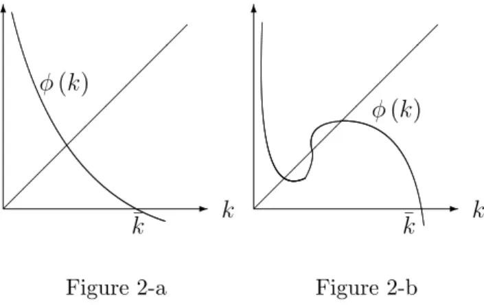
The following …gures give a graphical intuition of this proof: if (k) is con-tinuous and positive for all k 2 0; k , it is su¢ cient that lim
k!0 (k) > 0 to
have at least one equilibrium. Moreover, if there are multiple equilibria, the one with the greater ^k must verify 0 ^k < 1. Examples of unique equilibrium
and multiple equilibria are respectively presented in Figure (2-a) and (2-b). 6 - k k (k) 6 - k (k) k
Figure 2-a Figure 2-b
Derivation of …gure 1
The function c1 : [0;1) ! R with c1(0) = f (0). If n + > 0, c1 is …rst
increasing until it reaches c1(kgr)and then strictly decreasing to 1. If n+
0, c1 is strictly increasing to +1. Consider now function c2 : [0;1) ! [0; 1).
Its …rst derivative with respect of k is given by
dc2(k) dk = f0(k) (n + ) 1 1=J (f0(k) ) + kf00(k) 1 1=J (f0(k) ) f00(k) J 0(f0(k) ) [J (f0(k) )]2 k [f0(k) (n + )] [1 1=J (f0(k) )]2 (79)
Condition (20) ensures c2(0) = 0. Then, let, ^k be such that c1 k = c^ 2 k^ ;
simple manipulations of (79) show that
dc1 k^
dk
dc2 k^
dk < 0 (80)
is equivalent to 0 k^ < 1. Hence, if (21) is veri…ed, c1(k) and c2(k) cross
each other only once and …gure 1 follows.
PROOF. [Proof of proposition 4] We have de…ned ^k such that ^k = ^k; n . This proof details the simple computing that leads to (28). Application of implicit functions theorem yields
d^k dn =
0 n k; n^
Deriving equation (19) with respect to n yields 0 n(k; n) = 1 f0(k) (n + ) (k; n) (82) +f (k) kf 0(k) f0(k) (n + )[g (n) h (n (f 0(k) ))] J (f0(k) )
where J , g and h are de…ned in lemma 1. At the equilibrium such that ^k = ^
k; n one may, using equations (17) and (19), rewrite (82) such that
0 n k; n^ ^ k = J f0 ^k J f0 k^ 1 " g (n) h n f0 k^ + ^ k ^ c # (83)
where ^cstands for the aggregate consumption.
Now turn to the de…nition of the average age of capital holders using (26). Integrating by parts the numerator, using a (0) = p ( ) = 0; yields
a= 1 n R 0 ( j ) p ( ) exp ( n ) a ( ) d nR0 p ( ) exp ( n ) a ( ) d + R 0 p ( ) exp ( n ) a0( ) d nR0 p ( ) exp ( n ) a ( ) d (84)
Replace condition (2) and rearrange using (59), (60) and (7) to obtain
a = 1 n 1 n r a+ g (n) w a h (n r) c a (85)
Then, since a = k and using factor prices equations, it yields
h (n r) = (f0(k) (n + )) a k c + g (n) f (k) kf0(k) c + k c (86) Replace (86) in (83) and arrange, using (57) and recalling that g (n) = w, to
obtain
0
n ^k; n = k [^ a w] (87)
replace in (81); this yields (28).
PROOF. [Proof of proposition 5] We demonstrate it exists a n that solve
0
with 0n de…ned by (83). Let be such that f0 k = + . Since there is no
restrictions on n at the equilibrium, it is su¢ cient for the existence of n to show that: (i) 0n is continuous in n; (ii) 0n ^k; n < 0 for all n > ; (iii)
lim
n! 1 0
n ^k; n > 0 (89)
(i) To show the continuity of 0nin n, we simply have to prove that 0n(kgr; n)
1 when kgr < k. Indeed, observe with (65) and (68) that both numerator and
denominator of (83) equal zero, for ^k = kgr. Applying l’Hôpital’s rule yields
lim ^ k!kgr 0 n k; n =^ kgr h ((1 ) n) g (n) (90) 8 > < > : h0((1 ) n) [g (n) h ((1 ) n)]2 +f00(k1gr) d dk kgr f (kgr) kgrf0(kgr) 9 > = > ;
which, using (67) and (73) and recalling that h0 < 0, is negative and …nite.
(ii) Inequality n > is equivalent to kgr < k. Hence note with (83) that since
^
c = f ^k (n + ) ^k (91)
we have to prove that
h n f0 k^ g (n)
^ k
f ^k (n + ) ^k , ^k k
gr (92)
Recall with (68), that the equality between the two terms of (92) is guaranteed when ^k = kgr. Then, observing that the left hand side is decreasing in ^k (because h0 < 0) and that the right hand side is increasing in ^k, is su¢ cient
to prove that (92) always holds.
(iii) Recall …rst (lemma 1) that
lim n! 1g (n) = limn! 1h n f 0 ^k = (93) Hence, with (83) lim n! 1 0 n k; n = lim^ n! 1 ^ k f0 k^ (n + ) (94)
PROOF. [Proof of proposition 6] This is proven by the point (ii) of the proof of proposition 5.
PROOF. [Proof of proposition 7] As a preliminary, let us denote 0n ^k; n;
the …rst derivative of (34) with respect to n; the same kind of computations as those done in the proof of proposition 4 yield that
0 n ^k; n; ^ k = J f0 k^ J f0 ^k 1 " g (n ) h n f0 ^k + ^ k ^ c # (95) where ^c = f ^k (n + ) ^k. Hence, we de…ne n such that
0
n ^k; n ; = 0 (96)
To show that dn =d > 0, we demonstrate that @ @n 0 n k; n ;^ < 0 (97) and that @ @ 0 n ^k; n ; > 0 (98)
Condition (97) is trivial since 0n is continuous in n and since it is assumed there exists a unique n . If there are multiple solutions to (96), one should consider the one that maximizes ^k and the result would be the same.
To prove condition (98), derive (95) when n = n (i.e. when 0n k; n ;^ = 0) to obtain @ @ 0 n ^k; n ; = k^ J f0 k^ J f0 ^k 1g 0(n ) (99)
which is positive because g0 < 0 (lemma 1) and J > 1 for all n < . This
establishes the proof.
References
[1] A.B. Abel, The e¤ects of a baby boom on stock prices and capital accumulation in the presence of social security, Econometrica 71 (2003), 551-578.
[2] B.W. Arthur, G. McNicoll, Optimal time paths with age-dependence: a theory of population policy, Rev. Econ. Stud. 44 (1977), 111-123.
[3] B.W. Arthur, G. McNicoll, Samuelson, population and intergenerational transfers, Int. Econ. Rev. 19 (1978), 241-46.
[4] O. Blanchard, Debt, de…cits and …nite horizons, J. Polit. Economy 93 (1985), 223-247.
[5] A. Bommier, R.D. Lee, Overlapping generations models with realistic demography: statics and dynamics, J. Population Econ 16 (2003), 135-160. [6] R. Boucekkine, D. de la Croix, O. Licandro, Vintage human capital,
demographic trends and endogenous growth, J. Econ. Theory 104 (2002), 340-375.
[7] W.H. Buiter, Death, population growth and debt neutrality, Econ. J. 98 (1988), 279-293.
[8] J.L. Burke, Equilibrium for overlapping generations in continuous time, J. Econ. Theory 70 (1996), 364-390.
[9] D. Cass, Optimum growth in an aggregative model of capital accumulation, Rev. Econ. Stud. 32 (1965), 233-240.
[10] D. Cass, M.E. Yaari, Individual saving, aggregate capital accumulation, and e¢ cient growth, in: K. Shell (Ed.), Essays on the Theory of Optimal Economic Growth, MIT Press, Cambridge, MA, 1967, pp. 233-268.
[11] D. de La Croix, P. Michel, A Theory of Economic Growth: Dynamics and Policy in Overlapping Generations, Cambridge University Press, Cambridge, 2002. [12] S. Demichelis, H. Polemarchakis, Frequency of trade and the determinacy
of equilibrium paths: logarithmic economies of overlapping generations under certainty, Econ. Theory, forthcoming.
[13] P.A. Diamond, National debt in a neoclassical growth model, Amer. Econ. Rev. 55 (1965), 1126-1150.
[14] J.D. Geanakoplos, H.M. Polemarchakis, Overlapping generations, in: W. Hildenbrand, H. Sonnenschein (Eds.), Handbook of Mathematical Economics, North-Holland, New York, 1991, pp. 1899-1960.
[15] F. Duc, C. Ghiglino, Optimality of barter steady states, J. Econ. Dynam. Control 22 (1998), 1053-1067.
[16] M. Feldman, C. Gilles, An expository note on individual risk without aggregate uncertainty, J. Econ. Theory 35 (1985) 26-32.
[17] D. Gale, Pure exchange equilibrium of dynamic economic models, J. Econ. Theory 6 (1973) 12-36.
[18] C. Ghiglino, M. Tvede, No-trade and uniqueness of steady states, J. Econ. Dynam. Control 19 (1995), 655-661.
[19] C. Ghiglino, M. Tvede, Dynamics in OG economies, Journal of Di¤erence Equations and Applications, 10 (2004), 463-472.
[20] J.M. Grandmont, Money and Value: a Reconsideration of Classical and Neoclassical Monetary Theories, Cambridge University Press, Cambridge, 1983. [21] K. Judd, The law of large numbers with a continuum of i.i.d. random variables,
J. Econ. Theory 35 (1985), 19-25.
[22] T.J. Kehoe, Multiplicity of equilibria and comparative statics, Q. J. Econ. 100 (1985), 119-147.
[23] H. Konishi, F. Perera-Tallo, Existence of steady-state equilibrium in an overlapping-generations model with production, Econ. Theory 9 (1997), 529-537.
[24] T.C. Koopmans, On the concept of optimal economic growth, in: The Econometric Approach to Development Planning, North Holland, Amsterdam, 1965.
[25] J. Laitner, The dynamic analysis of continuous-time life-cycle savings growth models, J. Econ. Dynam. Control 11 (1987), 331-357.
[26] R.D. Lee, Age structure, intergenerational transfers and economic growth: an overview, Revue Econ. 31 (1980), 1129-1156.
[27] A.J. Lotka, Théorie analytique des associations biologiques, Hermann et Cie, Paris, 1939.
[28] E. Malinvaud, Macroeconomic theory, in: C.J. Bliss, M.D. Intriligator (Eds.), Advanced Textbooks in Economics 35, Elsevier, 1998, Vol. A, Chap. 2.
[29] P. Michel, P. Pestieau, Population growth and optimality: when does serendipity hold?, J. Population Econ. 6 (1993), 353-362.
[30] J.M. Poterba, Demographic structure and assets returns, Rev. Econ. Statist. 83 (2001), 565-584.
[31] P.A. Samuelson, The optimum growth rate of a population, Int. Econ. Rev. 16 (1975), 531-538.
[32] A. Seierstad, K. Sydsæter, Optimal control theory with economic applications, in: C.J. Bliss, M.D. Intriligator (Eds.), Advanced Textbooks in Economics 24, North-Holland, 1987.
[33] J. Tobin, Life cycle saving and balanced growth, in: W. Fellner (Ed.), Ten Economic Studies in the Tradition of Irving Fischer, Wiley, New York, 1967, pp. 231-256.
[34] P. Wang, Money, competitive e¢ ciency, and intergenerational transactions, J. Monet. Econ. 32 (1993), 303-320.
[35] R. J. Willis, Life cycle, institutions, and population growth: a theory of the equilibrium interest rate in an overlapping generation model, in: R.D.Lee, W.B. Artur, G. Rodgers (Eds.), Economics of Changing Age Distributions in Developed Countries, Clarendon Press, Oxford, 1988, pp. 106-138.
[36] P. Weil, Overlapping families of in…nitely-lived agents, J. Public Econ. 38 (1989) 183-198.
[37] M.E. Yaari, Uncertain lifetime, life insurance and the theory of the consumer, Rev. Econ. Stud. 32 (1965), 137-150.