HAL Id: inria-00124874
https://hal.inria.fr/inria-00124874
Submitted on 16 Jan 2007
HAL is a multi-disciplinary open access
archive for the deposit and dissemination of
sci-entific research documents, whether they are
pub-lished or not. The documents may come from
teaching and research institutions in France or
L’archive ouverte pluridisciplinaire HAL, est
destinée au dépôt et à la diffusion de documents
scientifiques de niveau recherche, publiés ou non,
émanant des établissements d’enseignement et de
recherche français ou étrangers, des laboratoires
model transformations
Charles André, Frédéric Mallet, Marie-Agnès Peraldi-Frati
To cite this version:
Charles André, Frédéric Mallet, Marie-Agnès Peraldi-Frati. Non-functional property analysis
us-ing UML2.0 and model transformations. [Research Report] RR-5913, INRIA. 2006, pp.18.
�inria-00124874�
a p p o r t
d e r e c h e r c h e
INSTITUT NATIONAL DE RECHERCHE EN INFORMATIQUE ET EN AUTOMATIQUE
N° 5913
Mai 2006THÈME COM
Non-functional Property Analysis using UML2.0 and
Model Transformations
Unité de recherche INRIA Sophia-Antipolis 2004, route des Lucioles, 06902 Sophia-Antipolis (France) Téléphone : +33 (0)4 92 38 77 77 – Télécopie : +33 (0)4 92 38 77 65
Non-functional Property Analysis
using UML2.0 and
Model Transformations
C. André
1, F. Mallet
2M-A. Peraldi-Frati
3Thème COM – Systèmes communicants Projet AOSTE
Rapport de recherche n° 5913 – Mai 2006 – 18 pages
Abstract: Real-time embedded architectures consist of software and hardware parts. Meeting non-functional constraints (e.g., real-time constraints) greatly depends on the mappings from the system functionalities to software and hardware components. Thus, there is a strong demand for precise architecture and allocation modeling, amenable to performance analysis.
The report proposes a model-driven approach for the assessment of the quality of allocations of the system functionalities to the architecture. We consider two technical domains: the UML domain for the definition of the model elements (for both description and analysis), and an analysis domain, external to UML, used for formal verification. This report defines three meta-models—one for each domain—and provides automated transformations within and between these domains. A special attention is then paid to temporal property analysis, based on a particu-lar analysis model: the Moduparticu-lar and Hierarchical Time Petri Nets.
Keywords: Model transformation, UML2.0, Non-functional property analysis, Distributed em-bedded systems, Time Petri Net.
1
I3S Laboratory (CNRS/UNSA/INRIA) Sophia Antipolis (F)– [email protected] 2
I3S Laboratory (CNRS/UNSA/INRIA) Sophia Antipolis (F)– [email protected] 3 I3S Laboratory (CNRS/UNSA/INRIA) Sophia Antipolis (F)– [email protected]
UML2.0 et Transformation de Modèles pour l’Analyse
de Propriétés non Fonctionnelles
Résumé: Les architectures embarquées sont composées de parties logicielles et matérielles. Le respect des contraintes non fonctionnelles, telles que les contraintes temporelles, dépend gran-dement de la projection des fonctionnalités du système sur des composants qui peuvent être ma-tériels ou logiciels. Aussi existe-t-il une forte demande des concepteurs pour modéliser précisé-ment l’architecture et l’allocation et faire ensuite de l’analyse de performance. Ce papier pro-pose une approche orientée modèle pour évaluer la qualité de l’allocation des fonctionnalités sur l’architecture. Deux domaines techniques sont considérés: le domaine UML pour la définition des éléments du modèle (de description et d’analyse), et le domaine d’analyse, externe à UML utilisé pour la vérification formelle. Ce rapport définit trois méta-modèles, pour chacun des do-maines, et propose les règles de transformations entre modèles. Une attention particulière est portée sur l’analyse des propriétés temporelles en se basant sur le modèle des réseaux de Petri temporisés hiérarchiques et modulaires
Mots clés: Transformation de Modèles, UML 2.0, Analyse de propriétés non fonctionnelles, systèmes embarqués répartis, Réseaux de Petri temporels.
1
Introduction
Real-time embedded architectures consist of software and hardware parts. Meeting non-functional constraints (e.g., real-time constraints) greatly depends on the mappings from the system functionalities to software and hardware components. Such a mapping—here called allo-cation—includes temporal scheduling as well as spatial partitioning and communication synthe-sis aspects. Thus, there is a strong demand for precise architecture and allocation modeling, amenable to performance analysis and that captures the heterogeneous nature of architectures and applications.
This report addresses this problem and describes a model-based solution with a special focus on allocation and its impact on system operational properties. This implies defining domains, their associated metamodels and transformations. UML 2.0 [1] with its extension capabilities (pro-files) is a good candidate for modeling. For real-time embedded applications—such as data and image processing, and automatic control—functionality and expected behavior are often speci-fied by data flow models. This justifies our choice of the UML 2.0 activities for behavioral modeling. On the other hand, SysML [2][3] has introduced two concepts: block and allocation. A block is a modular unit that may include both structural and behavioral features. The term allocation denotes the organized mapping of elements within the various structures and hierar-chies of a user model. The Deployment concept supported by UML is a special case of alloca-tion.
In our proposal, we reuse a subset of UML 2.0 and we provide extensions, often inspired from SysML. UML activities are extended to support the synchronous reactive model of computa-tion [4] that is suitable for the kind of real-time applicacomputa-tions we target: applicacomputa-tions with pre-dictable inputs, quasi periodic and where the use of a real-time operating system is forbidden by the small amount of resources available. UML activities enriched with allocation information are then transformed into a block-based model convenient for our property verification mecha-nisms. Both models are defined by a metamodel that specifies well-formedness rules. Structural transformation rules are also provided. Thus, from a behavioral description of the application and information on the architecture and the potential deployments of operations, an analysis model can be automatically derived, by model transformations. In this report, several intermedi-ate models are given for illustrative purpose. Most of them are purely internal representations, automatically generated by a chain of transformations. They should be used only by tools, and in no case drawn by the user.
The semantics of the final model is beyond the scope of the UML. In this report, since timing properties are studied, we have chosen Time Petri Nets. The model interpretation and the prop-erty verification techniques applied are relevant to the Petri Net Domain [5]. This domain is mathematically well-founded and dedicated property-checking tools are widely available.
Related works
Some aim at giving a more precise semantics to UML. The standard semantics of UML such as explained by Selic [6] is very general even though there were some attempts to give a more pre-cise semantics [7]. When addressing a specific domain, a subset of UML is often sufficient but may require a formal semantics. For instance, in the UML specification, activities use an infor-mal semantics inspired from Petri-Net. A forinfor-mal definition of the semantics of the activities in terms of Petri-nets has been proposed [8] by introducing one-to-one structural transformations. When considering time behavior, the model needs further extensions. Such is the TURTLE (Timed UML and RT-LOTOS Environment) approach [9]. It proposes the expression of temporal requirements through extended UML2.0 interaction and sequence diagrams. TURTLE is specific
to real-time embedded systems design and provides a formal framework based on the RT-LOTOS language. The automatic generation of RT-LOTOS code allows for formal analysis of this design by using the RTL tools.
The standardization of domain-specific extensions for UML has to follow a profile submission process. For instance, in the domain of real-time systems, the UML profile for Schedulability, Performance and Time defines standard paradigms of use for modeling of time, schedulability and time-related aspects [10]. This profile is being revised and should be merged into some fu-ture extensions [11].
In this report, we attempt to define a mapping for a restricted-class of activity diagrams to Time Petri Nets. We do not aim at specifying a full simulation semantics for the activity but rather to provide a support for verifying non functional properties (like deadline information) on activi-ties. Hence, as an example, we provide one-to-many transformation rules that only capture the temporal information extracted from the activity diagram and according to some allocation con-straints. Other non functional properties would induce other transformation rules.
The report structure reflects the chain of modeling and transformations. Section 2 presents an application specification. The next section introduces specialized UML activities for the behav-ioral modeling and data flow representation. Section 4 defines our analysis metamodel and the transformation from activities to structure; the resulting model is annotated with information about potential allocations. Section 5 is devoted to an original property-checking technique: timing properties studied by the automatically derived Time Petri nets.
2
Application Specification
2.1
Algorithm/Architecture
This example is a simplified version of a control and signal processing application. Operations stand for complex atomic data processing. This is a TLM (Transaction Level Model [12]) de-scription where an operation may be an IP (Intellectual Property) such as an FFT, a convolution, a filtering… Usually these applications are executed in a cyclic and periodic way. During a cy-cle, sensors are read, operations are performed and outputs are issued.
This application consists of 4 input signals (M, A, B, C, from sensors), 3 output signals (W, Y, Z, to actuators) and 3 operations (oper1 to oper3). From the functional point of view, the system may operate in two modes (M1, M2) selected by the input M. Each mode is specified by a data flow model. A functional specification of the expected behavior is:
1( )
if
1
2( )
3(
1( ),
2( )) otherwise
W
oper C
M
M
Z
oper C
Y
oper oper A oper
B
=
=
=
=
The execution platform is given: 2 processors (P1 and P2) connected by a bidirectional channel. This example is often used as an illustration of the SynDEx AAA methodology [13] that focuses on the adequation between algorithm and architecture (timeliness and optimization). Even though the goal is the same, our approach is different because it follows the MDA (Model Driven Architecture) flow suggested by the OMG and use an UML activity as an input while SynDEx use its own format. We rely on UML 2.0, existing profile (Schedulabitity,
Perform-ance, and Time specification: SPT [10]) and forthcoming profiles (system engineering [14], Marte [11]).
2.2
Non functional constraints
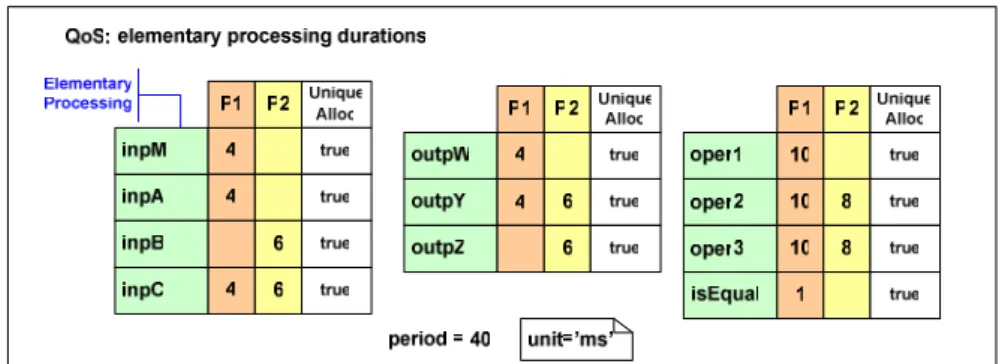
Various non functional constraints are imposed. Deadline is such a constraint (a period of 40 time units, equal to the deadline): whatever the mode, all operations must be executed within this deadline. Other constraints are related to deployment: some processing elements have fixed location; others have to be mapped onto physical resources so that real-time constraints are met.
Figure 1: Execution durations for processing elements.
With the knowledge of the performances of the platform elements (processors and channels), a cost specification can be associated with pairs “processing, processor”, and “communication, channel”. For instance, the cost can be an execution time characterized by a time interval, possi-bly reduced to a single value as in Figure 1. Additional allocation constraints can be specified such as uniqueness of deployment, expressed by the uniqueAllocation attribute. In our example,
oper2 is potentially deployable on P1 or P2, but since uniqueAllocation is true, we may choose to
allocate oper2 either on P1 or P2, but not both.
Note that, in Figure 1 inpX (outpX) stands for the acquisition (actuation) processing of signal X.
Inter processor communications have a duration that depends on the type of transmitted data (Figure 2, left-hand side). More generally, several channels (e.g., Ethernet and WiFi) may exist between two processors, associated with different costs (Figure 2, right-hand side). The commu-nications may even be dissymmetric (e.g., ADSL where upstream and downstream communica-tion costs are different).
3
Data flow representation
In UML 1.x activity graphs were just an informal specialization of state machines. Such a repre-sentation was not convenient for systems engineers. To address this issue, explicit reprerepre-sentation of data and control flows has been introduced through activity diagrams. Now, in UML 2.0, activities are first class concepts with their own diagrams. The semantics of activities is large enough to cover several domain-specific interpretations [6]. A more precise semantics can be given in profiles using the semantics variation points. In our case, the semantics is implied by the systematic structural transformations performed that lead to a mathematically well-founded model, the Time Petri nets.
An activity is a UML behavior. It specifies a partial ordering of executions of subordinate be-haviors, using control and data flow models. Activity diagrams support hierarchical description; subordinate behaviors are individual elements (actions) that can be invocation actions or struc-tured activity nodes. The UML::Activities package consists of many packages. In order to provide automated transformations, we do not support all the activity model elements and constructs. Moreover, since our activities represent synchronous reactions, we consider only acyclic activi-ties. These kinds of restrictions can be imposed by stereotyping. So, we define «sActivity», a stereotype of Activity.
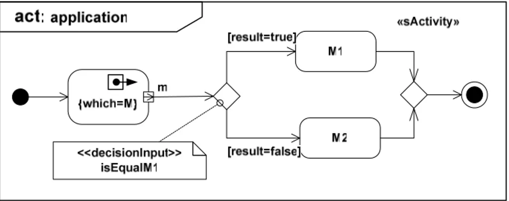
Figure 3: Activity Diagram (top-level).
Figure 3 represents the application activity at the top level. Modes are selected by a
Decision-Node. A DecisionInput is a behavior attached to a decision node, which selects one of its outgoing
Figure 4 : Refinement of the DecisionInput.
The decision node is refined into an invocation action (decision), defined by its own activity diagram (
Figure 4). Here, an action is a UML CallBehaviorAction that directly invokes a behavior. In our approach, the behavior is either elementary (e.g., isEqual, and thus specified by an elementary operation given in a table, see Figure 1) or further refined as an activity diagram (e.g.,
isE-qualM1).
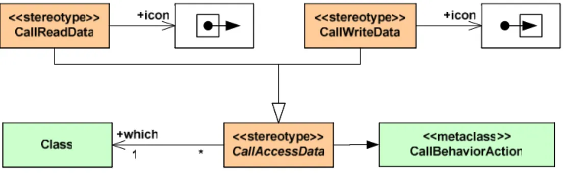
Access to information demands special actions, which can be resource and time consuming. We explicitly represent these accesses using two stereotypes of CallBehaviorAction: CallReadData for inputs and CallWriteData for outputs. They are defined in
Figure 5. The “which” stereotype attribute refers to the entity that conveys the value. This is a constant reference, not implying any object flow, and assigned to a ValuePin.
Figure 5: Data Access Stereotypes.
Actions M1 and M2 are call behavior actions, specified in separate activity diagrams. Activity M1
is described in Figure 6 and M2 in Figure 7.
Figure 7: Activity Diagram (Mode M2).
Since activities are behaviors, their instances are UML executions. To be able to perform formal property verifications on our model we need a more precise semantics. We use a synchronous semantics such as defined in synchronous languages. This semantics is well adapted to the kind of applications we focus on.. This choice requires this approach to be restricted to applications with deterministic executions or at least to applications for which a valid deterministic behavior can be derived. A synchronous system evolves in a sequence of non overlapping reactions in a lock-step manner. A typical synchronous execution scheme consists of a read phase (input ac-quisitions), a computation phase and finally, a write phase (actuation). The sequence of these three phases is called a reaction and must be performed in isolation. Moreover a synchronous execution is finite, it is loop-free and deterministic. Details about synchronous execution seman-tics are beyond the scope of this report (see [15]). An important consequence of the synchronous execution hypothesis is that an SActivity diagram is a Directed Acyclic Graph (DAG).
4
From Data flow to Structure
Activity diagram focuses on the execution with a strong flow flavor and applies well to engi-neering systems. An activity expresses what to do but little where to do it. Furthermore an activ-ity is not very well suited to represent communications. Activactiv-ity partitions (and swimlanes) are helpful in indicating responsibilities in a system. They could also be used to indicate where ac-tions take place. However, this approach is not convenient to express multiple potential alloca-tions. A block-based description is a better solution. SysML has adopted such a point of view with its blocks (formerly named assemblies). A block diagram is a modular description that combines both structure and (data and control) flows.
As communication is essential in distributed systems, we choose to reify it as a specialized communication block, thus making explicit communication media induced by the distribution. This departs from the classical representation of communication as activity edge in activity dia-grams, or as connector in composite structure diagrams. We propose an analysis model made of blocks and allowing for modular descriptions. This facilitates automated transformations and reuse of components from libraries.
In what follows, the diagrams that illustrate the model transformations are not to be drawn by the user. They are just diagrammatical representations of an XMI file used by tools.
4.1
Analysis Metamodel
Figure 8 contains the Analysis metamodel. Analysis blocks are UML structured classes that own analysis ports (a stereotype of UML ports). Ports are connected by UML connectors. An analy-sis port is either an input port or an output port (according to the value of its direction attribute). An analysis model is made of processing blocks; one of them is the top. A processing block is a flat assembly of nodes: elementary processing nodes, control nodes, and reference nodes. Even
if a processing block is a flat representation, the model allows for hierarchical descriptions through the use of references. Note that an analysis block owns analysis ports, not standard ports, what is expressed by the required constraint on the extension association. The observer nodes mentioned in the AnalysisModel package are associated with properties. They instrument analysis models and are used in Section 5.
Figure 8: Analysis metamodel.
4.2
Structural TransformationFigure 9 represents a processing block automatically generated from the top-level activity (named application). It results from the model transformation described below. ibd stands for internal block diagram, phrase borrowed from SysML.
Thanks to the limitations imposed to activity models (SActivity), the transformation from Activ-ity into Analysis models is one-to-one for most of model elements (Table 1). In this table, Scat-ter and Gather are subclasses of AnalysisModel::ControlNode. They have an attribute named
mode taking values in {or, and}. The type Ctrl is a predefined type, standing for control. There are the block counterparts of fork, decision, join and merge nodes.
Activity model element Analysis model element
SActivity ProcessingBlock
ActivityEdge Connector
Fork, Decision Scatter
Join, Merge Gather
InitialNode AnalysisPort {type=Ctrl}
ActivityParameterNode AnalysisPort
Table 1: Model element transformation.
Some model elements require adding explicit communications. Communications are represented as a subclass of ElementaryProcessingNode named CommunicationNode. In processing block dia-grams, communications are drawn as pipes. Communications must explicitly appear when they may have a cost. To avoid duplication, communications are systematically inserted before the use of the item flow by a processing element, represented as a subclass of ElementaryProcessing-Node named ProcessingNode.
An elementary operation is transformed into a ProcessingNode (denoted «pn»), preceded by a communication for each of its input ports. Other operations, whose behavior is defined in a separate activity diagram, are transformed into reference nodes (denoted «refn» and drawn with a dashed outline). No communication is inserted for a ReferenceNode. Its ports are virtual (the
is-Virtual attribute is asserted) and communication costs are paid only when used by processing
nodes defined within the referenced processing block.
An ActivityFinalNode also needs a special transformation. It is always translated into an output
control analysis port. A communication is inserted only for the top-level processing block.
Remark 1: To sum up, communications are present only before processing nodes, and before the output port of the top-level processing block.
Remark 2: An SActivity diagram is a directed acyclic graph. Our transformation preserves directedness that is manifested by port direction, and acyclicity. Therefore, an ibd can be consid-ered as a DAG.
Figure 9 and Figure 10 illustrate this transformation for the top-level activity (named applica-tion), and for activity M1 (M2 is similar and has been omitted). Remind that these diagrams are not to be drawn by the user. There are just diagrammatical representations of XMI files used by tools.
Figure 9: Processing Block (top-level)
Figure 10: Processing Block (M1).
4.3
Potential Allocation
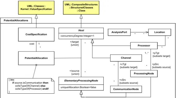
Processing and communication costs are related to a pair “elementary processing element, host”. A host can be either a processor or a channel. In our metamodel (Figure 11), this is represented as an association class named PotentialAllocation. An elementary processing node, associated with an elementary operation, can be potentially deployed onto several targets. This target is a set of processors represented by the pTgt association end. For instance, oper3 can be deployed on proc-essors P1 or P2. Respective costs are given in tables from Figure 1. Analysis ports are associated with a set of potential allocations on processors (i.e., a set of sets of processors). The cost
asso-ciated with a processing block results from a semantic transformation that propagates allocation information. This process is explained below.
AnalysisPort uniqueAllocation:Boolean=false ElementaryProcessingNode UML::CompositeStructures ::StructuredClasses ::Class concurrencyDegree:Integer=1 Host +/target {union} +/source {union} * * PotentialAllocation CostSpecification cost * 1 UML::Classes:: Kernel::ValueSpecifcation { inv: if source.isCommunication then oclIsTypeOf(Channel) else oclIsTypeOf(Processor) endif } PotentialAllocations Processor Channel ProcessingNode CommunicationNode 1..* * +pSrc{subsets source} +pTgt {subsets target} * * +cSrc{subsets source} +cTgt {subsets target} Location * * * *
Figure 11: Potential Allocation.
4.4
Full characterization of potential allocations
Objective: Given the potential allocations for all elementary operations, derive all potential communications from the analysis model.
Let P be the set of processors of the application. A location L is a set of sets of processors:
( )
L
⊂℘
P
. For instance, forP
=
{
P P P P
1,
2,
3,
4}
,l
=
{
{
P P
1,
2} { }
,
P
3}
∈
L
. Location l is interpreted as: either P3 or (P1 and P2 together). We define two operations on L: the disjunctiveand the conjunctive products:
{
}
{ }
k=n k=1 k=n k=1:
such that
|
,
1..
:
such that
|
,
1..
n k k n j j k k k k kL
L
l
s s
l k
n
L
L
l
s
s
l k
n
⊕
→
=
∈
=
⊗
→
=
∈
=
⊕
⊗
∪
For
l
1=
{
{
P P
1,
2} { }
,
P
3}
and
l
2=
{
{
P P
1,
3}
}
,l
1⊕ =
l
2{
{
P P
1,
2} { } {
,
P
3,
P P
1,
3}
}
and{
} {
}
{
}
1 2 1
,
2,
3,
1,
3l
⊗ =
l
P P P
P P
The notation of locations as set of sets is especially clumsy. Henceforth, we denote them as for-mal sums. For instance, l1 and l2 of the above example are denoted
l
1=
P P
1i
2+
P
3 and1 3
2
l
=
P P
i
, respectively, andl
1⊕ =
l
2P P
1i
2+ +
P
3P P
1i
3,l
1⊗ =
l
2P P P
1i
2i
3+
P P
1i
3. In our metamodel a communication node owns one input port (Pi) and one output port (Po). LetLi=Pi.location and Lo=Po.location. The Cartesian product Li×Lo yields the set of pairs (source,
(
)
{
}
2 1 2 1 2:
L
L
such that
l
l
s s
,
|
s
kl k
k,
1..2
×
→
× =
∈
=
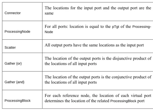
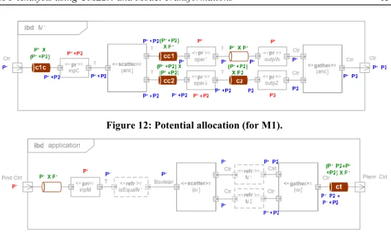
To respect these rules the following constructive process is proposed. The full characterization of potential allocations is done by a traversal of the processing blocks, starting with the top level, and exploring nodes according to an order obtained by performing a topological sorting on each processing block. Remark 2 of Section 4.2 ensures that the topological order always exists. The user gives the locations for the initial and the terminal ports of the top-level process-ing block. While traversprocess-ing the graph, port locations are propagated in a consistent way with some invariant relations (Table 2). Non respect of these rules will result in an ill-formed analysis model. Figure 12 and Figure 13 display the resulting allocations for the processing block M1 and the Application processing block (allocation for M2 has been omitted).These figures take into account allocation constraints expressed in Figure 1 and Figure 2. From the Cartesian products associated with the communication nodes we deduce potential allocations: c13 onto {Ch1_1, Ch1_2}, and c23 onto {Ch1_1, Ch1_2, Ch2_1, Ch2_2}. If there were several channels between two processors (as in Figure 2, right-hand side), the potential allocation for c13 will be {Ch1_1, Ch1_2.w, Ch1_2.e}.
Connector
The locations for the input port and the output port are the same
ProcessingNode
For all ports: location is equal to the pTgt of the Processing
-Node
Scatter All output ports have the same locations as the input port
Gather {or}
The location of the output ports is the disjunctive product of the locations of all input ports
Gather {and}
The location of the output ports is the conjunctive product of the locations of all input ports
ProcessingBlock
For each reference node, the location of each virtual port determines the location of the related ProcessingBlock port
Figure 12: Potential allocation (for M1).
Figure 13: Potential allocation (for Application).
5
From Structure to Temporal Analysis
5.1
Hierarchical and Modular Time Petri Nets
Our main goal is to formally verify some non functional properties of the application. In this report, we focus on time properties. For this purpose, we need to fulfill three requirements. First, give a formal semantics to the intended behavior of each analysis node. Second, compute the behavior of processing blocks by composing the behavior of contained nodes. Third, express properties to be verified.
To address the first requirement, Time Petri nets [16] have been preferred to the UML State Machines and Activities. Petri nets have well-established mathematical foundations (semantics) and offer rich analysis capabilities. Contrary to UML state machines, Petri nets support true concurrency. As for UML2.0 activity diagrams, though they are inspired from Petri nets, they lack a formal semantics.
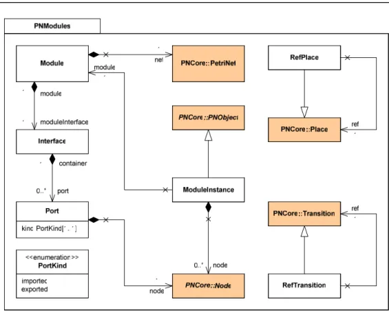
Figure 14: Modular Time Petri Net Model.
Modular and hierarchical Place/Transition nets (MHTPN) meet the second requirement, mak-ing it possible to compose behaviors. The Petri Net community is workmak-ing on a model generic enough to cover all Petri Net formats (namely, the Petri Net Markup Language [17]). In the con-text of our work a less general model—closer to our previous UML-based models—is sufficient (Figure 14). This hierarchical model is built upon the classical flat model of Petri nets (Figure 15). In this latter model, timing information (a special kind of cost specification) is attached to transition (Time Petri Net).
To satisfy the last requirement, we choose an observer node or a special control node (Figure 8); the former for properties like deadline, the latter for constraints.
PetriNet PNObject labelNode: EString[1..1] Node capacity:EInt[0..1] tokenLoad: EInt[1..1] Place Transition kind: ArcKind[1..1] weight: EInt[1..1] Arc pre post <<enumeration>> ArcKind includesMin: EBoolean[1..1] includesMax:EBoolean[1..1] lowerBound:EInt[1..1] upperBound:Eint[1..1] TimeInterval pNObject net 1 0..* arc place 1 0..* 0..* 1 transition arc timeInterval 0..1 PNCore
Figure 15: Time Petri Net Core Model.
The Petri Net analysis tool named Tina [16] supports both timed and untimed nets. However, it does not support hierarchical descriptions. We have built a tool that allows for graphical compo-sition of Petri Net modules. It exports flattened modules into a Tina-compatible format.
Figure 16: Petri net elements library.
5.2
Model Transformation
The goal is to derive a MHTPN from an analysis model and additional information (e.g., con-straints, properties). This transformation is made easier by the use of blocks, each of which be-ing transformed into a module. Table 3 contains mappbe-ing rules.
Analysis model element PN model element
ProcessingBlock (toplevel) PetriNet
ProcessingBlock (others) Module
AnalysisNode ModuleInstance Host Place Host::concurrencyDegree Place::tokenLoad Place::capacity Port Port PotentialAllocation::cost TimeInterval
Table 3: Analysis model element transformation.
We have defined a library of modules that are instantiated (as ModuleInstance). Table 4 shows examples of mappings from analysis nodes to Petri net library modules. Modules are parameter-ized and can be specialparameter-ized in so as much as the interface is preserved.
Analysis nodes PN Library Modules
ElementaryProcessingNode ProcessingElement (PE)
Scatter Fork, Choice
Gather Join, Merge
ObserverNode ObservingElement (OE)
Table 4: Petri net library elements.
5.3
Software environment
We have started to implement a tool suite in Java that supports all transformations. To be con-sistent with UML models, usually described in XML using the XMI format, all our models (in-cluding transformation models) are described in XML. The grammars of our XML files are de-scribed using XML Schema (whereas the original PNML format is specified in a RelaxNG schema). Java provides technologies for managing XML and XML schema, for applying model transformations, and for binding XML schema elements to Java classes. Unfortunately, there are three technological limitations that still prevent us from having a fully integrated tool suite. First, these technologies are evolving very quickly and are not always consistent with each oth-ers. Second, we have not yet found a model transformation technology that really allows for semantics transformation, most of technologies only work with simple syntactic transformations. Third, since we use features of UML2.0, we need the XMI description of the UML2.0 meta-model (at least the subset that includes everything we use plus our own extensions). It is almost impossible to find, in the public domain, an XMI description of the UML2.0, each tool vendor apparently using its own specialized description. Finally, we do not aim at producing a complete tool suit, we only build simple academic tools to demonstrate the feasibility of our mechanisms. Thus, our tool suite is not yet complete and some steps are still performed manually.
Nevertheless, the manipulation of modular and hierarchical time Petri nets is operational. We use the Java Architecture for XML Binding 2.0 (JAXB) for binding XML schemata to Java classes and the Java Architecture for XML Processing 1.3 (JAXP) for processing XML docu-ments and applying model transformations.
Our tool expands MHTPNs to a flat model, which is a prerequisite for the time Petri net ana-lyzer (Tina). Tina generates various state space abstractions for Time Petri nets (state class graphs) and reports dead transitions. Our Petri net library modules are devised so as dead transi-tions reveal property violatransi-tions or structural inconsistency. For example, we can identify impos-sible allocations, or check whether or not the deadline constraints are met. The analysis is able
to assert that there is no valid allocation with a deadline constraint less than 38 time units. To meet the strong deadline of 38 time units, oper2, oper3 and outpY must be executed on P2, while
inpC can be executed either on P1 or P2. To meet the weaker deadline constraint of 40 time units,
oper2 must be executed on P2 but there is no constraint for other potential allocations.
6
Conclusion
This report has shown a way to use UML and model transformations to derive an analysis model from a UML functional description. First, the functionality of the application is expressed as a stereotyped UML activity diagram tailored for synchronous reactive execution.. Following the model-driven approach, this model passes through a series of transformations resulting in a model amenable to formal analyses. Intermediate models are well-formed in accordance with the UML metamodels defined in this report.
For property analysis the semantics of UML 2.0 is not sufficiently precise (many semantic varia-tion points, no formal definivaria-tion). This is a deliberate choice, as explained by B. Selic in his paper on the semantic foundation of Standard UML 2.0 [5]. This report focuses on the temporal correctness of potential allocations from operations to hardware/software execution supports. Since our system has concurrent evolutions, we have chosen Petri Nets as the analysis domain and especially, modular and hierarchical time Petri nets.
Diagram interchanges and model transformations have been implemented in Java. Temporal properties are analyzed by Tina, a time Petri net analyzer. Reachability analysis tools of Tina establish the existence of a valid allocation meeting temporal constraints.
Several extensions of this approach are possible. First, more complex properties (expressed us-ing Linear Time Logic–LTL, for instance) could be formally analyzed by a model checker; Tina supplying the behavioral graph. For instance, with the given parameters, a manual graph analy-sis has shown that oper2 must necessarily be allocated to the processor P2 in order to meet the deadline.This leads to a reduction of the possible allocations to be explored. Such a procedure would benefit from being automated. Once the adequate solutions are better characterized, we may export pertinent information, extracted from UML, to other analysis tools. For instance, we could easily export the algorithm and architecture models to SynDEx for further optimization and generation of the real-time distributed code.
Second, we have demonstrated how to associate time Petri nets with our library elements. We could have used other formalisms instead. In the future, to make the best of the underlying syn-chronous hypotheses, we intend to use the industrial synsyn-chronous language Esterel [18] and its validation tools, or the Polychrony platform [19].
7
Bibliography
[1] “Unified Modeling Language: Superstructure”. V 2.0 OMG document formal/05-07-04. April 2005. http://www.omg.org/docs/formal/05-07-04.pdf
[2] SysML Submission Team. “Systems Modeling Language (SysML) Specification. V 0.98”. OMG document ad/2005-11-01. November 2005. http://www.omg.org/docs/ad/05-11-01.pdf
[3] SysML Partners. “Systems Modeling Language (SysML) Specification”. v 1.0.alpha. OMG document ad/2005-11-05. November 2005. http://www.omg.org/docs/ad/05-11-01.pdf [4] A. Benveniste, P.Caspi, S. Edwards, N. Halbwachs, P. Le Guernic, R. De Simone. “The
synchronous languages 12 Years Later”, Proc. of the IEEE, Vol.91, n° 1, pp. 64—83, 2003. [5] The Petri Nets World. http://www.informatik.uni-hamburg.de/TGI/PetriNets
[6] B. Selic. “On the Semantic Foundations of Standard UML 2.0”, SFM-RT 2004, LNCS 3185, Springer-Verlag, pp. 181-199, 2004.
[7] Tony Clark, Andy Evans, Stuart Kent, Steve Brodsky, Steve Cook, “A feasibility Study inRearchitecting UML as a Family of Languages using a Precise OO Meta-Modelling Ap-proach” version 1.0, available from www.puml.org, September 2000
[8] H. Störrle. “Semantics and Verification of Data Flow in UML 2.0 Activities.” Electronic notes in Theoretical Computer Science, 127(4), pp. 35-52, 2005.
[9] L. Apvrille, J.-P. Courtiat, C. Lohr, P de Saqui-Sannes, “A Real-Time UML Profile Sup-ported by a Formal Validation Toolkit ”, IEEE Transactions on Software Engineering, Vol 30, N° 7, pp 473-487, July 2004
[10]“UML Profile for Schedulability, Performance, and Time, version 1.1.” OMG document formal/2005-01-02, January 2005, http://www.omg.org/docs/formal/05-01-02.pdf
[11]“UML Profile for Modeling and Analysis of Real-Time and Embedded systems (MARTE) RFP”, OMG Document realtime/05-02-06, February 2005, http://www.omg.org/-docs/realtime/05-02-06.pdf
[12]L. Cai and D. Gajski, “Transaction Level Modeling: An Overview”, Proceedings of the International Conference on Hardware/Software Codesign & System Synthesis, Newport Beach, CA, October 2003.
[13]T. Grandpierre, Y. Sorel. “From Algorithm and Architecture Specifications to Automatic Generation of Distributed Real-Time Executives: a Seamless Flow of Graphs Transforma-tions”. MEMOCODE2003, Formal Methods and Models for Codesign Conference, Mont Saint-Michel, France, June 2003.
[14] “UML profile for Systems Engineering RFP”, OMG Document ad/03-03-41, September 2003, http://www.omg.org/docs/ad/03-03-41.pdf
[15]R. De Simone, C. André. “Towards a Synchronous Reactive UML subprofile?”, Interna-tional Journal on Software Tools for Technology Transfer (STTT), Springer-Verlag, ISBN=1433-2779 (Paper) 1433-2787 (Online). DOI:10.1007/s10009-005-0206-9, Decem-ber 2005.
[16]B. Berthomieu, P-O. Ribet, F. Vernadat, “The tool TINA – Construction of abstract state space for Petri net and Time Petri Nets", Int. Journal of Production Research, Vol. 42, n° 14, pp. 2741—2756. July 2004. http://www.laas.fr/tina
[17]J. Billington, S. Christensen, K. van Hee, E. Kindler, O. Kummer, L. Petrucci, R. Post, C. Stehno, and M. Weber. “The Petri Net Markup Language: Concepts, Technology, and Tools”, ICATPN 2003, Eindhoven, June 2003. http://www.informatik.hu-berlin.de/top/-pnml/download/about/PNML_CTT.pdf
[18]Esterel Studio. http://www.esterel-technologies.com
[19]P. Le Guernic, J-P. Talpin, J-C. Le Lann. “Polychrony for system design”, Journal of Cir-cuits, Systems and Computers, 12(3), pp 261-304, April 2003.