A Comparative Performance Analysis of Position
Estimation Algorithms for GNSS Localization in
Urban Areas
Bassma GUERMAH
National Institute of Posts and Telecommunications,
INPT, Morocco
Email: [email protected]
Hassan EL GHAZI
National Institute of Posts and Telecommunications,
INPT, Morocco Email: [email protected]
Tayeb SADIKI
International University of Rabat, UIR, Morocco
Email:[email protected]
Yann BEN MAISSA
National Institute of Posts and Telecommunications,
INPT, Morocco Email: [email protected]
Esmail AHOUZI
National Institute of Posts and Telecommunications,
INPT, Morocco Email: [email protected]
Abstract—Global Navigation Satellite Systems (GNSS) have become an integral part of all applications where mobility plays an important role. However, The performances of GNSS-based positioning systems can be affected in constrained environments (urban and indoor environments), due to masking of satellites by buildings and multipath effects.
In this paper, a comparative investigation on classical GNSS localization algorithms in urban areas is presented and analyzed in terms of mean squared error.
As a result, Kalman filter estimation shows the best error performance in good environments (all satellites are in direct sight). Nevertheless, in constrained environments, the kalman filter and least square method show important positioning errors because their measurement noise model is unsuitable.
Index Terms—GNSS, Urban area, Statistical filtering algo-rithm, Multipath, NLOS.
I. INTRODUCTION
Since the middle Ages, the urgent need of humans to identify its position in its environment has always been a necessity and a challenge. From the 1960s, the history of satellite navigation has begun with the development of the American GPS(Global Positioning System) and has since changed significantly until today with emergence and develop-ment of other positioning systems, such as the Russian system GLONASS and the European Galileo system.
Since these systems are used in critical domains, i.e. maritime transport and civil aviation, requiring high accuracy, the perfor-mance criteria have been established to qualify these systems. There are four criteria commonly used to qualify these per-formances [1] namely : accuracy, availability, continuity and integrity.
However, despite the high precision required for positioning systems, the satellite positioning is affected by the problems related to the signal propagation in the atmosphere, the
in-stability of clocks, the orbital error, obstacles in receiving environment and receiver noise [2]. Therefore, the errors caused by these phenomena lead sometimes to errors that could reach up to ten meters, and this affects notably the positioning accuracy.
Furthermore, the GNSS receiver uses the classical filtering methods, such as Kalman filter [3] [4], to reduce positioning error. Nevertheless, the performances of these methods can be degraded in urban environments, due to Non-Line-of-Sight (NLOS) reception and multipath interference. Hence, it is desirable that relative performance among those algorithms has to be studied in urban area. A comparative investigation on classical estimation algorithms used in GNSS receiver is presented in this paper. Mean squared error (MSE) is used as performance measure. The data is acquired in real environment (Toulouse, France).
This paper is organized as follows. In section II, a brief introduction of GNSS systems is presented. Principles of classical filtering methods used in GNSS receiver are given in Section III. Section IV presents the urban positioning problem. A performance analysis of position estimation algorithms is presented in Section V. In Section VI, we will give some recommandations to improve positioning and to adapt the position estimation algorithms for constrained environments. The final section concludes this paper and discusses future work.
II. THEGNSS SYSTEMS
Global Navigation Satellite System (GNSS) is the standard generic term for satellite navigation systems that provide autonomous geo-spatial positioning with global coverage. A GNSS allows small electronic receivers to determine their lo-cation (longitude, latitude, and height) anytime and anywhere
in the world, using the signals as transmitted by the GNSS satellites.
A. Architecture of GNSS systems
The navigation systems share a common global architecture, consisting of three segments (cf. figure 1) [5] :
• Space Segment : It consists of a set of satellites called
constellation.
• Control Segment : It monitors the constellation and
updates the satellite information. Each navigation satellite system has its own control segment composed of mea-surement and control stations spread over the globe.
• User Segment : This includes all GNSS receivers.
Fig. 1: GNSS Architecture [6].
B. The theory of the GNSS receiver functioning
The main functions of the receiver is to capture signals transmitted by satellites in view and decode the navigation message in order to compute the transit time of the signal. The ranging codes broadcasted by the satellites enable a GNSS receiver to measure the transit time of the signals and thereby to determine the range between a satellite and the user. Thus, from the information provided by the navigation mes-sage, the user position coordinates and the user clock offset are computed using trilateration method [2]. Four satellites are normally required to be simultaneously ”in view” to the receiver for 3-D positioning purposes. Therefore, in order to compute the position of the receiving antenna, the receiver must perform the following operations [7] [8]:
• Acquisition : This operation consist to identify all
satel-lites visible to the user. If a satellite is visible, the acquisition must determine the following two properties of the signal : Frequency and Code phase.
• Tracking : The main purpose of tracking is to refine the
coarse values of code phase and frequency and to keep track of these as the signal properties change over time. This step contains two parts : code tracking and carrier frequency/phase tracking.
• Navigation Data Extraction : After a successful signals
tracking, the navigation message was extracted from the received signal.
• PVT(Position, Velocity, Time) Computation : The final
task of the receiver. It consists to compute the user position, velocity and time.
C. GNSS Measurement Model
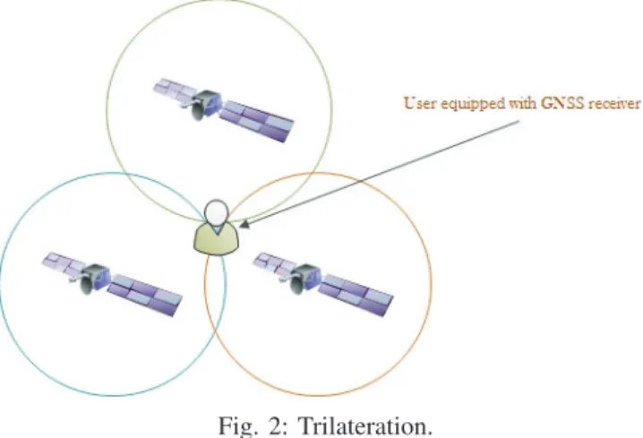
The GNSS positioning is based on trilateration method (cf.figure 2) [2]: the distance between user and satellites is measured by multiplying the travel time by the speed of light and its expressed as functions of the satellites and user coordinates. Travel time is measured by comparing the time of emission (provided by the satellite) with the time of reception (measured by the receiver). The Satellite clocks can be synchronized with a global GNSS time using information contained in the navigation message broadcasted by satellites. However, the offset between user clock and GNSS time cannot be predicted and needs to be estimated at the same time as the position. Thus, the GNSS measurement models that
Fig. 2: Trilateration.
are effectively processed by the positioning algorithm are not ranges but pseudoranges, which have the following structure :
ρst = dst− c(δtu− δts) + Its+ T s t + eph s t+ m s t + wt (1) Where :
• dst : The geometrical distance between the satellite and
the user receiver. It equals :
dst =p(xt− xst)2+ (yt− yst)2+ (zt− zts)2 • (xt,yt,zt) are the coordinates of the receiving antenna and
( xs
t,yts, zst) are the coordinates of satellite in the WGS84
standard.
• δts: The satellite clock offset.
• δtu : The receiver clock offset.
• c : The speed of light.
• Its : The Ionospheric error. • Tts : The tropospheric error. • ephst : The orbital error.
• mst : Error caused by signal reflections in constrained
environments.
In equation (1), the variables xt , yt , ztand δtuare unknown
and must be estimated by the receiver. The state vector Xt
includes all variables to be estimated and is expressed as follows :
Xt= [xt, yt, zt, c∗ δtu] (2)
III. POSITIONESTIMATIONALGORITHMS
The received signals are noisy (errors of synchronization, propagation, thermal noise of reception). Therefore, to mini-mize the impact of these noises, the receiver uses the statistical filtering techniques, which aim to estimate the state of a system from observations.
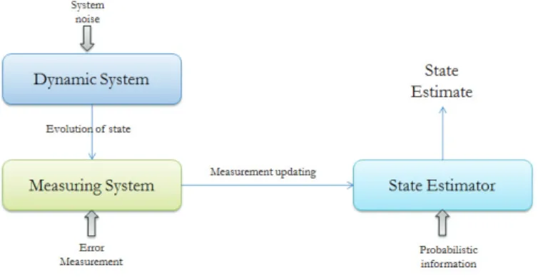
The schematization of a statistical filtering system is given by figure 3.
Fig. 3: A filtering system. The state and observation systems are defined by :
(
Xt= ft(Xt−1, Vt)
Zt= ht(Xt, Wt)
Where :
Xt : The hidden state vector.
Zt : The vector of observations.
Vt : The noise of state vector.
Wt : The noise of observations.
ftand ht : The evolution functions of state and observations.
At time t, the state evolves from Xt−1 to Xt . This evolution
of state is measured by a noisy measurement system. Thus, at
time t, we have a new measure Zt. The state estimator uses
the new measurement Zt and the probabilistic information to
estimate the state Xt and his uncertainty.
Therefore, we can note that the statistical filtering combines the available observational data and the a priori knowledge of past states for estimating the unknown state of the system. In this section we present the classical filtering methods used in GNSS receiver.
A. Least square method
The Least Square method is the most traditional method
that allows to solve the linear problems of type Y = HX + ε
in minimizing the criterion QM C(X) =k Y − HX k2.
This leads to the following estimator [9] [7] : b
X= (HTH)−1HTY (3)
For navigation systems, the observation equation is nonlinear, so, it must be linearized for applying the Least Square tech-nique.
B. The kalman filter
A Kalman filter is an optimal estimator that infers pa-rameters of interest from indirect inaccurate and uncertain observations. It is recursive so that new measurements can be processed as they arrive [3] [4]. It is subject to certain assumptions :
• Linearity of state model.
• Measurement and state noise must be white Gaussian and
uncorrelated.
Kalman filter works in a two-step process :
• The prediction step : In this step, the kalman filter
produces estimates of the current state variables, along with their uncertainties.
• The correction step : In this step, Once the outcome
of the next measurement (necessarily affected by some amount of error) is observed by algorithm, the estimates of state variables calculated in step 1 are updated using a weighted average, with more weight being given to estimates with higher certainty.
The general form of state equation of kalman filter is : (
Xt= Ft−1.Xt−1+ vt−1
Zt = Ht.Xt+ wt
Where :
Xt : The state vector at time t.
Ft−1 : The state transition matrix which applies the effect of
each system state parameter at time t-1 on the system state at time t.
vt−1 : The state noise vector.
Zt : The vector of measurement.
Ht : The transformation matrix that maps the state vector
parameters into the measurement domain.
wt : The measurement noise vector.
IV. THEURBANPOSITIONINGPROBLEM
The global navigation satellite systems suffers from many technical limitations for their use in highly degraded environ-ments (urban environenviron-ments and inside buildings) [10] [11] [12] [13] [14].
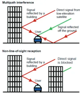
The reception of GNSS signals is disturbed by the surrounding environment of the antenna (vehicles, constructions, vegeta-tion, etc). These disturbances can be due to three phenomena : masking, multipath and NLOS reception (cf. figure 4).
• Masking : One of the major problems using the
navi-gation satellite systems in urban areas. Thus, they occur when the signal is blocked by various obstacles.
• Multipath : This phenomenon occurs when the signals
incoming from satellites can undergo reflections by ob-stacles near the antenna (buildings, walls, vehicles, and the ground). The reflected signals can interfere with the
directly received signals and take more time to reach the receiver than the direct signal.
• NLOS reception : This phenomenon occurs where the
direct signal (Line-of-sight propagation) is blocked and the signal is received only via reflection.
Fig. 4: Masking , Multipath and NLOS reception [12]. The multipath and NLOS phenomena disturb signal reception, notably, adding a delay to the propagation time. Consequently, such as the pseudorange measurements being deduced of time propagation, an additional error on pseudorange estimation will be added.
V. SIMULATIONSANDPERFORMANCEANALYSIS
Simulation has been carried out to compare and evaluate performance of classical GNSS localization algorithms. Two different scenarios are considered. The first scenario aims to estimate a trajectory for a vehicle moving in a good environ-ment using the Kalman filter and the Least Square method, and compare these two methods in terms of mean squared error. The second scenario aims to demonstrate the limits of classical filtering methods in constrained environments. For our simulations, we acquired the experimental data with a low-end receiver that shows very important pseudorange errors, since no smoothing on measure is performed and no processing to filter received signals is applied. This receiver allows as to have the raw measurements required for posi-tioning in the output files, such as satellite positions, Doppler measurements, etc. The acquisitions were taken in Toulouse for two vehicle moving respectively over a period of 3500 and 1000 seconds (cf. figure 5) along two different path, but in the same environment. The data is computed out in collaboration with ISAE/SUPAERO University of Toulouse. Pseudorange measurements are obtained from approximately seven satellites.
(a) Trajectory over a period of 3500 seconds
(b) Trajectory over a period of 1000 seconds
Fig. 5: Reference trajectories.
A. Scenario 1:
The simulation environment is good (all satellites are in direct sight). From the pseudorange measurements computed from the receiver output file, we have implemented Kalman filter and Least Square method to estimate the reference trajectory presented in figure 5a, and we compared those estimate with the real trajectory by tracing the real trajectory in red and the estimated trajectory in green. Estimation results are presented below.
1) Trajectory estimation by Least Square method : Figure 6 shows the estimated trajectory by Least Square method.
Figure 7 shows the variation of the positioning error during
4.8385 4.839 4.8395 4.84 4.8405 4.841 4.8415 4.842 4.8425 x 10⁶ 1.184 1.186 1.188 1.19 1.192 1.194 1.196 1.198x 10 5 X (meters) Y (meters)
Real and estimated trajectory
least squares trajectory real trajectory
Fig. 6: Estimated trajectory by Least Square method for scenario 1.
simulation time; ie, the difference between real and esti-mated trajectory. We obtained a mean squared error equals
to :EQM = 5.5928 m. We can conclude that the estimated
trajectory is shifted an average to the real trajectory by 5.5928 m. So, the Least Square method provides a good trajectory estimation, except for the estimated starting point, which is too offset from the real point (3113.8 m).
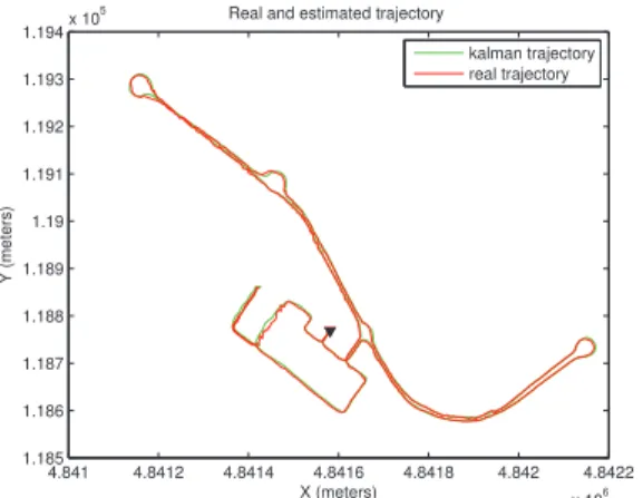
2) Trajectory estimation by Kalman filter : Figure 8 shows the estimated trajectory by kalman filter.
Figure 9 shows the variation of the positioning error during simulation time. We obtained a mean squared error equals
to : EQM = 4.6975 m. We can conclude that the estimated
0 500 1000 1500 2000 2500 3000 0
50 100 150
Diff. between theoretical and estimated 2D positions (m)
Time (s) Mean value = 5.5928
Fig. 7: Positioning error vs time for scenario 1 using the least squares method. 4.841 4.8412 4.8414 4.8416 4.8418 4.842 4.8422 x 10⁶ 1.185 1.186 1.187 1.188 1.189 1.19 1.191 1.192 1.193 1.194x 10 5 X (meters) Y (meters)
Real and estimated trajectory
kalman trajectory real trajectory
Fig. 8: Estimated trajectory by Kalman filter for scenario 1.
m. So, the Kalman filter provides a good trajectory estimation.
0 500 1000 1500 2000 2500 3000 3500 0 5 10 15 20 25 30
Diff. between theoretical and estimated 2D positions (m)
Time (s) Mean value = 4.6975
Fig. 9: Positioning error vs time for scenario 1 using kalman filter.
3) Comparison : In order to compare the Kalman filter and the Least Square method, we computed the squared error of
position averaged over two trajectory (cf. table II).
From table II, we noted an improvement of positioning about
Mean squared error of posi-tion (meter)
Squared errors of po-sition averaged over two trajectory (meter) Trajectory 1(cf. figure5a) Trajectory 2(cf. figure5b) Least Square method 5.5928 6.6591 6.12595 Kalman filter 4.6975 6.2373 5.4674
TABLE I: Squared errors of position averaged over two trajectory.
66 centimeter with the Kalman filter compared to the Least Square method.
B. Scenario 2:
In this scenario we used the same data of trajectory 1 (cf. figure 5a) used in scenario 1, except that between period of 100 to 200 seconds, we created disturbances in the signals coming from two satellites, in order to simulate that the signals have been under reflections before being received by the receiver. This disturbance is created by adding a delay of 120 to 200 meters at the pseudorange measurements provided by the receiver (we remind that the reflected signals take more time to reach the receiver than the direct signal, so an additional distance will be added to the pseudorange measurements).
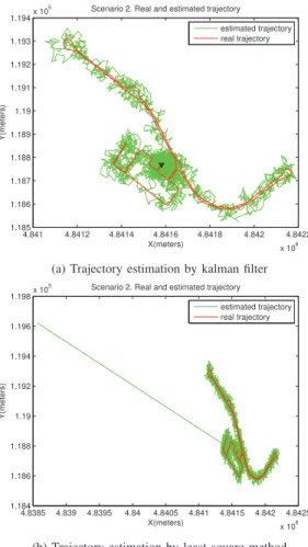
From the simulation results (cf. figures 10 and 11), we note that the estimated trajectory is shifted an average to the real trajectory by more than 30 meter. We can justify this important error that in constrained environments, the assumption made by the classical estimation methods (the observation noises are Gaussian) becomes not valid, because reflected signals add an additional error on pseudorange estimation, and several studies in literature have shown that the pseudorange error distribution becomes non-Gaussian [15] [16].
We can conclude, that in degraded environments, the classical positioning algorithms used in GNSS receiver show an important positioning errors because their measurement noise model is unsuitable.
VI. RECOMMANDATIONS
For adapting the measuremennt noise model of least square method and the kalman filter method in constrained environ-ment, we will propose an approach to model the multipath errors. The approach aims firstly to propose a technique to compute the multipath errors in real environment, secondly, in order to propose a statistical model and to search the distribution law of computed multipath errors, we propose to plot the probability density functions for some satellites in
4.841 4.8412 4.8414 4.8416 4.8418 4.842 4.8422 x 10⁶ 1.185 1.186 1.187 1.188 1.189 1.19 1.191 1.192 1.193 1.194x 10 5 X(meters) Y(meters)
Scenario 2. Real and estimated trajectory estimated trajectory real trajectory
(a) Trajectory estimation by kalman filter
4.8385 4.839 4.8395 4.84 4.8405 4.841 4.8415 4.842 4.8425 x 10⁶ 1.184 1.186 1.188 1.19 1.192 1.194 1.196 1.198x 10 5 X(meters) Y(meters)
Scenario 2. Real and estimated trajectory estimated trajectory real trajectory
(b) Trajectory estimation by least square method
Fig. 10: Biased trajectory estimation by Kalman filter and Least Square method for scenario 2.
indirect visibility and to see their behavior. We can also test the adequacy of computed multipath errors with the most common laws that describe the noise output of a telecommunications transmission chain and that modelize the signals delay, such as Normal and Rayleigh laws, using for example a visual validation with the Q-Q Plot Diagram.
Using the measurement model previously expressed (cf. equa-tion (1)), the pseudorange error is expressed as follows :
εst = ms t+ wt+ δts+ Its+ T s t + eph s t
We consider that δts, Its, ephst and Tts are modeled and
corrected, and the receiver noise wt is a Gaussian white
noise. Thus, According to signal reception state, ms
t can be
modeled in two different ways (cf. table II). If the signal
Signal receiving state ms
t
Direct(Line-of-sight reception) ms
t= 0
Reflexive (Multipath interference and NLOS reception) ms
t≁ N (µ, σ)
TABLE II: Modeling multipath errors according to signal reception conditions
propagation is on line of sight (direct), ms
t is null. In the
opposite case (Multipath interference and NLOS reception),
0 500 1000 1500 2000 2500 3000 3500 0 20 40 60 80 100 120
Scenario 2. Diff. between theoretical and estimated 2D positions(m)
Time(s) Mean value = 31.4845
(a) Positioning error vs time using Kalman filter
0 500 1000 1500 2000 2500 3000 0 10 20 30 40 50 60 70 80 90 100
Scenario 2. Diff. between theoretical and estimated 2D positions(m)
Time(s) Mean value = 32.9253
(b) Positioning error vs time using Least Square method
Fig. 11: Positioning error vs time for scenario 2.
ms
t is not null and cannot be modeled by a gaussian noise.
Therefore, a model for multipath errors must be defined. Our approach aims to compute the residues of pseudorange which exhibit in our case the multipath errors. This residue will be computed by subtracting pseudorange, real geometric distance, different errors affecting signal during its propagation and the receiver noise (cf. equation 4 which illustrates the calculation of multipath error for satellite m at time t).
ms
t = ρst− [dst+ c ∗ δts+ Its+ Tts+ wt+ ephst] + X(4) (4)
Where :
• dst, δts, Its, Tts, ephst and wt are already defined in
equa-tion 1.
• ρst : Is the pseudo range measurement obtained by
mul-tiplying signal travel time by the speed of light.
• X(4) : Is the fourth element of state vector presented in
equation (2), which equals to c∗ δtu.
To search the probability distribution of multipath errors, we
propose to compute mst for a vehicle moving in urban areas.
VII. CONCLUSION ANDFUTURE WORK
In this paper, we gave a general presentation about GNSS systems and the major problems that disrupt the positioning
in urban areas.
Therefore, the performance of classical estimation methods used in GNSS receiver is analyzed in terms of mean squared error (MSE). Though the kalman filter estimation shows the best positioning accuracy in a good environment (Line-of-sight propagation), the use of classical filtering methods remain limited in constrained environments, because, the assumption made by these methods becomes not valid.
In order to improve positioning in constrained environments, our future works will be focused on applying the technique proposed in this article to compute the multipath errors in a realistic scenario, in order to search their statistical model, and to adapt the measurement noise model of the kalman filter and the least square method with the multipath error model found.
ACKNOWLEDGMENT
This work was financially supported by the National Center of Scientific and Technical Research (CNRST), Morocco.
REFERENCES
[1] P Paimblanc, W Chauvet, D Bonacci, T Sadiki, and F Castani´e, “Improved positioning using gsm and gnss tight hybridization,” in
Proc. of the European Navigation Conf. on Global Navigation Satellite Systems (ENC–GNSS08), 2008.
[2] Safaa Dawoud, “Gnss principles and comparison,” Potsdam University. [3] Lindsay Kleeman, “Understanding and applying kalman filtering,” in
Proceedings of the Second Workshop on Perceptive Systems, Curtin University of Technology, Perth Western Australia (25-26 January 1996), 1996.
[4] Paul D Groves, Principles of GNSS, inertial, and multisensor integrated
navigation systems, Artech house, 2013.
[5] Bernhard Hofmann-Wellenhof, Herbert Lichtenegger, and Elmar Wasle,
GNSS–global navigation satellite systems: GPS, GLONASS, Galileo, and more, Springer Science & Business Media, 2007.
[6] Charles Jeffrey, “An introduction to gnss gps, glonass, galileo and other global navigation satellite systems. edn,” NovAtel Inc, 2010. [7] Kai Borre, Dennis M Akos, Nicolaj Bertelsen, Peter Rinder, and
Søren Holdt Jensen, A software-defined GPS and Galileo receiver: a
single-frequency approach, Springer Science & Business Media, 2007. [8] Phillip W Ward, John W Betz, and Christopher J Hegarty, “Satellite signal acquisition, tracking, and data demodulation,” Understanding GPS principles and applications, vol. 5, pp. 174–175, 2006.
[9] Steven J Miller, “The method of least squares,” Mathematics Department
Brown University, pp. 1–7, 2006.
[10] Paul D Groves, Ziyi Jiang, Morten Rudi, and Philip Strode, “A portfolio approach to nlos and multipath mitigation in dense urban areas,” 2013. [11] Lei Wang, Paul D Groves, and Marek K Ziebart, “Multi-constellation gnss performance evaluation for urban canyons using large virtual reality city models,” Journal of Navigation, vol. 65, no. 03, pp. 459–476, 2012. [12] PD Groves, “Gnss solutions: Multipath vs. nlos signals. how does non-line-of-sight reception differ from multipath interference,” Inside GNSS
Magazine, vol. 8, no. 6, pp. 40–42, 2013.
[13] Shodai Kato, Mitsunori Kitamura, Taro Suzuki, and Yoshiharu Amano, “Nlos satellite detection using a fish-eye camera for improving gnss po-sitioning accuracy in urban area,” Journal of Robotics and Mechatronics, pp. 31–39, 2016.
[14] Sven Bauer, Robin Streiter, and Gerd Wanielik, “Non-line-of-sight miti-gation for reliable urban gnss vehicle localization using a particle filter,” in Information Fusion (Fusion), 2015 18th International Conference on. IEEE, 2015, pp. 1664–1671.
[15] Juliette Marais and Baptiste Godefroy, “Analysis and optimal use of gnss pseudo-range delays in urban canyons,” in Computational Engineering
in Systems Applications, IMACS Multiconference on. IEEE, 2006, vol. 1, pp. 31–36.
[16] N Viandier, DF Nahimana, J Marais, and E Duflos, “Gnss performance enhancement in urban environment based on pseudo-range error model,” in Position, Location and Navigation Symposium, 2008 IEEE/ION. IEEE, 2008, pp. 377–382.