Evidence for differentiation of the most primitive small bodies

(1)

HAL Id: insu-03184663

https://hal-insu.archives-ouvertes.fr/insu-03184663

Submitted on 29 Mar 2021

HAL is a multi-disciplinary open access

archive for the deposit and dissemination of

sci-entific research documents, whether they are

pub-lished or not. The documents may come from

teaching and research institutions in France or

abroad, or from public or private research centers.

L’archive ouverte pluridisciplinaire HAL, est

destinée au dépôt et à la diffusion de documents

scientifiques de niveau recherche, publiés ou non,

émanant des établissements d’enseignement et de

recherche français ou étrangers, des laboratoires

publics ou privés.

bodies

Benoit Carry, P. Vernazza, F. Vachier, M. Neveu, J. Berthier, J. Hanuš, M.

Ferrais, Laurent Jorda, M. Marsset, M. Viikinkoski, et al.

To cite this version:

Benoit Carry, P. Vernazza, F. Vachier, M. Neveu, J. Berthier, et al.. Evidence for differentiation of

the most primitive small bodies. Astronomy and Astrophysics - A&A, EDP Sciences, 2021, (in press).

�insu-03184663�

(2)

March 12, 2021

Evidence for differentiation of the most primitive small bodies

?

,

??

B. Carry

1

, P. Vernazza

2

, F. Vachier

3

, M. Neveu

4,5

, J. Berthier

3

, J. Hanuš

6

, M. Ferrais

2,7

, L. Jorda

2

, M. Marsset

8

,

M. Viikinkoski

9

, P. Bartczak

10

, R. Behrend

11

, Z. Benkhaldoun

12

, M. Birlan

3,13

, J. Castillo-Rogez

14

, F. Cipriani

15

,

F. Colas

3

, A. Drouard

2

, G. P. Dudzi´nski

10

, J. Desmars

3,16

, C. Dumas

17

, J. ˇ

Durech

6

, R. Fetick

2

, T. Fusco

2

, J. Grice

1,18

,

E. Jehin

7

, M. Kaasalainen

9,???

, A. Kryszczynska

10

, P. Lamy

19

, F. Marchis

20

, A. Marciniak

10

, T. Michalowski

10

,

P. Michel

1

, M. Pajuelo

3,21

, E. Podlewska-Gaca

10,22

, N. Rambaux

3

, T. Santana-Ros

23,24

, A. Storrs

25

, P. Tanga

1

,

A. Vigan

2

, B. Warner

26

, M. Wieczorek

1

, O. Witasse

15

, and B. Yang

27 (Affiliations can be found after the references)

Received September 15, 1996; accepted March 16, 1997

ABSTRACT

Context.Dynamical models of Solar System evolution have suggested that the so-called P- and D-type volatile-rich asteroids formed in the outer Solar System beyond Neptune’s orbit and may be genetically related to the Jupiter Trojans, the comets and small Kuiper-belt objects (KBOs). Indeed, the spectral properties of P/D-type asteroids resemble that of anhydrous cometary dust.

Aims.We aim at gaining insights into the above classes of bodies by characterizing the internal structure of a large P/D-type asteroid.

Methods.We report high-angular-resolution imaging observations of P-type asteroid (87) Sylvia with VLT/SPHERE. These images were used to

reconstruct the 3D shape of Sylvia. Our images together with those obtained in the past with large ground-based telescopes were used to study the dynamics of its two satellites. We also model Sylvia’s thermal evolution.

Results. The shape of Sylvia appears flattened and elongated (a/b∼1.45 ; a/c∼1.84). We derive a volume-equivalent diameter of 271 ± 5 km, and a low density of 1378 ± 45 kg·m−3_{. The two satellites orbit Sylvia on circular, equatorial orbits. The oblateness of Sylvia should imply} a detectable nodal precession which contrasts with the fully-Keplerian dynamics of its two satellites. This reveals an inhomogeneous internal structure, suggesting that Sylvia is differentiated.

Conclusions.Sylvia’s low density and differentiated interior can be explained by partial melting and mass redistribution through water percolation.

The outer shell would be composed of material similar to interplanetary dust particles (IDPs) and the core similar to aqueously altered IDPs or carbonaceous chondrite meteorites such as the Tagish Lake meteorite. Numerical simulations of the thermal evolution of Sylvia show that for a body of such size, partial melting was unavoidable due to the decay of long-lived radionuclides. In addition, we show that bodies as small as 130–150 km in diameter should have followed a similar thermal evolution, while smaller objects, such as comets and the KBO Arrokoth, must have remained pristine, in agreement with in situ observations of these bodies. NASA Lucy mission target (617) Patroclus (diameter ≈140 km) may, however, be differentiated.

Key words. Minor planets, asteroids: individual: Sylvia; Kuiper belt: general

1. Introduction

The Cybele region, at the outer rim of the asteroid belt (3.27–3.7 au), is essentially populated by P- and D-type asteroids and to a lesser extent by C-type bodies (DeMeo & Carry,2013,2014). P- and D-type asteroids are thought to have formed in the outer Solar System (beyond 10 au), among the progenitors of the cur-rent Kuiper Belt, and to have been implanted in the inner So-lar System (asteroid belt, Lagrangian Points of Jupiter) follow-ing giant planet migrations (see Levison et al., 2009; DeMeo

et al.,2014; Vokrouhlický et al.,2016). This implies that the

P/D-type main belt asteroids and the Jupiter Trojans could be compositionally related to outer small bodies such as Centaurs, short-period comets, and small (D≤300km) Kuiper Belt Objects (KBOs). This dynamical scenario is currently supported by the

?

Based on observations made with ESO Telescopes at the La Silla

Paranal Observatory under program073.C-0851(PI Merline),

073.C-0062(PI Marchis),085.C-0480(PI Nitschelm),088.C-0528(PI Rojo),

199.C-0074(PI Vernazza).

?? _{The reduced and deconvolved SPHERE images are available}

at the CDS via anonymous ftp to http://cdsarc.u-strasbg.

fr/ or via http://cdsarc.u-strasbg.fr/viz-bin/qcat?J/A+

A/xxx/Axxx

??? _Deceased

similarity in size distributions between the Jupiter Trojans and small KBOs (Fraser et al.,2014) as well as the similarity in terms of spectral properties between P/D-type main belt asteroids, the Trojans of Jupiter and comets (Vernazza et al.,2015;Vernazza & Beck,2016).

Overall, the outer Solar system is of tremendous interest, as it is recognized as the least processed since the dawn of the Solar System and thus the closest to the primordial materials from which the Solar System formed (e.g., McKinnon et al.,

2020). This is currently supported by the analysis of the spec-tral properties of P/D-type main belt asteroids, Jupiter Trojans, and comets that reveal a surface composition compatible with that of anhydrous chondritic porous interplanetary dust particles (CP IDP, seeVernazza et al.,2015). The CP IDPs are currently seen among the available extra-terrestrial materials as the clos-est to the starting ones (Bradley,1999). In particular, based on its albedo and visible, near- and mid-infrared spectrum, it is now well established (seeVernazza et al.,2013) that the aqueously altered Tagish Lake meteorite cannot be representative of the surface composition of D-type asteroids nor that of most P-type asteroids as suggested earlier (Hiroi et al.,2001). As such, CP IDPs are currently the most likely analogs of the refractory ma-terials present at the surface of P/D type asteroids.

(3)

There are only four known large (diameter ≥100 km) P/D-type asteroids with satellites: (87) Sylvia, (107) Camilla, (617) Patroclus, and (624) Hektor, with reported densi-ties of 1,400 ± 200 kg·m−3 (e.g., Berthier et al., 2014), 1,280 ± 130 kg·m−3 ₍_Pajuelo _et _al._, ₂₀₁₈_), ₈₀₀+200

−100 to

1080 ± 330 kg·m−3 ₍_{Marchis et al.}_, ₂₀₀₆_; _{Mueller et al.}_,

2010), and 1,000 ± 300 kg·m−3 (Marchis et al., 2014) respec-tively. Patroclus is a double asteroid with nearly equally-sized 150 km-100 km components (e.g., Buie et al., 2015; Hanuš

et al., 2017; Berthier et al., 2020) and is therefore atypical

among asteroids but further strengthens the common origin of P/D asteroids and small KBOs (Nesvorný et al.,2018), many of which likely formed as binaries (Fraser et al.,2017;Nesvorný

et al., 2019; Robinson et al., 2020). Both Camilla and Sylvia

are among the largest asteroids, with diameters above 250 and 280 km respectively (Carry,2012). Their low density implies a bulk composition that cannot consist only of refractory materials but that must also comprise a large amount of volatiles (Pajuelo

et al.,2018).

With an estimated diameter of nearly 280 km (Carry,2012, and reference therein), (87) Sylvia is the largest body in the Cy-bele region and more generally the largest P/D-type asteroid in the inner (≤5.5 au) Solar System. Its surface composition is fully consistent with that of anhydrous chondritic porous IDPs (

Ver-nazza et al.,2015;Usui et al.,2019). Furthermore, it is the first

asteroid around which two satellites were discovered (Marchis

et al.,2005). Because of its rather large angular size at

oppo-sition (≈0.1400) and its two moons, Sylvia is an ideal target for high angular-resolution adaptive-optics observations as these al-low an accurate characterization of its 3D shape and of the mass of the system, hence of its bulk density. Furthermore, the two moons allow probing the internal structure and in particular the harmonics of the gravity field (at least the lowest-order gravi-tational moment, the quadrupole J2). This information, in turn,

probes the distribution of material inside Sylvia, i.e., whether its interior is homogeneous or differentiated.

Several authors have studied Sylvia’s dynamical system

(Marchis et al.,2005;Winter et al.,2009;Frouard & Compère,

2012; Fang et al.,2012;Beauvalet & Marchis,2014; Berthier

et al.,2014;Drummond et al.,2016). While these studies agreed

on the mass of Sylvia and its low density (around 1,300 kg·m−3), there is no consensus regarding its gravitational potential (of which only the quadrupole J2 has been studied, Table 1). The

latter is, however, a direct consequence of the internal structure of Sylvia.

To constrain the bulk density of Sylvia and its internal struc-ture, we observed it as part of our imaging survey of D≥100 km main-belt asteroids (ID 199.C-0074, PI P. Vernazza, see

Ver-nazza et al.,2018,2020;Viikinkoski et al.,2018;Fétick et al.,

2019; Carry et al., 2019; Hanuš et al., 2019, 2020; Marsset

et al.,2020;Yang et al.,2020;Ferrais et al.,2020). We imaged

Sylvia over two apparitions, separated by a year, throughout its rotation at high angular resolution with the SPHERE extreme adaptive-optics (AO) IRDIS and ZIMPOL cameras (Thalmann

et al.,2008;Dohlen et al.,2008;Beuzit et al.,2019) mounted

on the European Southern Observatory (ESO) Very Large Tele-scope (VLT). Beyond contributing to our understanding of the formation and evolution of the Solar System’s most primitive bodies, the present study provides the context for the future in-situ exploration of primitive P/D-type bodies by NASA’s Lucy mission to the Jupiter Trojans.

2. Observations and data reduction

2.1. High-angular-resolution imaging

The data used in the present study to extract the position of the moons comprises all the high angular resolution images of Sylvia taken with the Hubble Space Telescope (HST) and ground-based telescopes equipped with adaptive-optics (AO) cameras: Gemini North, ESO VLT, W. M. Keck, and SOR

(Drummond et al., 2016). The data span 51 different epochs,

with multiple images each, over 17 years from February 2001 to November 2018. For the reconstruction of Sylvia’s 3D shape, however, only the images with the highest resolution were used, i.e., those acquired with VLT/SPHERE/ZIMPOL (Section 3).

The images from the HST were obtained with the second Wide Field and Planetary Camera (WFPC2, Holtzman et al.,

1995). The images from the VLT were acquired with both the first generation instrument NACO (NAOS-CONICA, Lenzen

et al., 2003; Rousset et al., 2003) and SPHERE

(Spectro-Polarimetric High-contrast Exoplanet REsearch, Fusco et al.,

2006;Beuzit et al.,2019), the second generation extreme-AO

in-strument designed for exoplanet detection and characterization. The images acquired with SPHERE were taken with both the IRDIS (InfraRed Dual-band Imager and Spectrograph, Dohlen

et al.,2008) and ZIMPOL (Zurich Imaging Polarimeter,

Thal-mann et al., 2008) sub-systems. Images taken at the Gemini

North used the NIRI camera (Near InfraRed Imager, Hodapp

et al., 2003), fed by the ALTAIR AO system (Herriot et al.,

2000). Finally, observations at Keck were acquired with the guiding camera of NIRSPEC in 2001 (McLean et al.,1998) and NIRC2 (Near-InfraRed Camera 2, van Dam et al.,2004;

Wiz-inowich et al.,2000) later on.

To reduce the AO-imaging data, a standard data process-ing protocol (sky subtraction, bad-pixel identification and cor-rection, and flat-field correction) was followed using in-house routines developed in Interactive Data Language (IDL) (see

Carry et al.,2008). The images were then deconvolved with the

Mistral algorithm (Fusco,2000; Mugnier et al.,2004) to re-store their optimal angular resolution (seeFétick et al.,2019, for details). Separately, the reduced images were processed to subtract the bright halo surrounding Sylvia to enhance the de-tectability of the satellites (seePajuelo et al.,2018;Carry et al.,

2019, for details).

2.2. Optical lightcurves

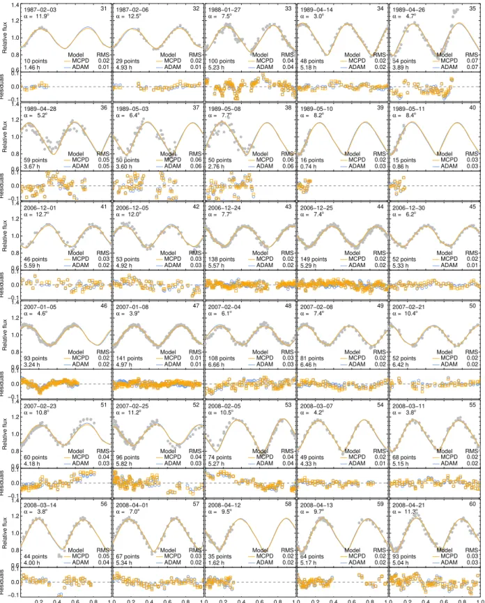
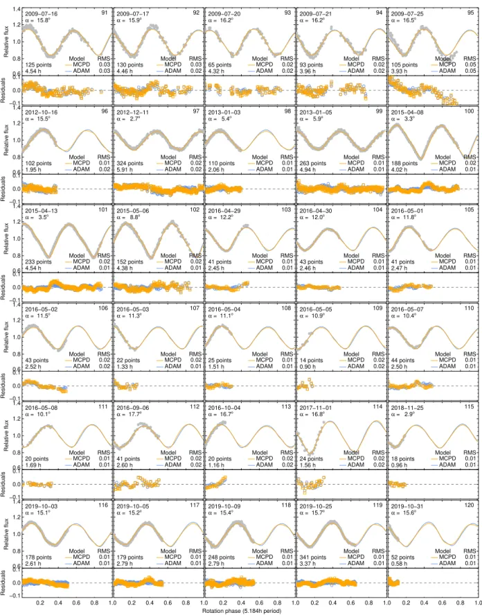
We used the 40 lightcurves from Kaasalainen et al.(2002) to create a convex 3-D shape model of Sylvia1, compiled from the Uppsala Asteroid Photometric Catalog2₍_{Lagerkvist &}

Magnus-son,2011). We also compiled 11 lightcurves acquired by ama-teur astronomers within the Courbes de rotation d’astéroïdes et de comètes database (CdR3).

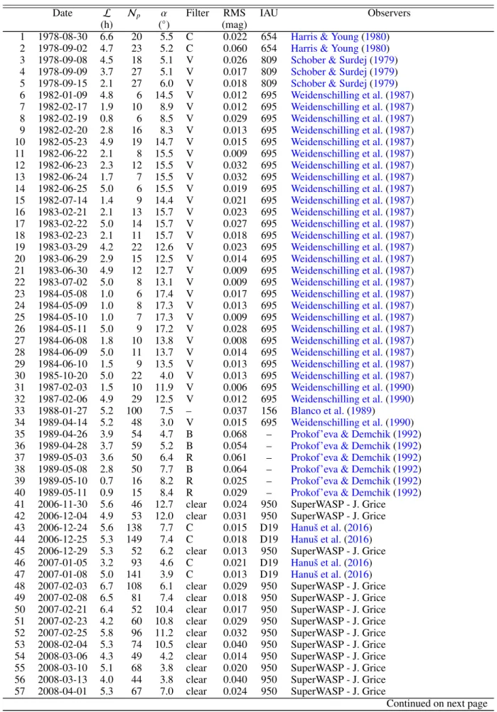
In addition to these data, we acquired 12 lightcurves using the 60 cm André Peyrot telescope mounted at Les Makes obser-vatory on La Réunion Island, operated as a partnership among Les Makes Observatory and the IMCCE, Paris Observatory, and 7 lightcurves with the 60 cm TRAPPIST telescopes located at La Silla Observatory in Chile and the Oukaïmeden observatory in Morocco (Jehin et al.,2011). Finally, we extracted 51 lightcurves from the data archive of the SuperWASP survey (Pollacco et al.,

1 _{Available on DAMIT (}_{Durech et al.}_ˇ _,₂₀₁₀_): https://astro.troja.mff.cuni.cz/projects/damit/

2 _{http://asteroid.astro.helsinki.fi/apc/asteroids/}

(4)

Satellite Nobs Mass Density J2 Reference

(×1019_kg) _(kg·m−3₎

Romulus 24 1.48 ± 0.01 1200 ± 100 0.17 ± 0.05 Marchis et al.(2005) Remus 12 1.47 ± 0.01 1200 ± 100 0.18 ± 0.01 Marchis et al.(2005) Both 45+20 1.484 ± 0.015 1290 ± 390 0.099 59 ± 0.000 84 Fang et al.(2012)

Both 51+17 1.476 ± 0.006 1200 ± 100 0.000 002 ± 0.000 300 Beauvalet & Marchis(2014) Romulus 65 1.476 ± 0.166 1380 ± 150 0 ± 0.01 Berthier et al.(2014) Remus 25 1.380 ± 0.223 1290 ± 200 0 ± 0.024 Berthier et al.(2014) Romulus 76 1.470 ± 0.008 1350 ± 40 – Drummond et al.(2016) Both 143+68 1.44 ± 0.01 1378 ± 45 0 ± 0.01 Present study

Table 1: Mass, density, and quadrupole J2 of Sylvia, derived using either Romulus, Remus, or both satellite, from the literature

compared with the present study.

2006) for the period 2006-2009 (Parley et al.,2005;Grice et al.,

2017). In summary, a total of 121 lightcurves observed between 1978 and 2017 (Table A.1) were used in this work and are pre-sented inFigure A.1.

2.3. Stellar occultations

Nine stellar occultations by Sylvia have been recorded since 1984, mostly by amateur astronomers during the last decade (see

Mousis et al.,2014;Dunham et al.,2016;Herald et al.,2020).

We converted the timings of disappearance and reappearance of the occulted stars4_{into segments (called chords) on the plane of}

the sky, using the location of the observers on Earth and the ap-parent motion of Sylvia following the recipes listed inBerthier

(1999). Only five stellar occultations had multiple chords that could be used to constrain the size and apparent shape of Sylvia

(Figure B.1). For the January 2013 and October 2019

occulta-tions, several observers reported secondary events due to the oc-cultation of the stars by either Romulus or Remus (Berthier et al.,

2014;Vachier et al.,2019). We thus used the relative positions

between Sylvia and its satellites at the time of the occultations to constrain their mutual orbits. We list the observers of the occul-tations inTable B.1.

3. Sylvia’s 3D shape

We fed the All-Data Asteroid Modeling (ADAM) algorithm with all SPHERE/ZIMPOL images, lightcurves, and stellar occulta-tions to determine the spin and 3D shape of Sylvia (Viikinkoski

et al., 2015a). Optical lightcurves are often required for ADAM

to constrain the regions not imaged and to stabilize the shape optimization. The procedure is similar to that published in our previous studies with SPHERE, and we refer to these for more details (e.g.,Viikinkoski et al.,2015b;Marsset et al.,2017;

Ver-nazza et al.,2018). We used the sidereal rotation period and the

spin-axis coordinates of Sylvia from the literature (Kaasalainen

et al.,2002;Hanuš et al.,2013,2017) as input values to ADAM.

We further model the shape by using the Multi-resolution PhotoClinometry by Deformation (MPCD) method (Jorda et al.,

2016), following the procedure of our previous works (e.g.,

Fer-rais et al.,2020). MPCD gradually deforms the vertices of a

previ-ous mesh (here ADAM model) to minimize the difference between the observed images and synthetic images of the model (Jorda

et al.,2010). Both models only present marginal differences (

Ta-ble 2), and in what follows, we report on the MPCD model.

4 _{compiled by}_{Dunham et al.}₍₂₀₁₇_{) and publicly available on the} Plan-etary Data System (PDS):http://sbn.psi.edu/pds/resource/occ.html

The derived shape is in essence similar to that based on lower angular resolution images (Berthier et al.,2014; Hanuš et al.,

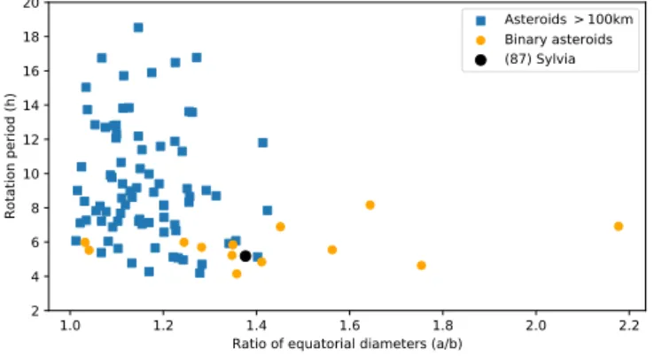
2017). A striking feature of Sylvia is its remarkable elongated shape (Table 2,Figure 2). To put its peculiar shape into con-text, we measured the tri-axial diameters of 103 asteroids larger than 100 km from their shape models5and compiled their rota-tion periods from the Planetary Data System (Harris et al.,2017). Sylvia appears to be more elongated and to spin faster than most asteroids larger than 100 km (Figure 2). In particular, the popu-lation of asteroids with satellites stands out from the popupopu-lation of singletons, with a median ratio of equatorial diameters a/b of 1.37 (vs 1.16 for the background) and a median rotation pe-riod of 5.5 h (vs 7.9 h for the background). We compared the a/b ratio and rotation period distributions of asteroids with and with-out satellites using the Kolmogorov-Smirnov test. The p-values for both are 5 · 10−4and 7 · 10−5respectively. We thus conclude that the distributions are different above the 99.5% confidence level. While asteroids with a diameter smaller than about 15 km are subject to YORP spin-up and surface re-arrangment (Walsh

et al.,2008; Vokrouhlický et al.,2015), Sylvia is too large to

have been affected. The origin of this difference is thus unclear. It may result from the impact at the origin of the satellite for-mation (Margot et al.,2015), or alternatively, satellites may be more stable around elongated bodies (seeWinter et al.,2009).

4. Dynamics of the system

The two satellites orbit Sylvia on equatorial, circular, and pro-grade orbits (Table 3). The root mean square (RMS) residual between the observations and the computed positions is only 9.3 mas, that is within the pixel size of most observations. The positive occultations by both satellites in October 2019 provide a practical estimate of the reliability of the orbital solution, as the two satellites were detected at only 5 mas from the positions we predicted (Vachier et al.,2019). It also highlights the impor-tance of accurate ephemerides to prepare the observation of the occultation by placing observers on the path of the satellites.

The mass of Sylvia is constrained with an uncertainty of less than 1% : (1.44 ± 0.01) × 1019_{kg, thanks to the long baseline}

of observations. Combined with our volume-equivalent diam-eter estimate (271 ± 5 km, see above), the density of Sylvia is found to be 1378 ± 45 kg·m−3, reminiscent of that of other large asteroids with a surface composition consistent with that of IDPs (C/P/D types, seeCarry,2012;Vernazza et al.,2015). We present

inFigure 3all the possible bulk compositions of Sylvia,

consid-5 _{Retrieved from DAMIT (}_{Durech et al.}_ˇ _,₂₀₁₀_): https://astro.troja.mff.cuni.cz/projects/damit/

(5)

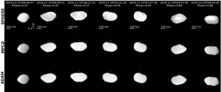
Fig. 1: Comparison of the SPHERE image (top row) with the MPCD (middle) and ADAM (bottom) models.

Table 2: Spin solution (coordinates in ecliptic and equatorial J2000 reference frames) and shape model parameters (the overall shape is reported as the a > b > c diameters of a triaxial ellipsoid fit to the shape model). All uncertainties are reported at 1 σ.

Parameter MPCD ADAM Unc. Unit

Sidereal period Ps 5.183 641 3.9 ·10−5 hour

Longitude λ 75.3 5 deg.

Latitude β +64.2 5 deg.

Right Ascension α 14.3 5 deg.

Declination δ +83.5 5 deg. Ref. epoch T0 2443750.000 Diameter D 271 274 5 km Volume V 1.05 ·107 _{1.08 ·10}7 _{2 ·10}5 _km3 Diameter a a 363 374 5 km Diameter b b 249 248 5 km Diameter c c 191 194 5 km Axes ratio a/b 1.46 1.51 0.03 Axes ratio b/c 1.30 1.28 0.04 Axes ratio a/c 1.90 1.93 0.05

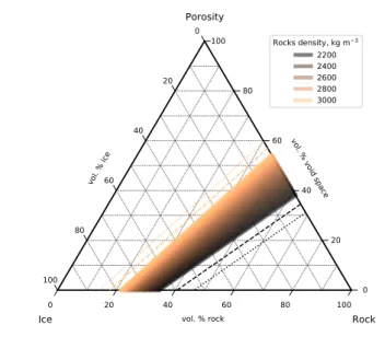
ering a mixture of rocks and ices, with voids. We use a range of density from 2200 to 3000 kg·m−3for the rock phase (from rocks with organics to the density of the silicate phase reported by the Stardust mission,Brownlee et al.,2006). The density of Sylvia implies the presence of both ices and macroporosity in its interior.

We estimate the masses of Romulus and Remus at (1.4 ± 1.2) × 1015_{kg and (7.8 ± 7.3) × 10}14_{kg (i.e., e}_ffectively

upper limits), very close to the masses reported by Fang et al.

(2012). Assuming a similar albedo for Sylvia and its two moons, their magnitude differences with Sylvia (Table 3) imply diame-ters of 15+10₋₆ km and 10+17₋₆ km for Romulus and Remus (consis-tent with occultation chords,Berthier et al.,2014), hence densi-ties of 790 ± 680 and 1480 ± 1400 kg·m−3. The density of both satellites is loosely constrained and similar to that of Sylvia.

Finally, we note that the best orbital solutions are obtained for the smallest quadrupole J2(Figure 4), tending toward J2=0

(i.e., fully Keplerian orbits over the 19 years baseline). Although there are orbits fitting the data within 1 σ of the observations, their residuals are systematically larger.

5. Implication for the internal structure

Under the assumption of a homogeneous density in the interior, the shape of Sylvia implies a J2of 0.082 ± 0.005 (computed with

SHTOOLS6, seeWieczorek & Meschede,2018). This values con-trasts with the null J2determined dynamically (Section 4). This

discrepancy reveals an inhomogeneous density distribution in-side Sylvia and hints at a more spherical mass concentration than suggested by Sylvia’s oblate and elongated 3D shape. This im-plies a denser, more spherical core, surrounded by a less dense envelope. Based on similar considerations, similar internal struc-tures have recently been proposed for other large P-types such as the Cybele (107) Camilla (Pajuelo et al.,2018) and the Jupiter Trojan (624) Hektor (Marchis et al.,2014).

This differentiated structure is at odds with the IDP-like spectral properties, evidence for an absence of both thermal metamorphism and aqueous alteration. This suggests that par-tial differentiation occurred, limited by the insufficient amount of heat generated by radionuclides which did not propagate to the

(6)

Table 3: Orbital elements of the satellites of Sylvia, expressed in EQJ2000, obtained with Genoid: orbital period P, semi-major axis a, eccentricity e, inclination i, longitude of the ascending nodeΩ, argument of pericenter ω, time of pericenter tp. The number of

observations and RMS between predicted and observed positions are also provided. Finally, we report the mass of Sylvia MSylvia,

the mass of Romulus MRomulus, the mass of Remus MRemus, their apparent magnitude difference ∆m with Sylvia, the ecliptic J2000

coordinates of the orbital pole (λp, βp), the equatorial J2000 coordinates of the orbital pole (αp, δp), and the orbital inclination (Λ)

with respect to the equator of Sylvia. Uncertainties are given at 3-σ.

Romulus Remus

Observing data set

Number of observations 130 66

Time span (days) 6050 5656

RMS (mas) 9.85 8.24

Orbital elements EQJ2000

P(day) 3.64126 ± 0.00005 1.35699 ± 0.00075 a(km) 1340.6 ± 1.2 694.2 ± 0.4 e 0.000 +0.009_−0.000 0.005 +0.031_−0.005 i(◦) 7.4 ± 1.6 8.7 ± 5.4 Ω (◦₎ _97.1 _{± 5.8} _100.8 _{± 20.6} ω (◦₎ _171.0 _{± 10.5} _262.2 _{± 25.9} tp(JD) 2455597.08689 ± 0.10085 2455594.89253 ± 0.10444 Physical parameters MSylvia(×1019kg) 1.440 ± 0.004 MRomulus(×1015kg) 1.4 ± 1.2 MRemus(×1014kg) 7.8 ± 7.3 ∆mRomulus 6.2 ± 1.1 ∆mRemus 7.1 ± 2.1 Derived parameters λp, βp(◦) 73,+65 ± 4, 1 70,+64 ± 11, 3 αp, δp(◦) 7,+83 ± 6, 2 11,+81 ± 21, 5 Λ (◦₎ ₅ _{± 1} ₆ _{± 4} DRomulus(km) 15.1 ± 1.1 D_Remus(km) 10.3 ± 2.1 1.0 1.2 1.4 1.6 1.8 2.0 2.2 Ratio of equatorial diameters (a/b)

2 4 6 8 10 12 14 16 18 20 Rotation period (h) Asteroids > 100km Binary asteroids (87) Sylvia

Fig. 2: Distribution of the ratio of equatorial diameters (a/b) and rotation period of 103 asteroids larger than 100 km in diameter. The difference between asteroids with and without satellites is striking.

surface. Such structures have indeed been suggested for the par-ent bodies of CV carbonaceous chondrites (Elkins-Tanton et al.,

2011), ordinary chondrites (Bryson et al.,2019), and mid-sized KBOs (Desch et al.,2009).

Building upon the work of Neveu & Vernazza(2019), we model the thermal and internal structure history of Sylvia. The evolution of internal temperatures and structure is computed

nu-merically using a one-dimensional code (Desch et al., 2009). Sylvia is assumed to be made of rock (idealizing a mixture of refractory materials such as silicates, metals, and organic mate-rial), water ice, and voids (the macroporosity). The mass is dis-tributed assuming spherical symmetry over 200 grid zones ini-tially evenly spaced in radius. The internal energy in each grid zone is computed from the initial temperature using equations of state for rock and ice. Material is never hot enough in our simu-lations for rock-metal differentiation, which is neglected. Initial radionuclide abundances are provided in Table 1 of Neveu &

Vernazza(2019). Simulations start once Sylvia is fully formed,

neglecting the progressive accretion of material over time. Be-cause of this and the near-absence of short-lived radionuclide heating given the assumed formation time, Sylvia’s simulated early evolution is cold. The implementation of instantaneous dif-ferentiation in the central regions that warm above 273 K rests on the assumption that sufficiently large rock grains settle via Stokes flow on timescales smaller than one time step.

Sylvia is assumed to accrete homogeneously at 60 K, 6 mil-lion years (My) after the formation of Ca-Al-rich inclusions (consistent with a surface without aqueous alteration; Neveu &

Vernazza,2019). It is the equilibrium temperature for an albedo

0.05 at a distance of 17-18 au (i.e., the postulated accretion dis-tance of KBOs, Morbidelli & Nesvorn`y, 2020) from the Sun with 70% of the present-day luminosity. The surface tempera-ture is instantaneously raised to 148 K (the present-day

(7)

equilib-0 20 40 60 80 100 100 80 60 40 20 0 0 20 40 60 80 100 vol. % ice vol. % rock

vol. % void space

Ice Rock Porosity Rocks density, kg m3 2200 2400 2600 2800 3000

Fig. 3: Bulk composition of Sylvia, assuming three end mem-bers: rocks, ices (density of 920 kg·m−3_{), and voids. The dashed}

and dotted lines represent the 1 and 2 σ boundaries.

0 0:02 0:04 0:06 0:08 0:10 J2 300 400 500 600 700 800 R es id u a ls (X 2) 1:426 1:428 1:430 1:432 1:434 1:436 1:438 1:440 1:442 M a ss o f S y lv ia (£ 1 0 1 9k g )

Fig. 4: Orbital residuals (χ2_{) as function of the dynamical}

quadrupole J2. The horizontal grey line corresponds to the χ2

providing a fit at 1 σ of the observations.

rium temperature) at the time of heliocentric migration. We test different timings, from a late planet migration (hundreds of My) such as the one described by the Nice model (Tsiganis et al.,

2005;Morbidelli et al.,2005;Gomes et al.,2005;Levison et al.,

2009) to an early dynamical instability occurring a few My after the dissipation of the gas disk (Nesvorný et al.,2018;Clement

et al.,2019), and find that the timing of implantation into the

as-teroid belt seldom affects its structure or peak temperature. In the results below, the time of migration is set to 6 My after formation (i.e., 12 My after Ca-Al-rich inclusions).

The thermal structure is determined by balancing conduc-tive heat transfer with primarily radiogenic heating by26_Al,40_K, 232_Th,235_{U, and}238_{U, using a finite-di}_{fference method and a}

50-yr time step, for 5 billion years (Gy). Thermal conductivities depend mainly on porosities (Figure 6), but also on composi-tion and temperature (Desch et al.,2009). Porosity is allowed

to compact at rates determined from material viscosities as de-scribed inNeveu & Rhoden (2017). Sylvia’s bulk density con-strains the void porosity and rock volume fractions to about 40– 55% and 20–35%, respectively, mainly depending on the rock density (Figure 3).

Convection is generally neglected as it is assumed that the postulated porous, rock-rich internal structure for Sylvia is not prone to fluid or ice advection. In the ice-rich case (Figure 5, right panel), solid-state convection is allowed to occur but does not, because the critical Rayleigh number is never exceeded. Al-though this was not simulated, in the percolation case below we expect convection to be possible in the central region rich in liq-uid water, until this region refreezes. In all simulations, volume changes due to water melting or freezing are neglected.

The viscosity of ice-rock mixtures, used to compute the Rayleigh number and pore compaction, is calculated following

Roberts(2015). Above 30 vol.% ice, it is equated to the viscosity

of ice. Below 30% ice volume fraction, as a first approximation, it is set to the geometric mean of the rock and ice viscosities at given grain size, stress (equated with hydrostatic pressure), and temperature.Roberts(2015) noted that this approximation tends to underestimate mixture viscosities relative to extrapolations of laboratory measurements. The ice and rock flow laws adopted in the model are the composite rheology ofGoldsby & Kohlstedt

(2001) and the dry diffusion creep flow law for olivine of

Kore-naga & Karato(2008), respectively.

The key factor governing thermal evolution in these simula-tions is porosityΦ, which decreases thermal conductivities k of rock-ice mixtures, of order 1 W m−1 _K−1 ₍_{Desch et al.}_,₂₀₀₉_,

and references therein), by up to two orders of magnitude. The adopted thermal conductivity-porosity relationship (Shoshany

et al.,2002) is derived from Monte-Carlo modeling of porous

cometary ice: k is decreased with increasingΦ via multiplica-tion by a factor (1 -Φ /0.7)nΦ+0.22_{. This relationship is shown in}

Figure 6. We adopt n=4.1 (grey curve) for the canonical

simu-lation with 52% porosity, following the discussion inShoshany

et al.(2002). We set n=3.5 (black curve) for the simulation with

60% porosity; choosing n=4.1 would result in more heating and compaction than shown inFigure 5. There is a wide spread in the Monte Carlo results ofShoshany et al.(2002) in howΦ af-fects k, with some of their models suggesting a lesser effect of porosity. Conversely, independent measurements of porous sil-ica aggregates (Krause et al.,2011) and extrapolated results from models of highly porous aggregates (Arakawa et al.,2017) both suggest similar or slightly higher decrease factors due to poros-ity (Figure 6) than the relationships we have assumed. Thus, the assumed relationships seem to adequately represent the state of understanding of how porosities of 50 to 60 vol.% decrease ther-mal conductivities.

Crucially, to be compatible with Sylvia’s observed anhy-drous surface and low J2despite an oblate shape, time-evolution

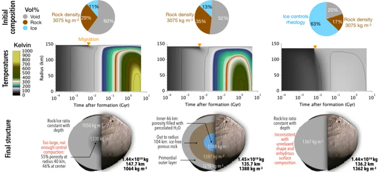
simulations with this model constrain the volume fraction of wa-ter to be low, less than 40 vol% relative to rock or 15 vol% overall. For higher volume fractions, ice grains tend to become adjoined and control the mechanical properties of the interior. In that case, the material viscosity is assumed equal to that of water ice (Goldsby & Kohlstedt,2001), and any void porosity rapidly decreases as the interior warms due to radiogenic heat-ing and porosity insulation. Instantaneous ice-rock di fferentia-tion happens first once the central (warmest) regions warm above 273 K. It then proceeds outward if the interior keeps warming. This yields a gravitationally unstable structure: the topmost un-differentiated layers are denser than underlying layers, which are poorer in rock. Once Sylvia is differentiated out to more than

(8)

Te m pe ra tu re s 11% 29% 60% Void Rock Ice 13% 35% 52% _63% 17% 20% Initial composition Vol% Rock density

3075 kg m-3 Rock density _{3075 kg m}-3 Rock density

3075 kg m-3 Ice controls rheology Kelvin Migration Fin al str uc tu

re porosity filled with Inner 46 km: percolated H2O Out to radius 104 km: ice-free porous rock Primordial outer layer 1788 kg m-3 1587 kg m-3 1218 kg m-3 Rock/ice ratio constant with depth

Too large, not enough central compaction: 55% porosity at radius 40 km, 46% at center Inconsistent with unrelaxed shape and anhydrous surface composition Rock/ice ratio constant with depth 1367 kg m-3 1050 kg m-3 1330 kg m-3 1.44×1019 _kg 147.7 km 1064 kg m-3 1.45×1019 _kg 135.7 km 1388 kg m-3 1.44×1019 _kg 136.2 km 1362 kg m-3

Fig. 5: Long-term evolution of the internal structure of Sylvia. The baseline scenario is presented in the central column, while the left and right columns present extreme cases in which the structure is dictated by rock-compaction and water ice rheology, respectively.

Fig. 6: Effect of porosity Φ on the thermal conductivity k. The or-ange and teal curves show relationships that were only validated in the regimes where the curves are solid. The orange curve is a thermal conductivity in W m−1_K−1_{(rather than a decrease}

fac-tor). Data points of a given color are from the same source as the fit curve of that color.

half its radius, differentiation is assumed to proceed by gravi-tational (Rayleigh-Taylor) instabilities: layers overturn if their viscosity is below a threshold that corresponds to T≈150 K (

Ru-bin et al.,2014). Since Sylvia’s post-migration surface

temper-ature is warmer, 148 K, differentiation out to the surface is es-sentially inevitable. This ought to result in evidence of surface water, either as ice or as mineral hydration, as observed on

aster-oids linked to carbonaceous chondrites (Rivkin & Emery,2010;

Campins et al.,2010). This is inconsistent with Sylvia’s

anhy-drous, IDP-like surface composition. Ice-rock differentiation can be prevented if ice dominates the volume fraction (Figure 5, right column), since in that case the combination of low rock (i.e., ra-dionuclide) content and low insulating void porosity results in a cold interior in which ice never melts. However, in such a homo-geneous interior, the mass distribution should result in a higher J2than observed given Sylvia’s oblate shape.

It follows that to retain a pristine anhydrous external enve-lope, Sylvia’s water volume fraction must be low (consistently with observations of the comet 67P nucleus by the Rosetta space-craft; Pätzold et al.,2019;Choukroun et al.,2020) so that inte-rior solids are less prone to deformation, inhibiting both porosity compaction and instability-driven differentiation. As a canonical case, we assume an interior comprised of 52 vol.% void porosity, 35% rock of density 3075 kg m−3_{, and 13% water (}_{Figure 5}_,

cen-tral column). The void porosity decreases the interior’s thermal conductivity by a factor of ≈15 relative to a compact rock-ice mixture. This favors accumulation of radiogenic heat, melting ice in the central regions after ≈0.15-0.2 Gy. At such low water volume fraction and high void porosity, it is sensible for liquid water to percolate downward in pores without significantly dis-turbing the remaining rock-void porosity structure, since rock grains already tend to be adjoined (see Fig. 3a,b of Neumann

et al.,2020, for a pictorial description). This would result in a

three-layer structure (Figure 5, bottom central panel): a central region where the porosity has been filled with percolated wa-ter, surrounded by a porous layer free of wawa-ter, and a primordial outer layer that remains too cold for ice to melt. Our thermal evolution simulations do not explicitly track percolation. The example interior structure ofFigure 5, bottom central panel is obtained by manually moving the mass of water that is liquid at 0.2 Gy to fill porosity at the center, and assuming that in the mid-dle layer, the empty volume left behind by the displaced water is compacted (so that the void porosity remains 52% in this layer). This compaction leads to a volume-averaged diameter decrease

(9)

from 283.4 km to 271.4 km, the observed value. The spherical central mass distribution in this three-layer model implies a J2

of 5 · 10−5_{only, consistent with the observed dynamics of both}

satellites.

Although this is not a unique solution, assuming lower rock densities (Figure 3) requires increasing the rock volume fraction at the expense of ice or void porosity so as to keep matching Sylvia’s bulk density. Neither the bulk ice volume fractions nor the bulk void porosity are likely to be much lower than assumed given the need to invoke the migration of melted ice, enabled by the insulating effect of porosity, to explain a more spherical mass distribution (low J2) than suggested by Sylvia’s oblate shape.

Another, less likely explanation for a spherical mass distribu-tion inside Sylvia is central compacdistribu-tion of the rock. Although we assume a rather low viscosity for rock-ice mixtures, Sylvia’s rel-atively low gravity (lithostatic pressures) precludes compaction below 900 K. The required thermal insulation could be achieved with a bulk void porosity as low as 60% (Figure 5; left column). However, such a hot evolution would result in advection and, likely, outward outgassing of water (Prialnik & Podolak,1999;

Young et al.,2003), which are not captured in these simulations

and would cool the interior.

We thus deem percolation of water in the deep interior as being the likelier explanation for Sylvia’s low J2 despite its

oblate shape. This implies that, unlike the pristine outer layers comparable to the CP IDPs, the innermost region may be in-stead analogous to hydrated material exemplified by chondritic smooth IDPs or perhaps the Tagish Lake meteorite (Fujiya et al.,

2019). The minimum body diameter for such percolation to take place (holding all other quantities constant) is between 130 and 150 km, implying that even objects as small as Patroclus (diam-eter ≈140 km, seeHanuš et al.,2017), target of NASA’s Lucy mission, may have experienced a low degree of central liquid water percolation.

6. Conclusions

We used newly acquired high-angular resolution imaging obser-vations of (87) Sylvia with the SPHERE instrument on the ESO VLT, along with archival images, lightcurves, and stellar occul-tations to reconstruct its 3D shape and to constrain the orbital properties of its two moons.

We find that Sylvia possesses a low density of 1378 ± 45 kg·m−3_{, similar to that of other large C}_/P/D

as-teroids whose surface composition is mostly consistent with that of anhydrous interplanetary dust particles. Sylvia spins fast and is oblate and elongated, a property shared by most 100+ km multiple asteroids, contrasting with the physical properties of large asteroids without satellites.

The orbits of the two satellites is in apparent contradiction with the oblate shape of Sylvia: the two orbits do not show the nodal precession expected from the shape. We interpret it as an evidence for a central spherical mass concentration, due to wa-ter percolation over millions of years triggered by long-lived ra-dionuclides. This long lasting heating episode allowed for par-tial differentiation, the outer shell of Sylvia remaining pristine. It follows that even the most primitive small bodies with diame-ters larger than 150 km did not avoid thermal processing leaving only their outermost layers intact.

Acknowledgements. Some of the work presented here is based on observations collected at the European Organisation for Astronomical Research in the South-ern Hemisphere under ESO programs073.C-0851(PI Merline),073.C-0062(PI Marchis),085.C-0480(PI Nitschelm),088.C-0528(PI Rojo),199.C-0074(PI Vernazza).

Some of the data presented herein were obtained at the W.M. Keck Observa-tory, which is operated as a scientific partnership among the California Institute of Technology, the University of California and the National Aeronautics and Space Administration. The Observatory was made possible by the generous fi-nancial support of the W.M. Keck Foundation.

This research has made use of the Keck Observatory Archive (KOA), which is operated by the W. M. Keck Observatory and the NASA Exoplanet Science Institute (NExScI), under contract with the National Aeronautics and Space Ad-ministration.

The authors wish to recognize and acknowledge the very significant cultural role and reverence that the summit of Mauna Kea has always had within the in-digenous Hawaiian community. We are most fortunate to have the opportunity to conduct observations from this mountain.

We thank the AGORA association which administrates the 60 cm telescope at Les Makes observatory, La Reunion island, under a financial agreement with Paris Observatory. Thanks to A. Peyrot, J.-P. Teng for local support, and A. Klotz for helping with the robotizing.

B. Carry, P. Vernazza, A. Drouard, and J. Grice were supported by CNRS/INSU/PNP. This work has been supported by the Czech Science Foun-dation through grants 20-08218S (J. Hanuš, J. ˇDurech) and by the Charles Uni-versity Research program No. UNCE/SCI/023. The work of TSR was carried out through grant APOSTD/2019/046 by Generalitat Valenciana (Spain). This work was supported by the MINECO (Spanish Ministry of Economy) through grant RTI2018-095076-B-C21 (MINECO/FEDER, UE).

Our colleague and co-author M. Kaasalainen passed away while this work was carried out. Mikko’s influence in asteroid 3D shape modeling has been enor-mous. This study is dedicated to his memory.

This paper makes use of data from the DR1 of the WASP data (Butters et al.,

2010) as provided by the WASP consortium, and the computing and storage fa-cilities at the CERIT Scientific Cloud, reg. no. CZ.1.05/3.2.00/08.0144 which is operated by Masaryk University, Czech Republic. TRAPPIST-South is funded by the Belgian Fund for Scientific Research (Fond National de la Recherche Sci-entifique, FNRS) under the grant PDR T.0120.21, with the participation of the Swiss FNS. TRAPPIST-North is a project funded by the University of Liège, and performed in collaboration with Cadi Ayyad University of Marrakesh. E. Jehin is a Belgian FNRS Senior Research Associate.

Thanks to all the amateurs worldwide who regularly observe asteroid lightcurves and stellar occultations. The great majority of observers have made these observations at their own expense, including occasions when they have travelled significant distances. Most of those observers are affiliated with one or more of (i) European Asteroidal Occultation Network (EAON), (ii) International Occultation Timing Association (IOTA), (iii) International Occultation Timing Association – European Section (IOTA–ES), (iv) Japanese Occultation Informa-tion Network (JOIN), (v) Trans Tasman OccultaInforma-tion Alliance (TTOA).

The authors acknowledge the use of the Virtual Observatory tools Miriade7

(Berthier et al.,2008), TOPCAT8_{, and STILTS}9₍_Taylor_,₂₀₀₅_{). This research}

used the SSOIS10facility of the Canadian Astronomy Data Centre operated by the National Research Council of Canada with the support of the Canadian Space Agency (Gwyn et al.,2012). Thanks to the developers and maintainers.

References

Arakawa, S., Tanaka, H., Kataoka, A., & Nakamoto, T. 2017, Astronomy & As-trophysics, 608, L7

Beauvalet, L. & Marchis, F. 2014, Icarus, 241, 13

Berthier, J. 1999, Notes scientifique et techniques du Bureau des longitudes, S064

Berthier, J., Descamps, P., Vachier, F., et al. 2020, Icarus, 352, 113990 Berthier, J., Hestroffer, D., Carry, B., et al. 2008, LPI Contributions, 1405, 8374 Berthier, J., Vachier, F., Marchis, F., ˇDurech, J., & Carry, B. 2014, Icarus, 239,

118

Beuzit, J. L., Vigan, A., Mouillet, D., et al. 2019, A&A, 631, A155

Blanco, C., di Martino, M., Gonano, M., Jaumann, R., & Mottola, S. 1989, Mem. Soc. Astron. Italiana, 60, 195

Bradley, J. P. 1999, in NATO Advanced Science Institutes (ASI) Series C, Vol. 523, NATO Advanced Science Institutes (ASI) Series C, ed. J. M. Greenberg & A. Li, 485

Brownlee, D., Tsou, P., Aléon, J., et al. 2006, Science, 314, 1711

Bryson, J. F. J., Weiss, B. P., Getzin, B., et al. 2019, Journal of Geophysical Research (Planets), 124, 1880

Buie, M. W., Olkin, C. B., Merline, W. J., et al. 2015, AJ, 149, 113

7 _Miriade:_{http://vo.imcce.fr/webservices/miriade/} 8 _TOPCAT:_http:_{//www.star.bris.ac.uk/ mbt/topcat/} 9 _STILTS:_{http://www.star.bris.ac.uk/ mbt/stilts/}

(10)

Butters, O. W., West, R. G., Anderson, D. R., et al. 2010, A&A, 520, L10 Campins, H., Hargrove, K., Pinilla-Alonso, N., et al. 2010, Nature, 464, 1320 Carry, B. 2012, Planet. Space Sci., 73, 98

Carry, B., Dumas, C., Fulchignoni, M., et al. 2008, A&A, 478, 235 Carry, B., Vachier, F., Berthier, J., et al. 2019, A&A, 623, A132

Choukroun, M., Altwegg, K., Kührt, E., et al. 2020, Space Science Reviews, 216, 1

Clement, M. S., Raymond, S. N., & Kaib, N. A. 2019, AJ, 157, 38

DeMeo, F., Binzel, R. P., Carry, B., Polishook, D., & Moskovitz, N. A. 2014, Icarus, 229, 392

DeMeo, F. E. & Carry, B. 2013, Icarus, 226, 723 DeMeo, F. E. & Carry, B. 2014, Nature, 505, 629

Desch, S. J., Cook, J. C., Doggett, T. C., & Porter, S. B. 2009, Icarus, 202, 694 Dohlen, K., Langlois, M., Saisse, M., et al. 2008, in SPIE, Vol. 7014,

Ground-based and Airborne Instrumentation for Astronomy II, 70143L

Drummond, J. D., Reynolds, O. R., & Buckman, M. D. 2016, Icarus, 276, 107 Dunham, D., Herald, D., preston, S., et al. 2016, in Asteroids: New Observations,

New Models, ed. S. R. Chesley, A. Morbidelli, R. Jedicke, & D. Farnocchia, 318th_{Symposium of the International Astronomical Union, 177–180}

Dunham, D. W., Herald, D., Frappa, E., et al. 2017, Asteroid Occultations, NASA Planetary Data System, EAR-A-3-RDR-OCCULTATIONS-V15.0 ˇ

Durech, J., Sidorin, V., & Kaasalainen, M. 2010, A&A, 513, A46

Elkins-Tanton, L. T., Weiss, B. P., & Zuber, M. T. 2011, Earth and Planetary Science Letters, 305, 1

Fang, J., Margot, J.-L., & Rojo, P. 2012, AJ, 144, 70

Ferrais, M., Vernazza, P., Jorda, L., et al. 2020, A&A, 638, L15 Fétick, R. J., Jorda, L., Vernazza, P., et al. 2019, A&A, 623, A6

Fraser, W. C., Bannister, M. T., Pike, R. E., et al. 2017, Nature Astronomy, 1, 0088

Fraser, W. C., Brown, M. E., Morbidelli, A. r., Parker, A., & Batygin, K. 2014, ApJ, 782, 100

Frouard, J. & Compère, A. 2012, Icarus, 220, 149

Fujiya, W., Hoppe, P., Ushikubo, T., et al. 2019, Nature Astronomy, 3, 910 Fusco, T. 2000, PhD thesis, Université de Nice Sophia-Antipolis

Fusco, T., Rousset, G., Sauvage, J.-F., et al. 2006, Optics Express, 14, 7515 Goldsby, D. L. & Kohlstedt, D. L. 2001, Journal of Geophysical Research: Solid

Earth, 106, 11017

Gomes, R., Levison, H. F., Tsiganis, K., & Morbidelli, A. 2005, Nature, 435, 466 Grice, J., Snodgrass, C., Green, S., Parley, N., & Carry, B. 2017, Asteroids,

Comets, and Meteors: ACM 2017

Gwyn, S. D. J., Hill, N., & Kavelaars, J. J. 2012, Publications of the Astronomi-cal Society of the Pacific, 124, 579

Hanuš, J., ˇDurech, J., Oszkiewicz, D. A., et al. 2016, A&A, 586, A108 Hanuš, J., Marchis, F., & ˇDurech, J. 2013, Icarus, 226, 1045 Hanuš, J., Viikinkoski, M., Marchis, F., et al. 2017, A&A, 601, A114 Hanuš, J., Marsset, M., Vernazza, P., et al. 2019, A&A, 624, A121 Hanuš, J., Vernazza, P., Viikinkoski, M., et al. 2020, A&A, 633, A65 Harris, A. W., Warner, B. D., & Pravec, P. 2017, NASA Planetary Data System Harris, A. W. & Young, J. W. 1980, Icarus, 43, 20

Herald, D., Gault, D., Anderson, R., et al. 2020, MNRAS, 499, 4570

Herriot, G., Morris, S., Anthony, A., et al. 2000, in Society of Photo-Optical In-strumentation Engineers (SPIE) Conference Series, Vol. 4007, Adaptive Op-tical Systems Technology, ed. P. L. Wizinowich, 115–125

Hiroi, T., Zolensky, M. E., & Pieters, C. M. 2001, Science, 293, 2234

Hodapp, K. W., Jensen, J. B., Irwin, E. M., et al. 2003, Publications of the As-tronomical Society of the Pacific, 115, 1388

Holtzman, J. A., Hester, J. J., Casertano, S., et al. 1995, PASP, 107, 156 Jehin, E., Gillon, M., Queloz, D., et al. 2011, The Messenger, 145, 2 Jorda, L., Gaskell, R., Capanna, C., et al. 2016, Icarus, 277, 257

Jorda, L., Spjuth, S., Keller, H. U., Lamy, P., & Llebaria, A. 2010, in Soci-ety of Photo-Optical Instrumentation Engineers (SPIE) Conference Series, Vol. 7533, Computational Imaging VIII, ed. C. A. Bouman, I. Pollak, & P. J. Wolfe, 753311

Kaasalainen, M., Torppa, J., & Piironen, J. 2002, Icarus, 159, 369

Korenaga, J. & Karato, S.-I. 2008, Journal of Geophysical Research: Solid Earth, 113

Krause, M., Blum, J., Skorov, Y. V., & Trieloff, M. 2011, Icarus, 214, 286 Lagerkvist, C.-I. & Magnusson, P. 2011, Asteroid Photometric Catalog V1.1.

EAR-A-3-DDR-APC-LIGHTCURVE-V1.1, NASA Planetary Data System Lenzen, R., Hartung, M., Brandner, W., et al. 2003, SPIE, 4841, 944 Levison, H. F., Bottke, W. F., Gounelle, M., et al. 2009, Nature, 460, 364 Marchis, F., Descamps, P., Hestroffer, D., & Berthier, J. 2005, Nature, 436, 822 Marchis, F., Durech, J., Castillo-Rogez, J., et al. 2014, ApJ, 783, L37 Marchis, F., Hestroffer, D., Descamps, P., et al. 2006, Nature, 439, 565 Margot, J.-L., Pravec, P., Taylor, P., Carry, B., & Jacobson, S. 2015, Asteroid

Systems: Binaries, Triples, and Pairs, ed. P. Michel, F. DeMeo, & W. F. Bottke (Univ. Arizona Press), 355–374

Marsset, M., Brož, M., Vernazza, P., et al. 2020, Nature Astronomy, 4, 569 Marsset, M., Carry, B., Dumas, C., et al. 2017, A&A, 604, A64

McKinnon, W. B., Richardson, D. C., Marohnic, J. C., et al. 2020, Science, 367, aay6620

McLean, I. S., Becklin, E. E., Bendiksen, O., et al. 1998, in Proc. SPIE, Vol. 3354, Infrared Astronomical Instrumentation, ed. A. M. Fowler, 566–578 Morbidelli, A., Levison, H. F., Tsiganis, K., & Gomes, R. 2005, Nature, 435, 462 Morbidelli, A. & Nesvorn`y, D. 2020, in The Trans-Neptunian Solar System

(El-sevier), 25–59

Mousis, O., Hueso, R., Beaulieu, J.-P., et al. 2014, Experimental Astronomy, 38, 91

Mueller, M., Marchis, F., Emery, J. P., et al. 2010, Icarus, 205, 505

Mugnier, L. M., Fusco, T., & Conan, J.-M. 2004, Journal of the Optical Society of America A, 21, 1841

Nesvorný, D., Li, R., Youdin, A. N., Simon, J. B., & Grundy, W. M. 2019, Nature Astronomy, 3, 808

Nesvorný, D., Vokrouhlický, D., Bottke, W. F., & Levison, H. F. 2018, Nature Astronomy, 2, 878

Neumann, W., Jaumann, R., Castillo-Rogez, J., Raymond, C. A., & Russell, C. T. 2020, Astronomy & Astrophysics, 633, A117

Neveu, M. & Rhoden, A. R. 2017, Icarus, 296, 183 Neveu, M. & Vernazza, P. 2019, ApJ, 875, 30

Pajuelo, M., Carry, B., Vachier, F., et al. 2018, Icarus, 309, 134

Parley, N. R., McBride, N., Green, S. F., et al. 2005, Earth Moon and Planets, 97, 261

Pätzold, M., Andert, T. P., Hahn, M., et al. 2019, Monthly Notices of the Royal Astronomical Society, 483, 2337

Pollacco, D. L., Skillen, I., Collier Cameron, A., et al. 2006, Publications of the Astronomical Society of the Pacific, 118, 1407

Prialnik, D. & Podolak, M. 1999, in Composition and Origin of Cometary Ma-terials (Springer), 169–178

Prokof’eva, V. V. & Demchik, M. I. 1992, Astronomicheskij Tsirkulyar, 1552, 27

Rivkin, A. S. & Emery, J. P. 2010, Nature, 464, 1322 Roberts, J. H. 2015, Icarus, 258, 54

Robinson, J. E., Fraser, W. C., Fitzsimmons, A., & Lacerda, P. 2020, A&A, 643, A55

Rousset, G., Lacombe, F., Puget, P., et al. 2003, SPIE, 4839, 140 Rubin, M. E., Desch, S. J., & Neveu, M. 2014, Icarus, 236, 122

Schober, H. J. & Surdej, J. 1979, Astronomy and Astrophysics Supplement Se-ries, 38, 269

Shoshany, Y., Prialnik, D., & Podolak, M. 2002, Icarus, 157, 219

Taylor, M. B. 2005, in Astronomical Society of the Pacific Conference Se-ries, Vol. 347, Astronomical Data Analysis Software and Systems XIV, ed. P. Shopbell, M. Britton, & R. Ebert, 29

Thalmann, C., Schmid, H. M., Boccaletti, A., et al. 2008, in Proc. SPIE, Vol. 7014, Ground-based and Airborne Instrumentation for Astronomy II, 70143F Tsiganis, K., Gomes, R., Morbidelli, A., & Levison, H. F. 2005, Nature, 435, 459 Usui, F., Hasegawa, S., Ootsubo, T., & Onaka, T. 2019, PASJ, 71, 1

Vachier, F., Berthier, J., Carry, B., et al. 2019, CBET, 4703

van Dam, M. A., Le Mignant, D., & Macintosh, B. 2004, Applied Optics, 43, 5458

Vernazza, P. & Beck, P. 2016, Planetesimals: Early Differentiation and Conse-quences for Planets, ed. L. T. Elkins-Tanton & B. P. Weiss (Cambridge Univ. Press), arXiv:1611.08731

Vernazza, P., Brož, M., Drouard, A., et al. 2018, A&A, 618, A154 Vernazza, P., Fulvio, D., Brunetto, R., et al. 2013, Icarus, 225, 517 Vernazza, P., Jorda, L., Ševeˇcek, P., et al. 2020, Nature Astronomy, 4, 136 Vernazza, P., Marsset, M., Beck, P., et al. 2015, ApJ, 806, 204

Viikinkoski, M., Kaasalainen, M., & Durech, J. 2015a, A&A, 576, A8 Viikinkoski, M., Kaasalainen, M., ˇDurech, J., et al. 2015b, A&A, 581, L3 Viikinkoski, M., Vernazza, P., Hanuš, J., et al. 2018, A&A, 619, L3

Vokrouhlický, D., Bottke, W. F., Chesley, S. R., Scheeres, D. J., & Statler, T. S. 2015, The Yarkovsky and YORP Effects, ed. P. Michel, F. DeMeo, & W. F. Bottke, 509–531

Vokrouhlický, D., Bottke, W. F., & Nesvorný, D. 2016, AJ, 152, 39 Walsh, K. J., Richardson, D. C., & Michel, P. 2008, Nature, 454, 188

Weidenschilling, S. J., Chapman, C. R., Davis, D. R., Greenberg, R., & Levy, D. H. 1990, Icarus, 86, 402

Weidenschilling, S. J., Chapman, C. R., Davis, D. R., et al. 1987, Icarus, 70, 191 Wieczorek, M. A. & Meschede, M. 2018, Geochemistry, Geophysics,

Geosys-tems, 19, 2574

Winter, O. C., Boldrin, L. A. G., Vieira Neto, E., et al. 2009, MNRAS, 395, 218 Wizinowich, P. L., Acton, D. S., Lai, O., et al. 2000, in SPIE, Vol. 4007, 2–13 Yang, B., Hanuš, J., Carry, B., et al. 2020, A&A, 641, A80

Young, E. D., Zhang, K. K., & Schubert, G. 2003, Earth and Planetary Science Letters, 213, 249

(11)

1 _{Université Côte d’Azur, Observatoire de la Côte d’Azur, CNRS,} Laboratoire Lagrange, France e-mail: benoit.carry@oca.eu

2 _{Aix Marseille Univ, CNRS, LAM, Laboratoire d’Astrophysique de}

Marseille, Marseille, France

3 _{IMCCE, Observatoire de Paris, PSL Research University, CNRS,}

Sorbonne Universités, UPMC Univ Paris 06, Univ. Lille, France

4 _{University of Maryland College Park, College Park, MD 20742,}

USA

5 _{NASA Goddard Space Flight Center, Greenbelt, MD 20771, USA}

6 _{Institute of Astronomy, Faculty of Mathematics and Physics,}

Charles University, V Holešoviˇckách 2, 18000 Prague, Czech Re-public

7 _{Space sciences, Technologies and Astrophysics Research (STAR)}

Institute, Université de Liège, Allée du 6 Août 17, 4000 Liège, Bel-gium

8 _{Department of Earth, Atmospheric and Planetary Sciences, MIT, 77}

Massachusetts Avenue, Cambridge, MA 02139, USA

9 _{Mathematics and Statistics, Tampere University, 33014 Tampere,}

Finland

10 _{Astronomical Observatory Institute, Faculty of Physics, Adam}

Mickiewicz University, ul. Słoneczna 36, 60-286 Pozna´n, Poland

11 _{Geneva Observatory, 1290 Sauverny, Switzerland}

12 _{Oukaimeden Observatory, High Energy Physics and Astrophysics}

Laboratory, Cadi Ayyad University, Marrakech, Morocco

13 _{Astronomical Institute of the Romanian Academy, 5 Cutitul de}

Argint, 040557 Bucharest, Romania

14 _{Jet Propulsion Laboratory, California Institute of Technology, 4800} Oak Grove Drive, Pasadena, CA 91109, USA

15 _{European Space Agency, ESTEC - Scientific Support Office,}

Ke-plerlaan 1, Noordwijk 2200 AG, The Netherlands

16 _{Institut Polytechnique des Sciences Avancées IPSA, 63 bis} Boule-vard de Brandebourg, F-94200 Ivry-sur-Seine, France

17 _{Thirty-Meter-Telescope, 100 West Walnut St, Suite 300, Pasadena,} CA 91124, USA

18 _{Open University, School of Physical Sciences, The Open University,} MK7 6AA, UK

19 _{Laboratoire Atmosphères, Milieux et Observations Spatiales, CNRS} & Université de Versailles Saint-Quentin-en-Yvelines, Guyancourt, France

20 _{SETI Institute, Carl Sagan Center, 189 Bernado Avenue, Mountain}

View CA 94043, USA

21 _{Sección Física, Departamento de Ciencias, Pontificia Universidad} Católica del Perú, Apartado 1761, Lima, Perú

22 _{Institute of Physics, University of Szczecin, Wielkopolska 15,} 70-453 Szczecin, Poland

23 _{Departamento de Física, Ingeniería de Sistemas y Teoría de la Señal,} Universidad de Alicante, Alicante, Spain

24 _{Institut de Ciències del Cosmos (ICCUB), Universitat de Barcelona} (IEEC-UB), Martí Franquès 1, E08028 Barcelona, Spain

25 _{Towson University, Towson, Maryland, USA}

26 _{Center for Solar System Studies, 446 Sycamore Ave., Eaton, CO}

80615, USA

27 _{European Southern Observatory (ESO), Alonso de Cordova 3107,}

(12)

(13)

Rotation phase (5.184h period) 0.6 0.8 1.0 1.2 1.4 Relative flux 1 1978−08−30 α = 5.5o 20 points 6.63 h ADAM 0.02 MCPD 0.02 Model RMS −0.1 0.0 0.1 Residuals 2 1978−09−02 α = 5.2o 23 points 4.70 h ADAM 0.06 MCPD 0.06 Model RMS 3 1978−09−08 α = 5.1o 18 points 4.49 h ADAM 0.03 MCPD 0.03 Model RMS 4 1978−09−09 α = 5.1o 27 points 3.66 h ADAM 0.02 MCPD 0.02 Model RMS 5 1978−09−15 α = 6.0o 27 points 2.13 h ADAM 0.02 MCPD 0.02 Model RMS 0.6 0.8 1.0 1.2 1.4 Relative flux 6 1982−01−09 α = 14.5o 6 points 4.79 h ADAM 0.01 MCPD 0.01 Model RMS −0.1 0.0 0.1 Residuals 7 1982−02−17 α = 8.9o 10 points 1.94 h ADAM 0.01 MCPD 0.02 Model RMS 8 1982−02−19 α = 8.5o 6 points 0.75 h ADAM 0.03 MCPD 0.02 Model RMS 9 1982−02−20 α = 8.3o 16 points 2.77 h ADAM 0.01 MCPD 0.02 Model RMS 10 1982−05−23 α = 14.7o 19 points 4.92 h ADAM 0.01 MCPD 0.02 Model RMS 0.6 0.8 1.0 1.2 1.4 Relative flux 11 1982−06−22 α = 15.5o 8 points 2.08 h ADAM 0.01 MCPD 0.01 Model RMS −0.1 0.0 0.1 Residuals 12 1982−06−23 α = 15.5o 12 points 2.31 h ADAM 0.03 MCPD 0.04 Model RMS 13 1982−06−24 α = 15.5o 7 points 1.68 h ADAM 0.03 MCPD 0.04 Model RMS 14 1982−06−25 α = 15.5o 6 points 4.97 h ADAM 0.02 MCPD 0.02 Model RMS 15 1982−07−14 α = 14.4o 9 points 1.42 h ADAM 0.02 MCPD 0.02 Model RMS 0.6 0.8 1.0 1.2 1.4 Relative flux 16 1983−02−21 α = 15.7o 13 points 2.10 h ADAM 0.02 MCPD 0.03 Model RMS −0.1 0.0 0.1 Residuals 17 1983−02−22 α = 15.7o 14 points 5.03 h ADAM 0.03 MCPD 0.03 Model RMS 18 1983−02−23 α = 15.7o 11 points 2.07 h ADAM 0.02 MCPD 0.02 Model RMS 19 1983−03−29 α = 12.6o 22 points 4.24 h ADAM 0.02 MCPD 0.02 Model RMS 20 1983−06−29 α = 12.5o 15 points 2.95 h ADAM 0.01 MCPD 0.02 Model RMS 0.6 0.8 1.0 1.2 1.4 Relative flux 21 1983−06−30 α = 12.7o 12 points 4.86 h ADAM 0.01 MCPD 0.01 Model RMS −0.1 0.0 0.1 Residuals 22 1983−07−02 α = 13.1o 8 points 5.03 h ADAM 0.01 MCPD 0.01 Model RMS 23 1984−05−08 α = 17.4o 6 points 1.03 h ADAM 0.02 MCPD 0.01 Model RMS 24 1984−05−09 α = 17.3o 8 points 1.02 h ADAM 0.01 MCPD 0.02 Model RMS 25 1984−05−10 α = 17.3o 7 points 0.97 h ADAM 0.01 MCPD 0.01 Model RMS 0.6 0.8 1.0 1.2 1.4 Relative flux 26 1984−05−11 α = 17.2o 9 points 5.01 h ADAM 0.03 MCPD 0.03 Model RMS 0.2 0.4 0.6 0.8 1.0 −0.1 0.0 0.1 Residuals 27 1984−06−08 α = 13.8o 10 points 1.80 h ADAM 0.01 MCPD 0.01 Model RMS 0.2 0.4 0.6 0.8 1.0 28 1984−06−09 α = 13.7o 11 points 4.98 h ADAM 0.01 MCPD 0.01 Model RMS 0.2 0.4 0.6 0.8 1.0 29 1984−06−10 α = 13.5o 9 points 1.50 h ADAM 0.01 MCPD 0.02 Model RMS 0.2 0.4 0.6 0.8 1.0 30 1985−10−20 α = 4.0o 22 points 5.00 h ADAM 0.01 MCPD 0.02 Model RMS 0.2 0.4 0.6 0.8 1.0

Fig. A.1: The optical lightcurves of Sylvia (grey dots), compared with the synthetic lightcurves generated with the ADAM and MPCD shape models (blue and orange lines). On each panel, the observing date, number of points, duration of the lightcurve (in hours), and RMS residuals between the observations and the synthetic lightcurves from the shape model are displayed. In many cases, measurement uncertainties are not provided by the observers but can be estimated from the scatter of measurements.

(14)

(15)

(16)