HAL Id: hal-01101606
https://hal-mines-paristech.archives-ouvertes.fr/hal-01101606
Submitted on 9 Jan 2015
HAL is a multi-disciplinary open access
archive for the deposit and dissemination of
sci-entific research documents, whether they are
pub-lished or not. The documents may come from
teaching and research institutions in France or
abroad, or from public or private research centers.
L’archive ouverte pluridisciplinaire HAL, est
destinée au dépôt et à la diffusion de documents
scientifiques de niveau recherche, publiés ou non,
émanant des établissements d’enseignement et de
recherche français ou étrangers, des laboratoires
publics ou privés.
Stability analysis of a polymer coating process
Achraf Kallel, Elie Hachem, Yves Demay, Jean-François Agassant
To cite this version:
Achraf Kallel, Elie Hachem, Yves Demay, Jean-François Agassant. Stability analysis of a polymer
coating process. 30th International Conference of the Polymer Processing Society, Polymer Processing
Society, Jun 2014, Cleveland, Ohio, United States. 5 p. �hal-01101606�
Stability analysis of a polymer coating process
A. Kallel
a, E. Hachem
a, Y. Demay
band J.F. Agassant
aa CEMEF, Mines ParisTech, UMR CNRS 7635, CS 10207 – 06904, Sophia Antipolis Cedex, France. b
Laboratoire J.A. Dieudonne, Universite de Nice Sophia-Antipolis, UMR CNRS 6621, Parc Valrose, 06108 Nice Cedex 2, France.
Abstract. A new coating process involving a short stretching distance (1 mm) and a high draw ratio (around 200) is
considered. The resulting thin molten polymer film (around 10 micrometers) is set down on a solid primary film and then covered by another solid secondary film. In experimental studies, periodical fluctuation in the thickness of the coated layer may be observed. The processing conditions markedly influence the onset and the development of these defects and modeling will help our understanding of their origins. The membrane approach which has been commonly used for cast film modeling is no longer valid and two dimensional time dependent models (within the thickness) are developed in the whole domain (upstream die and stretching path). A boundary-value problem with a free surface for the Stokes equations is considered and stability of the free surface is assessed using two different numerical strategies: a tracking strategy combined with linear stability analysis involving computation of leading eigenvalues, and a Level Set capturing strategy coupled with transient stability analysis.
Keywords: Stability, coating, process, polymer, modeling, tracking, capturing. PACS: 47.20.Gv
INTRODUCTION
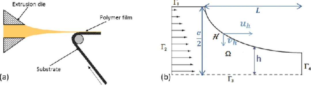
The considered coating process is used in several industrial processes such as coating and laminating. Polymer is driven in a flat die at high temperature and the extrudate is stretched at high draw ratio (above 200) on a very short distance (around 1 mm). The resulting thin polymer film is set down on a solid substrate to form a two-layer film (see Figure 1-a). A wavelike instability is observed through periodical variations in the thickness of the polymer film (draw resonance instability). It depends on processing conditions and it is obtained at draw ratios above a critical value. Numerical simulation of this process provides a better understanding of this instability.
FIGURE 1. (a) Schematic of the coating process, (b) Half flow domain of fluid
In the case of cast film process, Barq et al. identified the occurrence of draw resonance instability by measuring thickness and width fluctuations of the film as a function of time [1]. In the case of fiber spinning, when the stretching distance is increased, the critical Draw ratio Dr* increases, which is explained by non-isothermal effects [2,3,4]. Silagy et al. investigated the stability of the cast of film process using different constitutive equations. A membrane model has been considered and both linear stability analysis and direct numerical simulation have been employed [5]. In that case, increasing the drawing distance stabilizes the process. However, in our experimental studies, it was noticed that reducing the stretching distance to the order of the die gap considerably improves the stability of the process. This finding was proved by Souli et al. in the case of fiber spinning by using a 2D model and a tracking strategy combined with the linear stability method [6].
In this paper, we study the flow of polymer melt between the extrusion die and the substrate during stretching (Figure 1). Since the stretching distance is of the order of die gap, thin shell assumption is no longer valid. A 2D model in the thickness of the polymer film is considered instead. Numerical two-dimensional and time-dependent models are developed to investigate the onset of draw resonance instability. A boundary-value problem with a free
surface for the Stokes equations is considered and stability of the free surface is assessed using two different numerical approaches : the first one consists in a tracking strategy combined with a linear stability tool involving computation of leading eigenvalues, while the second approach is a direct simulation method involving a Level Set capturing strategy coupled with transient stability analysis. The novelty of this work is the ability to use a stabilized finite element anisotropic meshing coupled with a Level Set method to assess interface stability in coating processes.
GOVERNING EQUATIONS
Stokes Problem
Inertia and gravitational forces are neglected, isothermal problem with a Newtonian behavior is considered. Moreover, this model does not account for surface tension at fluid interfaces because it is considered negligible comparing to drawing forces [7]. Therefore, the momentum equations are given by :
⃗⃗ (1)
where is the Cauchy stress tensor defined by :
̇( ⃗⃗ ) (2)
and
⃗⃗
*
+
is the velocity vector, ̇( ⃗⃗ ) is the rate of deformation tensor, is the dynamic viscosity of the fluid and p is the pressure inside the fluid.In addition, the fluid is assumed to be incompressible, so we have :
⃗⃗ ⃗⃗ (3)
The Boundary Conditions
The applicable boundary conditions are given by :
At the wall 1 : ⃗⃗ ⃗ (no-slip condition)
On 2, a Poiseuille flow velocity field is imposed
On 3, we have symmetry conditions
On 4, take-up velocity is imposed
On the free surface H, two different boundary conditions are considered: the first condition assumes a zero stress at the free surface ⃗ , while the second condition is a non-miscibility condition and it is given by ⃗⃗ ⃗ , where ⃗ ,1) is a normal vector to the free surface.
In general, the draw ratio is a dimensionless number that can be defined as follows: ∫
∫
(4)
PROBLEM SOLVING
The interface-tracking and the interface-capturing techniques are both used in the computation of flow problems with moving boundaries and interfaces [8]. The Stokes problem is discretized and solved using a classical stable mixed-formulation (MINI element). All the implementation details are given in the following section.
Tracking Strategy
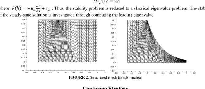
An interface-tracking technique requires moving meshes that “track” the interfaces and are updated as the flow evolves [8]. Therefore, we consider only the half flow domain of fluid Figure 1-b). For the resolution, we use a structured mesh and apply a transformation to refine it around the die exit singularity (see Figure 2).
The velocity and the pressure fields are then computed on this structured mesh which is restricted to the polymer flow. Interface with air is determined by successive iterations of Newton-Raphson’s method (by adjusting the position of the nodes on the interface) to satisfy the kinematic interface equation given by :
where ( ) is the velocity vector at interface and h is the interface position. This strategy is relatively precise but it is unable to describe transient evolution of the interface. The linear stability method is then used to predict onset of draw resonance. Since free surface is the only time-dependent variable, the steady state interface solution undergoes a perturbation of the form :
̅ ̂ (6)
where ̅ is the steady-state interface solution and ̂ is a perturbation of the interface. Therefore, the kinematic
interface equation is linearized near the steady state interface solution, which gives the following linearized equation:
( ̅) ̂ ̂ (7)
where . Thus, the stability problem is reduced to a classical eigenvalue problem. The stability of the steady-state solution is investigated through computing the leading eigenvalue.
FIGURE 2. Structured mesh transformation
Capturing Strategy
The interface between the air and liquid is now captured by solving a convected Level-Set function as introduced in [9, 10]. The basic idea of this method is to use both the physical time and the convective time derivative in the classical Hamilton-Jacobi reinitialisation equation. Consequently, a modified level-set function is given first as follows: { | | (8)
where stands for the standard distance function, and E is the truncation thickness. The level-set evolution equation is then given by:
(| | √ ( ) ) (9)
where is a coupling constant depending on time discretisation and spatial discretisation, typically and is the convection velocity. Finally, the authors in [10] show that by setting
| | and √ , a rearranged form of (9) leads to the following simple convection equation:
(| | √ ( ) ) (10)
The finite element formulation for the level set method is based on the use of the classical SUPG (Streamline upwind Petrov-Galerkin) method. It controls the spurious oscillations in the advection dominated regime. In brief, the finite element formulation of equation (10) can be written as follows: find , such that,
∫ ( ) ∫
∑ ∫ ( )
(11) where and are standard test and weight finite element spaces.
The classical Galerkin terms are represented by the first two integrals whereas the element-wise summation, tuned by the stabilization parameter , represents the SUPG term needed to control the convection in the streamline
direction. Once the level-set function is defined all over the domain, it can be used to easily separate both polymer and surrounding air phases. At the interface, the sharp discontinuity of the viscosity is smoothed over a transition thickness using the following expressions:
( ) {
( ( )) | |
(12)
where H is a smoothed Heaviside function. Here is a small parameter such that , known as the interface thickness, and is the mesh size in the normal direction to the interface. Combined with anisotropic mesh adaptation, it leads to an accurate and precise multiphase flow framework (see [10] for details).
NUMERICAL RESULTS AND DISCUSSION
In this section, two case studies are presented and analyzed. In the first case, we check the steady-state solutions obtained by both tracking and capturing techniques for a draw ratio of 18. In the second case study, we investigate the stability of the steady-state solution using a draw ratio of 10. The leading eigenvalue in each case are then computed and compared. In both cases, a shape factor is considered (Figure 1-b).
Steady-State Solution
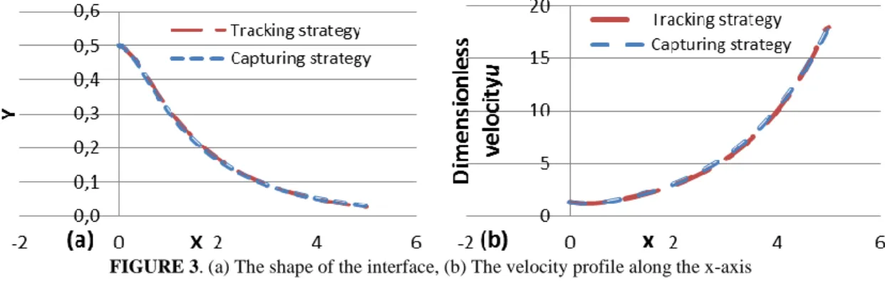
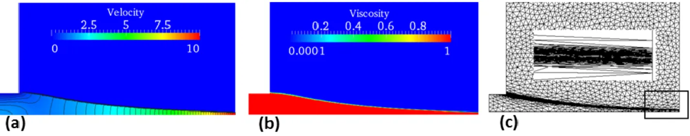
Figure 3-a shows a comparison for the shape of the interface at the steady-state obtained by both strategies. We can clearly see that both methods are able to converge to the same solution. This is also confirmed by comparing the velocity profiles along the x-axis (figure 3-b). Using the capturing strategy, we solve a multiphase Stokes problem that accounts for both polymer and air. Figures 4-a and 4-b highlight the velocity and the viscosity distribution all over the domain. As expected, the use of anisotropic mesh adaptation allows capturing precisely the polymer-air interface and thus leading to very accurate solution.
FIGURE 3. (a) The shape of the interface, (b) The velocity profile along the x-axis
Stability of the free surface
In this section, the stability of steady state solution is investigated for a draw ratio of 10 and a shape factor . In the case of tracking strategy, stability analysis is conducted by computing the leading eigenvalue as explained above. The free surface is stable only if the real part of the leading eigenvalue is negative. At those conditions, a leading eigenvalue is obtained meaning that the process is stable. In the case of capturing strategy, the transient stability analysis is performed by introducing a small perturbation to the steady-state solution. The transient response due to this perturbation is followed by the direct simulation, taking into account both domains, the polymer fluid and the surrounding air. Therefore, we can capture the evolution of the final thickness of the film as depicted in figure 5-a. The real part of the leading eigenvalue is estimated from the exponential envelope of the transient response while its imaginary part is estimated from oscillation’s time period. A leading eigenvalue of is obtained for the same conditions. This finding shows that both strategies were able to give the same stability results using two different stability analysis techniques. Figure 5-b shows that, at a
draw ratio of 18, the leading eigenvalue decreases when the shape factor decreases. Thus, reducing the stretching distance improves the stability of the coating process.
FIGURE 4. (a) Velocity profile, (b) The viscosity distribution, (c) The obtained mesh
FIGURE 5. (a) Transient stability analysis, (b) Leading eigenvalue evolution as a function of
CONCLUSIONS
The coating process was accurately simulated using tracking and capturing techniques and its stability was investigated. It was demonstrated that reducing the stretching distance improves the process stability. This corresponds to some experimental evidence. Future work will concern the development of models accounting for a pressure differential between the two sides of the polymer film and more realistic constitutive equations.
ACKNOWLEDGMENTS
The authors gratefully acknowledge Bostik S.A. company for experimental and financial support.
REFERENCES
1. P. Barq, J.M. Haudin, J.F. Agassant, P. Bourgin, “Stationary and dynamic analysis of film casting process, Intern. Polym. Proc. 9, 350-358 (1994).
2. L.L. Blyler and C. Gieniewski, “Melt spinning and draw resonance of a poly(-methylstyrene / silicone) block copolymer” in Polym. Eng. Sci., 140-148 (1980).
3. R.K. Gupta, P.D. Drechsel, “Draw resonance in the non-isothermal spinning of polypropylene”, 2nd World Congress of Chemical Engineering, Montréal, 1981.
4. Y. Demay, “Instabilité d’étirage et bifurcation de Hopf”, Thèse de Doctorat d’Etat, Université de Nice, 1983.
5. D. Silagy, Y. Demay, J.F. Agassant, “Stationnary and stability analysis of the film casting process”, J. Non-Newt. Fluid Mech. 79, 563-583 (1998)
6. M. Souli, Y. Demay, A. Habbal, “Finite element study of the draw resonance instability”, Eur. J. Mech., B/Fluids 12, 1-13 (1993).
7. A. Fortin, P. Carrier, Y. Demay, “Numerical simulation of coextrusion and film casting”. Int. J. Numer. Meth. Fluids 20, 31-57 (1995).
8. T.E. Tezduyar, “Interface-tracking and interface-capturing techniques for finite element computation of moving boundaries and interfaces”, Comput. Methods Appl. Mech. Engrg. 195, 2983–3000 (2006).
9. L. Ville, L. Silva, T. Coupez, Convected level set method for the numerical simulation of fluid buckling, Int. J. Numer. Meth. Fluids 66, 324-344 (2011).
10. E. Hachem, G. Francois and T. Coupez, Stabilised Finite Element for high Reynolds number, LES and free surface flow problems. In: Navier-Stokes Equations: Properties, Description and Applications, (Nova Science Pub Inc. )pp. 150-169, 2011