HAL Id: hal-00516832
https://hal.archives-ouvertes.fr/hal-00516832
Submitted on 11 Sep 2010
HAL is a multi-disciplinary open access
archive for the deposit and dissemination of sci-entific research documents, whether they are pub-lished or not. The documents may come from teaching and research institutions in France or abroad, or from public or private research centers.
L’archive ouverte pluridisciplinaire HAL, est destinée au dépôt et à la diffusion de documents scientifiques de niveau recherche, publiés ou non, émanant des établissements d’enseignement et de recherche français ou étrangers, des laboratoires publics ou privés.
Matching frictions, unemployment dynamics and the
cost of business cycles
Jean-Olivier Hairault, François Langot, Sophie Osotimehin
To cite this version:
Jean-Olivier Hairault, François Langot, Sophie Osotimehin. Matching frictions, unemployment dy-namics and the cost of business cycles. Review of Economic Dydy-namics, Elsevier, 2010, 13 (4), pp.759-779. �10.1016/j.red.2010.05.001�. �hal-00516832�
Matching frictions, unemployment dynamics and the cost of
business cycles
Jean-Olivier Hairault
Paris School of Economics (PSE) & Paris 1 University & IZA joh@univ-paris1.fr
Franc¸ois Langot
GAINS-TEPP (Le Mans University) & ERMES (Paris 2 University) & IZA flangot@univ-lemans.fr
Sophie Osotimehin ∗
CREST-INSEE & Paris School of Economics (PSE) & Paris 1 University sophie.osotimehin@ensae.fr
May 11, 2010
Abstract
We investigate the welfare cost of business cycles implied by matching frictions. First, using the reduced-form of the matching model, we show that job finding rate fluctuations generate intrinsically a non-linear effect on unemployment: positive shocks reduce unem-ployment less than negative shocks increase it. For the observed process of the job finding rate in the US economy, this intrinsic asymmetry increases average unemployment, which leads to substantial business cycles costs. Moreover, the structural matching model embeds other non-linearities, which alter the average job finding rate and consequently the welfare cost of business cycles. Our theory suggests to subsidizing employment in order to dampen the impact of the job finding rate fluctuations on welfare.
Keywords: Business cycle costs, unemployment dynamics, matching
JEL Codes: E32, J64
∗We thank Paul Beaudry, Guy Laroque, Etienne Lehmann, Franck Portier and Christian Zimmermann and all participants at the following seminars and conferences for helpful comments: Crest (2008), PSE (2009), Boston College (2009), British Columbia (2009), Boston University (2009), UQAM (2009), Malaga (2009), ZEW (2009) and SED (2009). This paper is a revised version of the IZA Working Paper 3840. Any errors and omissions are ours.
1
Introduction
In a very famous and controversial article, Lucas (1987) argues that the costs of business cycles are negligible: using empirically plausible values for risk aversion, he shows that individuals would only sacrifice a mere 0.008% of their consumption to get rid of all aggregate variability in consumption. This result is completely at odds with the neoclassical synthesis and the Keynesian legacies, but also, to a lesser extent, with a recent literature that documents far larger costs of business cycles (Beaudry and Pages (1999), Krebs (2007), Storesletten et al. (2001), Barlevy (2004), De Santis (2007) and Krusell et al. (2009)).
Our objective in this paper is to show that the matching unemployment theory may also lead to sizable welfare costs of business cycles. Due to strong non-linearities, average employment and therefore average consumption are lowered by the mere process of alternate expansions and contractions: the losses during recessions outweigh the gains during economic booms. The welfare cost of unemployment fluctuations stemming from these non-linearities has been ignored despite the high interest in the recent literature with matching frictions for the cyclical volatility of unemployment (Shimer (2005) and Hall (2005b)) and for the design of the optimal monetary policy (Blanchard and Gali (2008), Faia (2009) and Sala et al. (2008)). By filling this gap, our paper adds a new dimension to the analysis of the matching model with aggregate uncertainty. Following Cole and Rogerson (1999), our analysis is firstly based on the reduced form of the matching model where the job finding and separation rates are considered as exogenous stochas-tic processes. Focusing on the stock-flow unemployment dynamics allows us to emphasize that the core mechanism underlying our result does not depend on the structural matching consid-ered. Moreover, it clearly unveils the very different implications of fluctuations in the job finding rate and the separation rate for the costs of business cycle. During booms, the increase in the job finding rate is partly offset by the decrease in unemployment. In recessions, the decrease in the job finding rate is amplified by the increase in unemployment. Because of this asymmetry, aver-age unemployment is increased by fluctuations in the job finding rate. Conversely, fluctuations in the job separation rate lower the average unemployment rate1. However, we show that the impact of the volatility in the separation rate on the business cycle cost is necessarily one order of magnitude lower than that of the volatility in the job finding rate for the same coefficient of variation. Although Fujita and Ramey (2008) have recently shown that the relative contribu-tion of the separacontribu-tion rate to the unemployment volatility is higher than initially established by Shimer (2004), the impact of job separation fluctuations on the average unemployment rate, and then on the business cycle costs, is intrinsically limited. For the observed process of the job finding rate in the US economy, we show that the asymmetry quantitatively matters and generates sizable employment loss.
1During booms, the decrease in the job separation rate is amplified by the increase in employment. In recessions,
However, this reduced form approach suffers from several shortcomings. First, beyond the employment loss, one needs a better founded criterion in order to evaluate the business cycle cost. Secondly, the reduced form analysis supposes that business cycles do not have any effect on the average job finding rate: the counterfactual stabilized job finding rate is assumed to be equal to the average job finding rate. Finally, in the reduced form approach, stabilization policy cannot be explicitly addressed, as there is no operative way of getting rid of the cycles. A structural matching model is then necessary to take into account how the shocks hitting the fundamentals of the economy affect the job finding rate2. However, since Shimer (2005),
it is well known that the standard matching model fails to generate realistic fluctuations in the job finding rate. The studies aiming at elucidating the Shimer puzzle emphasize different mechanisms and none seems to close the debate3. Costain and Reiter (2008) have recently
emphasized that no calibration permits the standard matching model to be consistent both with business cycle facts and with the effects of labor market policies. They show that sticky wages can improve the matching model’s performance by making the firm’s flow of surplus more pro-cyclical, but Pissarides (2007) emphasizes that the observed proportionality between wages in new matches and labor productivity is then not replicated. Despite these remaining quantitative shortcomings, we believe it is interesting to investigate the welfare implication of unemployment volatility in the matching model as it adds a normative dimension to solving the Shimer puzzle.
We choose to study the business cycle cost implied by a matching model with wage rigidity as suggested initially by Hall (2005b) in a first response to the puzzle. This framework fits perfectly well with our objectives: it allows us to replicate all the volatility in the job finding rate4, but also to reveal, in a very transparent way, the basic non-linearity embedded in the
matching model. We show that the matching model naturally predicts that the job finding rate is a concave function of the vacancy-unemployment ratio. This could imply that fluctuations decrease the average job finding rate. But as the vacancy-unemployment ratio is a convex function of productivity, the impact of productivity fluctuations on the average job finding rate
2The Lucas’ approach can be considered as sharper than ours because it is model-free. But it cannot address
the stabilization issue.
3Hall (2005b) and Shimer (2005) initially proposed a rigid wage approach, which has been reconsidered more
recently by Hall and Milgrom (2008). This hypothesis increases the sensitivity of the model to productivity shocks, but at the expense of the observed flexibility in wages (Pissarides (2007)). Hagedorn and Manovskii (2008) show that a higher parametrization for the utility of being unemployed and a lower bargaining power for workers enable the standard matching model to yield realistic fluctuations in the unemployment rate. Whereas Hornstein et al. (2007) introduce investment-specific technological shocks, Kennan (2006) emphasizes the role of procyclical informational rents: the gain that firms obtain by being more informed than workers increases in booms. The inclusion of turnover costs (Pissarides (2007), Mortensen and Nagypal (2003) and Silva and Toledo (2008)) and match-specific technological change (Costain and Reiter (2008)) have also been investigated.
4Note that we choose to replicate all the volatility in the job finding rate only with productivity shocks, even
if it is now well-established that the volatility generated by these shocks only is lower (Pissarides (2007) and Mortensen and Nagypal (2003)).
is a priori ambiguous. These non-linearities come from the decreasing marginal returns in the matching function. The matching elasticity to vacancy plays a crucial role in the size of the business cycle costs: the lower the elasticity, the lower the average job finding rate and the higher the business cycle costs. The internal mechanisms of the matching model then lead to quite strong additional business cycle costs when the vacancy elasticity of the matching function is sufficiently low.
In order to show the robustness of our results, we propose two very different exercises. We firstly consider the flexible wage approach proposed by Hagedorn and Manovskii (2008). The employment loss is of the same magnitude as in the rigid-wage model, since the unemployment dynamics and the decreasing marginal returns are key features of any matching model. Secondly, using the panel data constructed by Bassanini and Duval (2006) over the period 1982-2003 for 20 OECD countries, we provide evidence that countries in which productivity is more volatile have also a higher level of unemployment.
All in all, the matching model with aggregate productivity shocks may challenge Lucas’s con-troversial view on welfare costs of business cycles. For the US economy, these costs reach 0.55% of permanent consumption for a calibration we consider as empirically relevant. However, this result is obtained under several conditions which deserve to be emphasized. Firstly, it implies to consider an expanded definition of unemployment which induces a higher volatility along the cycle, but also a higher level of structural unemployment. Secondly, the employment loss must be costly enough in terms of consumption: it implies that the surplus from market production is high enough. Typically, the high level of home production implied by the calibration proposed by Hagedorn and Manovskii (2008) for solving the Shimer puzzle leads to less significant welfare costs than the rigid-wage approach.
Finally, we explicitly address the policy issue. Besides stabilizing the job finding rate, our theory suggests dampening the impact of the job finding rate fluctuations on welfare, by subsidizing employment in order to increase the average job finding rate. Note that such subsidies in our model, characterized by a suboptimal level of employment, permit to reach both the stabilization and the resource allocation objectives.
The literature following Lucas (1987) has mostly focused on the consequences of business cycles on the volatility of individual consumption. More precisely, because business cycles amplify individual income risks, they could generate higher welfare losses than Lucas’s predictions when financial markets are incomplete. However, in as far as individual income fluctuations are transitory, the costs of the business cycle are still low, even negligible (Krusell and Smith (1999)), mainly because consumption can be smoothed through capital accumulation. On the other hand, when individual income variations are more persistent, the cost of business cycles becomes more substantial, at least 1% percent of the permanent consumption (Beaudry and Pages (1999), Krebs (2007), Storesletten et al. (2001), De Santis (2007), Krusell et al. (2009)). Reis (2009)
shows that the persistence also plays a key role when only aggregate shocks are considered. In the literature, very few papers focus on the consequences of business cycles for average consumption. This idea has been sketched out by De Long and Summers (1988); they argue that rather than steadying economic activity at its average level, stabilization would prevent output from deviating from its potential level. Ramey and Ramey (1993) explore this mechanism in a model where firms have to pre-commit to a specific technology before starting production. Stabilization may also increase welfare through its effect on capital accumulation (Matheron and Maury (2000), Epaulard and Pommeret (2003) and Barlevy (2004)). Finally, a very recent paper by Jung and Kuester (2008) emphasizes the non-linear relation between unemployment and the job finding rate. They, however, propose a quite complex matching model with capital accumulation, liquidity constraints and human capital, which prevents them from clearly evaluating the basic non-linearities embedded in the matching approach. Moreover, all these additional features bring very small business cycle costs. This shows a clear difference from our paper: we aim at unveiling in the basic matching model the mechanisms which lead to business cycle costs, namely the stock-flow unemployment dynamics and the congestion effects due to decreasing marginal returns in the matching function. Although the implied business cycle costs are weaker than in recent studies (Krebs (2007), Reis (2009) and Barlevy (2004) for instance), the effect of aggregate fluctuations on the employment level adds to the list of factors missing from Lucas’s argument, and would indicate more substantial welfare costs from business cycles.
The paper is organized as follows. Section 2 uses a reduced form of the matching model to investigate the consequences of the non-linearity in the unemployment dynamics. Section 3 takes into account the non-linearity in the job finding rate dynamics embedded into the matching model. The fourth section is devoted to robustness tests. The last section concludes.
2
Asymmetry in the unemployment dynamics: a reduced form
approach
Labor market frictions naturally generate asymmetries in the unemployment dynamics. Because of these asymmetries, aggregate fluctuations may have an impact on average unemployment. In this section, following Cole and Rogerson (1999), our theoretical framework is based on the reduced form of the matching model. The use of a reduced form model has the advantage of emphasizing that these asymmetries are present in any labor market matching model. We first present our theoretical framework, and then analyze the unemployment dynamics. Finally, a preliminary quantitative evaluation of the business cycle costs is proposed.
2.1 Framework
We consider unemployment dynamics as the result of exogenous job separation and job finding fluctuations. By shutting down any non linearities5 that may affect the job finding and
sepa-ration rates, the reduced form model allows us to focus on the non linearity embedded in the unemployment dynamics.
Unemployment. The unemployment dynamics arise from the entries to and exits from em-ployment. The former are determined by the job finding rate p, the latter by the separation rate
s.
ut+1= st(1 − ut) + (1 − pt)ut (1)
Shocks. The economy is hit only by aggregate shocks which generate some fluctuations in the job finding rate pt and in the separation rate st. The job finding rate and separation rate
are exogenous with respect to u. This key assumption derives from the matching theory. The aggregate shocks affect linearly both the job finding rate and the separation rate which are assumed to follow an AR(1) process6:
pt = (1 − ρp)¯p + ρppt−1+ εpt (2)
st = (1 − ρs)¯s + ρsst−1+ εst (3)
The shocks εpand εshave a zero-mean and a standard deviation equal to σ
εpand σεs respectively.
¯
p and ¯s denote the average job finding rate and the average separation rate respectively.
Business cycle costs. Aggregate shocks may cause average unemployment to differ from the level it would have reached in an economy without any shocks. Following the convention in the literature, we refer to the latter as the stabilized economy. How the stabilized economy is reached is not explicitly presented. In particular, nothing is said in this section on the design and the efficiency of stabilization policies.
The cost of fluctuations is the cost of being in an economy hit by aggregate shocks, rather than being in an economy without aggregate shocks. In the former economy, the job finding rate and the separation rate fluctuate around their means, whereas in the latter they are set forever at their average value ¯p and ¯s. The stabilized unemployment (or the structural unemployment) is
equal to:
¯
u = s¯
¯
s + ¯p
5We will show in the structural approach (Section 3) that the average job finding rate can be increased or
decreased by aggregate fluctuations. The job finding rate is a concave function of the vacancy-unemployment ratio, but, as the vacancy-unemployment ratio is a convex function of productivity, the effect of productivity fluctuations on the average job finding rate is a priori ambiguous. The reduced form case, in which fluctuations do not affect the average job finding rate, can then be considered as an instructive benchmark.
6We assume symmetrical shocks in order to identify the endogenous asymmetries generated by equation (1).
The percentage of aggregate employment lost in the business cycle is then given by:
λu = 1 − ¯u
1 − E(u)− 1 =
E(u) − ¯u
1 − E(u)
with E(u) the unconditional expectation of unemployment. Traditionally, since Lucas (1987), the business cycle cost is defined as the percentage of the consumption flow that agents would accept sacrificing in order to get rid of aggregate fluctuations. To what extent employment losses are transformed into welfare costs depends on the links between employment, income and consumption. This issue requires a more structural approach and we will show in Section 3 that the employment loss can be considered as a good approximation of the welfare costs in a matching economy. But it is already straightforward that the employment loss λu is of the same order of magnitude as the welfare cost in an economy populated by risk-neutral agents without savings.
2.2 The analysis of the non-linearities in the unemployment dynamics
By considering equation (1), it is fairly intuitive that shocks on the job finding rate and on the separation rate have non linear effects on unemployment. The impact of these shocks depends on the level of unemployment. During booms, the decline in unemployment offsets the increase in the job finding rate. The small search pool in booms implies that a higher job finding rate increases job creations less than it otherwise would. On the contrary, as unemployment is higher during a recession, the job finding rate shocks have a greater impact in recession; the decline in the job finding rate is magnified by the increase in unemployment. As a result, fluctuations in the job finding rate tend to increase average unemployment.
Conversely, as the impact of the job separation rate shocks depends on the level of employ-ment, the fluctuations in the separation rate lead unemployment to decrease more in booms than to increase in recession: fluctuations in the job separation rate tend to reduce average unemployment.
In this section, we assess precisely these different effects. First, as it is traditionally done in the matching approach with aggregate shocks (see for instance Hall (2005)), a steady state analysis of equation (1) is conducted and so fluctuations in the conditional steady states are considered. This analysis delivers very easily the basics of the non-linearity embedded in the unemployment dynamics. This simple framework highlights the importance of the volatility of the job finding and separation rates for the size of business cycle costs, but also the less expected role played by the structural unemployment rate. Secondly, taking into account the inertia embedded in equation (1), we derive the full non-linear properties of the unemployment dynamics and show that the persistence of the aggregate shocks also matters.
2.2.1 Steady state analysis
Let us assume for now that the speed of convergence of unemployment is infinite: fluctuations cause unemployment to jump directly from one conditional steady state to another. A condi-tional steady state unemployment corresponds to the level eui toward which the unemployment
rate would converge if the separation and job finding rates forever keep the same value pi and si,
i.e. if the economy remains in the same state i. Let us define πi the unconditional probability
of being in state i. The value taken by p and s in each state i and the probability associated
πi define the Markov chains associated with p and s, consistently with equations (2) and (3). The average job finding rate ¯p is therefore equal to Piπipi and the average separation rate ¯s
toPiπisi. Jointly, they determine the structural unemployment rate ¯u. On the other hand, as
unemployment is assumed to jump directly from one conditional steady state to another, the average unemployment in this economy is then equal to the average of the conditional steady states:
˜
u =X
i
πiuei
The non-linearity embodied in equation (1) implies that average unemployment ˜u has no reason
to coincide with structural (stabilized) unemployment ¯u.
Job finding rate shocks
To understand the specific role of the non linearity in job findings, let us assume first that the separation rate is constant and equal to its mean ¯s. This non-linearity implies that eui is a convex
function of the state-dependent job finding rate pi: e
ui= s + p¯ s¯ i
(4) Because unemployment is a convex function of the job finding rate, the average unemployment is higher than the structural (stabilized) unemployment ¯u. For uniformly small deviations, using
a second order Taylor expansion of equation (4), this gap can be written as 7:
˜ u − ¯u ≈ ¯u (1 − ¯u)2 µ σp ¯ p ¶2 (5) A mean-preserving increase in the volatility widens the gap between the stabilized and fluctu-ating unemployment rates. The more volatile the economy, the greater the business cycle cost. Equation (5) indicates that the unemployment gap also depends on the structural unemploy-ment rate ¯u. This result is important as it generates strong interactions between structural and
cyclical unemployment. More particularly, a higher value of ¯u imply a more convex economy and
leads to higher business cycle costs8. Furthermore, this suggests that labor market institutions
7See Appendix A for the derivation. 8This holds as long as ¯u ≤ 1/3.
affect the costs of fluctuations as they have an impact on the average job finding and separation rates.
Job separation rate shocks
So far, the separation rate was assumed to be constant. However, it appears clearly from equation (1) that the asymmetry in the unemployment dynamics could also come from fluctuations in the separation rate. The resulting unemployment gap would then read:
e u − ¯u ≈ −¯u2(1 − ¯u)³ σs ¯ s ´2 (6) with σs the unconditional standard deviation of the separation rate. Contrary to the job finding
rate case, fluctuations in the separation rate tend to reduce average unemployment. Job sepa-rations decrease more in expansion than they increase in recessions. As shown by equation (6), the unemployment gap depends again on the average job finding and separation rates: a higher structural unemployment rate leads to more business cycle gains9. Further, the asymmetry
embodied in equation (1) translates into average unemployment only if the separation rate is volatile enough.
2.2.2 Considering unemployment inertia
All previous calculations have been made with the assumption that unemployment jumps directly to the conditional steady states. Under this assumption, average unemployment in the business cycle economy is equal to the average of the steady states. Because of unemployment inertia, the asymmetry embodied in the conditional steady state does not necessarily manifest in average unemployment. This asymmetry affects the average unemployment rate only if the aggregate shocks are persistent enough.
To see in a synthetic formula the role of the mean, the volatility and the persistence of aggre-gate shocks, let us solve equation (1). Again, we first compute average unemployment in the case where only the job finding rate is fluctuating. As shown in Appendix B, the additional unemployment created by business cycles can then be approximated by 10:
E[u] − ¯u ≈ (1 − ¯u)2 s ρ¯ p 1 − ρp(1 − ¯s − ¯p) µ σp ¯ p ¶2 (7) If pt was not serially correlated (ρp = 0), fluctuations in the job finding rate would not affect
average unemployment: E[u] = ¯u. When aggregate shocks are persistent, average unemployment
9This holds for ¯u ≤ 2/3.
10The approximation consists of neglecting moments of order above 2. This is line with our approach : as we
want to understand how symmetrical shocks can yield non symmetrical effects on unemployment, we disregard in particular the consequences of non-zero skewness
in the business cycle economy is no longer equal to stabilized unemployment. In line with our intuition, equation (7) also shows some interactions between the job finding rate volatility, its persistence and the structural unemployment rate. An increase in the variance of the shocks raises average unemployment all the more so when the average job finding rate is low and the persistence of the shocks is high.
Symmetrically, in the case where only the separation rate is fluctuating, the gain of fluctuations positively depends on the volatility and on the persistence of the separation rate:
E[u] − ¯u ≈ −¯u2 p ρ¯ s 1 − ρs(1 − ¯s − ¯p) ³ σs ¯ s ´2 (8) Again, the structural unemployment rate interacts with the volatility and the persistence of the shocks. However, as shown by equations (7) and (8), the employment gains are potentially smaller than the employment losses for the same coefficient of variation and the same level of autocorrelation, since the unemployment rate is one order of magnitude lower than the em-ployment rate. Although Fujita and Ramey (2008) have recently established that the relative contribution of the separation rate to the unemployment volatility is higher than initially shown by Shimer (2004), the impact of job separation fluctuations on the average unemployment rate, and then on the business cycle costs, remains intrinsically limited11. This is why we disregard job separation fluctuations in the sequel.
2.3 Quantifying the employment loss
To investigate whether the observed fluctuations in the job finding affect average unemployment and hence the costs of business cycles, it is necessary to estimate the AR(1) process12 described
by equation (2). As equation (7) gives only an approximation of average unemployment, we resort to simulations to obtain a more accurate estimate of the costs of business cycles. Con-sistently with the AR(1) estimation, we simulate job finding rate shocks in order to obtain artificial series. We then use them to simulate equation (1), which allows us to compute the average unemployment rate in the business cycle economy and the business cycle costs13.
11The variance decomposition proposed by Fujita and Ramey is based on the linearization of steady state
unemployment: σ2 u ≈ (1 − ¯u)2u¯2 ·³ σp ¯ p ´2 +¡σs ¯ s ¢2 − 2ρs,pσ¯ssσp¯p ¸
. If the separation rate and the job finding rate were characterized by the same coefficient of variation, the variance decomposition indicates that the separation rate would contribute to half of the volatility in the unemployment rate, whereas the impact of fluctuations in the separation rate on the average unemployment rate would be much weaker than that of the job finding rate. In Hairault et al. (2008), we checked that the business cycle gains implied by the observed volatility of the job separation rate is not significantly different from zero.
12It must be emphasized that considering a log-normal distribution for p would have led to very similar results.
See Appendix D for more details.
13Note that we also need mean separation rate for simulating equation (1). It is estimated at 0.031 in Hall’s
2.3.1 Data
The behavior of the job finding rate over the business cycle is still a debated subject. It espe-cially depends on the underlying conception of “unemployment”. Contrary to Shimer (2005), Hall (2005a) uses a measure of unemployment expanded to include “discouraged workers” and “marginally attached workers”. Although those workers are classified as being out of the labor force, their behavior is close to that of workers classified as unemployed. Blanchard and Diamond (1990) advocate that the hazard rate for workers who are not in the labor force but “want a job” is similar to that of the unemployed workers. Their transition rate to employment is significantly higher than that of the other workers out of the labor force. For Canada, the transition rate to employment is 12.4% for marginally attached workers vs 3.5% for other non-participants and 23% for unemployed workers (Jones and Riddell, 2006). Although our benchmark result is based on Hall’s data, we also provide the results obtained when Shimer’s approach is used14, in order
to emphasize the sensitivity of the employment loss to this choice.
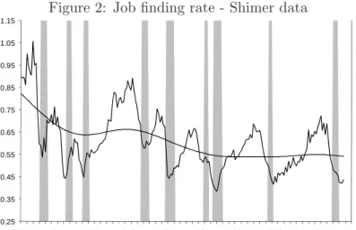
The Hall (2005a) and Shimer (2005) measures of the job finding rate both exhibit pro-cyclicality. The job finding rate plunges at each recession and recovers at each expansion (Figures 2 and 3, Appendix C). Both measures show a downward trend in the 1970s and in the early 1980s. As some of these movements could be due to factors unrelated to business cycles, we focus hereafter on series detrended by a low frequency filter.
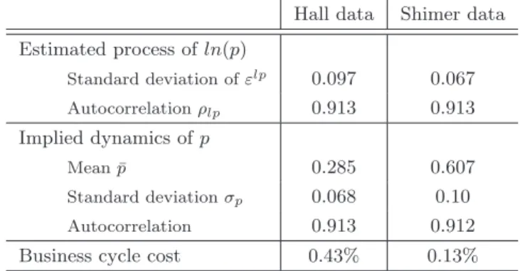
Table 1: Job finding rate statistics
Hall data Shimer data
Mean ¯p 0.285 0.607 Standard deviation σp 0.069 0.100 Coefficient of variation σp ¯ p 0.242 0.165 Autocorrelation 0.913 0.903
Note: Quarterly average of monthly data. Sample covers 1948q3-2004q3 for Hall (2005a) and 1951q1-2003q4 for Shimer (2005). Following Shimer (2005), both sets of data are detrended with a HP smoothing parameter of 105.
We then estimate the parameters characterizing the process of the job finding rate as described by equation (2). As expected, the “expanded job finding rate” has a lower mean than Shimer (2005)’s measure (Table 1). More importantly, including low-intensity job seekers also implies a higher coefficient of variation.
14Note that for Shimer’s series, we use the job finding and separation rates and not the job finding and separation
probabilities as the latter are not consistent with the stock flow equation for unemployment (equation (1)): Shimer (2005) takes into account the probability of finding another job within the month.
2.3.2 Simulation results
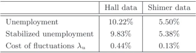
Table 2: Average unemployment and job finding rate fluctuations
Hall data Shimer data
Unemployment 10.22% 5.50%
Stabilized unemployment 9.83% 5.38% Cost of fluctuations λu 0.44% 0.13%
Table 2 presents the employment loss due to business cycles in the US economy for the two measures of the job finding rate. Non-linearities in the unemployment dynamics are enough to generate sizable costs of business cycles. In particular, these costs are between one and two orders of magnitude greater than the costs found by Lucas (1987)15. The method chosen to
measure the job finding rate has strong consequences on the costs of fluctuations. When some non-employed job seekers (Hall’s method) are taken into account, fluctuations in the job finding rate induce a 0.44% employment loss. Shimer’s measure leads to lower business cycle costs: if the job finding rate is computed using only transitions from unemployment, the cost of business cycles reduces to 0.13%. Such a result was expected, as Shimer’s job finding rate series display both a lower volatility and a higher mean (Table 1), two characteristics that we identified as cost-reducing.
3
Endogenizing the job finding rate: a structural approach
The previous section showed that the observed volatility and persistence in the job finding rate lead to sizable costs of business cycles. The structural matching model is a candidate for generating such costs. However, Shimer (2005) shows that the canonical matching model fails to generate realistic fluctuations in the job finding rate. The standard deviation of the job finding rate is much greater in the data than in the model (Shimer (2005)). An increase in labor productivity increases the expected profit from a filled job, and thus firms tend to open more vacancies. But there are internal forces in this framework which partially offset the initial increase in expected profits and then dampen the incentives for vacancy creations.
There already exist in the literature different approaches which solve the Shimer puzzle16. Do
we care about identifying the mechanism at the origin of the high fluctuations in the job finding
15At this stage, we agree that the two approaches are not directly comparable. We will see in the next section
that the employment loss is not so far from a cost expressed in terms of consumption.
16See for instance Hall (2005b), Hall and Milgrom (2008), Pissarides (2007), Hagedorn and Manovskii (2008),
Hornstein et al. (2007), Kennan (2006), Mortensen and Nagypal (2003), Silva and Toledo (2008) and Costain and Reiter (2008).
rate? From the analysis conducted in the first part, it could be tempting to say that it is enough to know that at least one theory is able to replicate the job finding rate dynamics. Actually, we do care. Indeed, the results obtained in the first part are derived from a model in which the job finding rate is exogenous, and in which fluctuations are neutral regarding the average job finding rate. To assess the costs of fluctuations, one must take into account the consequences of stabilization on the average job finding rate. If productivity shocks and the job finding rate are linearly related, the results found in the previous section should a priori be close to the endogenous job finding rate case. But if not, the average job finding rate can then be affected by business cycles. Why do we suspect the presence of a non-linear effect of business cycles on the job finding rate? The job finding rate is a non-linear function of the labor market tightness which also depends non-linearly on productivity changes. To show and quantify these different effects, a structural model is then required and the costs of business cycles could differ according to the model specification. This last statement is all the more true as the cost of business cycles will rely on a welfare criterion consistent with the structural model. In particular, more attention must be paid to the cyclical behavior of vacancies.
The choice of the theoretical model is then potentially crucial. We choose to study the business cycle cost implied by a canonical matching model with wage rigidity (Hall (2005b)). As in the previous section, we leave aside the fluctuations in the separation rate so as to keep the analysis as tractable as possible17. This approach allows us to focus on the implications of the basic
non-linearity introduced by the matching function. We then present different calibrations of the matching function elasticity in order to unveil these implications. Each replicates the job finding rate process (standard deviation and mean)18. The implied business cycle costs are
not necessarily identical and equal to that obtained in the reduced-form part. In a robustness analysis, considering a flexible wage framework (Hagedorn and Manovskii (2008)), we show that these mechanisms are intrinsic to the matching model, and then not specific to the rigid wage approach.
3.1 A canonical matching model
The model considered hereafter is a version of the matching model `a la Pissarides with aggregate uncertainty and exogenous separation.
17Moreover, it is well-known that job creation conditions are unaffected when job separations are endogenous
(Pissarides (2007)).
3.1.1 Matching technology
Output per unit of labor is denoted by ytand is assumed to follow a first-order Markov process
according to some distribution G(y, y0) = P r(y
t+1 ≤ y0|yt = y). To hire workers, firms must
open vacancies at unit cost κ. Jobs and workers meet pairwise at a Poisson rate M (u, v), where M (u, v) stands for the flows of matches and v the number of vacancies. This function is assumed to be strictly increasing and concave, exhibiting constant returns to scale, and satisfying
M (0, v) = M (u, 0) = 0. Under these assumptions, unemployed workers find a job with a
probability p(θ) = M (u, v)/u that depends on the ratio of vacancies to unemployment (θ = v/u). The probability of filling a vacancy is given by q(θ) = M (u, v)/v. Hereafter, we impose that the matching function is Cobb-Douglas: M (u, v) = ϕu1−αvα with 0 < α < 1.
The unemployment dynamics in the economy (equation (9)) are similar to equation (1), except that the job finding rate is now endogenous. Equations (10) and (11) define the job finding rate and the job filling rate respectively which depends19 on the current productivity state y:
u0 = s(1 − u) + (1 − p(θy))u (9)
p(θy) = ϕθyα (10)
q(θy) = ϕθyα−1 (11)
3.1.2 Workers
Workers are risk neutral. They have no access to financial markets. This simplifying assumption is not restrictive as our results do not rely on the impossibility of individuals smoothing their income. As agents are risk-neutral, the excessive volatility of consumption implied by this assumption is not captured in the welfare calculations. The focus is here on the impact of business cycles on average consumption, which is not affected by smoothing behaviors.
Workers can either be employed or unemployed. Employed workers receive wage w until their job is destroyed (at rate s); we do not take into account on-the-job search and voluntary quits. An unemployed worker gets an unemployment benefit20 z which is equally financed by workers
through lump-sum taxes. We choose to consider that the disutilities of working and of not working are both equal to the same value χ. It is then straightforward to derive the representative agent intertemporal preferences:
E0
∞
X
t=0
βt(ct− χ)
19Throughout the paper the notation x
y indicates that a variable x is a function of the aggregate productivity level y and Eyis the expected value conditional on the current state y.
20At this stage, the non market value does not include home production. See the robustness analysis for a
where E0 denotes the expectation operator conditional on information at time 0 and β the
discount factor.
3.1.3 Aggregate consumption and the welfare cost of business cycles
In our economy, aggregate consumption is equal to the aggregate production net of the vacancy costs.
ct= yt(1 − ut) − κ vt (12)
In this economy, the only sources of fluctuations are the labor productivity shocks. The welfare cost of fluctuations is therefore defined relatively to a counterfactual economy, in which labor productivity remains at its average value. The welfare cost of business cycles λ is defined as the percentage of the consumption flow that the agent would accept sacrificing in order to get rid of aggregate fluctuations: E0 ∞ X t=0 βt[(1 + λ)ct] = E0 ∞ X t=0 βt¯ct
where ¯ct is the level of consumption in the economy without aggregate shocks. It needs to be derived from a counterfactual experiment based on an artificial economy without any shocks. The computation of welfare costs takes explicit account of the transition path to the stabilized economy. However, in order to highlight the welfare cost of business cycles in the matching economy, let us consider the following expression, which leaves aside the transition path21:
λ ≈ ¯c − E(c)
E(c) =
[(1 − ¯u)¯y − κ¯v] − E[(1 − u)y − κv]
E(c) (13)
Business cycles are costly when they make the production net of the vacancy cost lower than its stabilized level. In order to make a link with the reduced form analysis, the welfare cost of business cycles can be written as follows:
λ ≈ (E(u) − ¯u) − cov(y, 1 − u) + κ(E(v) − ¯v)
E(c) (14)
The first part of the welfare cost of business cycles is the employment loss (E(u)−¯u) present in the
reduced-form analysis. Let us emphasize that the size of the employment loss is not necessarily of the same magnitude in the structural model, as the job finding rate is now endogenous. The lower the average job finding rate, the higher the employment loss and the higher the welfare cost. The second part cov(y, 1 −u) comes from the interaction between productivity and employment. Just as making the job finding rate negatively correlated with the stock of job searchers lowers mean employment, making productivity positively correlated with the stock of workers raises mean output. This explains why a positive covariance leads to decrease the business cycle costs. Finally, the third part shows that more vacancies in the fluctuating economy than in the stabilized one generate higher costs.
21The transition path does not significantly matter in our economy: it decreases the business cycle cost only
3.1.4 The value functions The worker’s utility
Define Uy and Wy to be the state contingent present value of an unemployed worker and an employed worker22:
Uy = z + β{(1 − p(θy))Ey[Uy0] + p(θy)Ey[Wy0]} (15) Wy = wy+ β{(1 − s)Ey[Wy0] + sEy[Uy0]} (16)
The firm’s surplus
The firm’s value of an unfilled vacancy Vy is given by:
Vy = −κ + β{q(θy)Ey[Jy0] + (1 − q(θy))Ey[Vy0]} (17)
with Jy the state contingent present value of a filled job and q(θy) the probability of filling a
vacancy conditionally on the productivity state y. When the job is filled, the firms operate with a constant return to scale technology with labor as only input. The firm’s value of a job is given by:
Jy = y − wy+ β{(1 − s)Ey[Jy0] + sEy[Vy0]} (18)
Free entry implies Vy = 0 for all y. Therefore, the job creation condition is:
κ = βq(θy)Ey[Jy0] (19)
3.1.5 Equilibrium
The labor market equilibrium depends on the way the wage is determined in the economy. Though our benchmark is the rigid wage model, we first present the traditional equilibrium with a Nash-bargained flexible wage. It allows us to compare the non-linearities embedded in these two equilibria.
Equilibrium with flexible wages.
When a worker and an employer meet, the expected surplus from trade is shared according to the Nash bargaining solution. The joint surplus Sy is defined by Sy = Wy+ Jy− Uy. The worker gets a fraction γ of the surplus, with γ her bargaining power. The equilibrium with flexible
22For the sake of simplicity, we omit from these equations the disutility of working and not working, the
lump-sum tax financing the unemployment benefits and the dividend paid by firms to workers, as these variables are assumed to be identical across individuals.
wages is defined by the job creation condition and the wage rule (equations (20) and (21)), plus equations (9) to (11): κ q(θy) = βEy · y0− w(θy0) + (1 − s) κ q(θy0) ¸ (20) w(θy) = γ(y + κθy) + (1 − γ)z (21)
As Shimer (2005) points out, the adjustment of wages is responsible for the insensitivity of the la-bor market tightness to the productivity shocks. It also makes the interplay of the non-linearities in the model more complex relative to the rigid wage equilibrium, due to the retroaction of wages in the job creation condition (equation (20)).
Equilibrium with rigid wages
Incorporating wage rigidity in the matching model is a natural way to generate enough volatil-ity. Moreover, this allows us to focus on the basic non-linearities introduced by the matching function, present in any matching model.
Following Hall (2005b), we consider a constant wage wy = w, ∀y. This constant wage is an
equilibrium solution if z ≤ w ≤ min πy, where πy denotes the annuity value of the expected
profit23. The wage is set at the Nash bargaining solution relative to the average state of
pro-ductivity ¯y. This wage is an equilibrium wage provided it lies in the bargaining set defined by
the participation constraints of the firms and the workers.
The rigid wage equilibrium is then defined by substituting equations (20) and (21) by equations (22) and (23), again in addition to the conditions (9) to (11):
κ q(θy) = βEy · y0− ¯w + (1 − s) κ q(θy0) ¸ (22) ¯ w = γ(¯y + κθy¯) + (1 − γ)z (23)
3.2 Non-linearities, welfare cost and employment loss: the rigid wage case
When wages are rigid, the employment loss can be considered as a good approximation of the welfare cost. Indeed, as the production net of vacancy costs is approximately equal to labor earnings (for a discount factor β sufficiently close to 1)24, it is straightforward to show that:
λ ≈ w(1 − ¯¯ u) − E( ¯w(1 − u))
E( ¯w(1 − u)) =
E(u) − ¯u
1 − E(u) (β → 1) (24)
23This annuity value is simply computed using the value an employer attaches to a new hired worker who never
receives any wage:
e
Jy= y + β(1 − s)Ey[ eJy0] The annuity value is then given by πy= [1 − β(1 − s)] eJy.
Comparing with equation (14), the cost-decreasing effect of the covariance between productivity and employment and the cost-increasing effect of higher vacancies compensate each other for a discount factor β sufficiently close to 1. More generally, the wage rigidity in the business cycles makes the welfare cost very close to the employment loss.
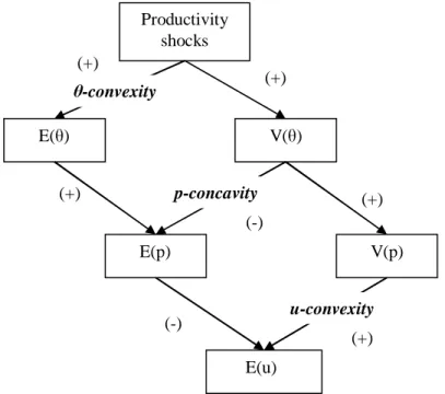
The total impact of productivity fluctuations on the average unemployment rate is then key to understand the business cycle costs. Figure 1 presents the mapping between labor productivity and unemployment. There is a first source of convexity arising from the unemployment dynamics (u-convexity effect), equation (9). It has been intensively investigated in the previous section. Let us concentrate here on the additional non-linearities that appear once p is endogenous. They determine altogether the average job finding rate and their global impact is not determined a priori.
Figure 1: Non-linearities in the structural matching model
Productivity shocks E(θ) E(p) V(p) E(u) V(θ) (+) (+) (+) (-) (+) (-) (+) p-concavity θ-convexity u-convexity
As the return of an additional vacancy on the job finding rate is decreasing (equation (10)), the average job finding rate in the stabilized economy is potentially higher than in a economy with business cycles (p-concavity effect). The lower the elasticity α of the matching function to va-cancies, the higher the p-concavity effect. Let us emphasize that this effect tends unambiguously to create higher welfare costs as the job finding rate is lowered by the volatility of the labor market tightness, and not by its level25. Average unemployment increases without any gains in
25In this latter case, a lower labor market tightness could be welfare-improving, if the deterministic equilibrium
terms of vacancy reductions.
On the other hand, equation (22), combined with the job filling rate condition (equation (11)), implies that the average labor market tightness is increased by productivity fluctuations. As the matching function exhibits decreasing marginal returns to vacancies, the average duration of a vacancy and hence the cost of opening a vacancy are concave in the labor market tightness. Therefore, the free entry condition is satisfied for greater variations in job creation in booms than in recessions: the labor market tightness is a convex function of productivity (θ-convexity effect). This effect tends to increase the average job finding rate in the fluctuating economy . From equation (11), it can be seen that this convexity is amplified by a high elasticity α of the matching function to vacancies. Ceteris paribus, it leads to lower business cycle costs only in the case where the deterministic equilibrium level of employment is below its optimal value. This is the case in our economy, whatever the parameters we consider, as we impose relatively high unemployment benefits.26
Overall, the way the productivity shocks affect the job finding rate on average depends on the degree of decreasing returns in the matching function captured by the elasticity α. To make this point explicit, let us approximate the unemployment rate using the comparative statics of the model without aggregate shocks27:
u ≈ u−u 2 s p 0(θ)θ0(y)(y−y)+u2 s µ u s £ p0(θ)θ0(y)¤2−1 2 £ p00(θ)(θ0(y))2+ p0(θ)θ00(y)¤ ¶ (y−y)2 (25)
The employment loss can then be expressed as follows28:
E(u) − ¯u ≈ ¯u (1 − ¯u)2 µ σp ¯ p ¶2 | {z } u-convexity −u¯ s 1 2 p00(¯θ)(θ0(¯y))2 | {z } p-concavity + p0(¯θ)θ00(¯y) | {z } θ-convexity σ2y | {z } E(p)−¯p (26)
The first part of the welfare cost of business cycle captures the impact of the job finding rate volatility on average unemployment (u-convexity). The second part comes from the impact of the productivity volatility on the average job finding rate. It combines both the p-concavity and the θ-convexity and thus depends on the elasticity α of the matching function to vacancies. This can be shown more formally as follows29:
p00(θ)(θ0(y))2+ p0(θ)θ00(y) = Γ(θ)(2α − 1) Γ(θ) > 0
The stabilization of labor productivity either decreases or increases the average job finding rate, depending on the value of the elasticity of the matching function α. The job finding rate is
26Note that this is a conservative choice with regard to the size of the business cycle costs.
27The comparative static of the model without aggregate shocks can be used to approximate the dynamic
stochastic model if the shocks are persistent enough. See Mortensen and Nagypal (2003) for more details.
28As p = ¯p + p0(θ)θ0(y)(y − ¯y) +1 2(p 00(¯θ)(θ0(¯y))2+ p0(¯θ)θ00(¯y))(y − ¯y)2. 29Γ(θ) = ϕα (1−α)2 ³ β κ(1−β(1−s)) ´2 θ3α−2.
a concave (convex) function of labor productivity if α is below (above) 1/2 and the stabilized job finding rate is then higher (lower) relatively to that of the volatile economy. In the case
α = 1/2, the θ-convexity and the p-concavity effects exactly compensate each other. In this
case, the productivity fluctuations will lead to the same increase in average unemployment as in the reduced form analysis.
These basic non-linearities are not specific to the rigid wage model. It is obvious that the flexible wage equilibrium shares the same fundamental non-linearities, as they stem from the intrinsic characteristics of the unemployment dynamics, of the job finding rate and of the job filling rate which are exactly the same in the two equilibria. However, in the flexible wage case, the θ-convexity effect is modified by the retroaction of the wage in the job creation condition (equations (20) and (21)). Hence, the non-linearity between y and θyalso depends on the assumption about
the wage bargaining process, and more generally on the particular assumptions considered, such as the existence or not of fixed hiring and separation costs. In this sense, the flexible wage equilibrium may introduce non-linearities which are not intrinsic to the matching process. The use of the rigid wage framework allows us to focus on the basic non-linearities which are common to a large class of matching models.
3.3 Quantifying the business cycles costs
We first calibrate the rigid wage economy. As equations (24) and (26) give only an approximation of the welfare cost of business cycles, we resort to simulations to obtain an accurate estimate.
3.3.1 Calibration
The model is calibrated to match US data. We calibrate the productivity process to match the US labor productivity standard deviation and persistence30. The monthly discount rate is
set to 0.42%. The job separation rate is set at Hall’s estimate for the US economy, 0.031. We choose the elasticity of the matching function α to be 0.5, in Petrongolo and Pissarides (2001) range, in order to start with a structural model as close as possible to the reduced form analysis. Following Shimer (2005), the unemployment benefits are set at 0.4. The scale of the matching function ϕ is chosen to pin down the US average vacancy-unemployment ratio. The workers’ bargaining power γ and vacancy costs κ are then calibrated to reproduce the volatility and the mean of the job finding rate over the cycle31. These two targets are computed using Hall
30We use the same data as Shimer (2005), the real output per worker in the non farm business sector, detrended
with a HP smoothing parameter of 105.
31As the model assumes a constant separation rate, we do not aim at replicating all the unemployment volatility.
Otherwise, we would overestimate the business cycle costs by imposing too much volatility in the job finding rate in order to replicate all the unemployment volatility.
(2005a)’s measure of the job finding rate32 (Table 1).
Table 3: Benchmark calibration of the matching model
Parameter Calibration Target
Labour productivity
Average 1 Normalization
Persistence ρy 0.90 US data (1951-2003)
Standard deviation σy 0.9% US data (1951-2003)
Discount rate r 0.0042 Corresponds to 5% annually
Job destruction rate 0.031 Hall (2005)
Elasticity of the matching function α 0.5 Petrongolo-Pissarides (2001)
Unemployment benefits z 0.4 Shimer (2005)
Scale of the matching function ϕ 0.346 Matches US average v-u ratio of 0.72 (Pissarides, 2007)
Cost of vacancy κ 0.240 Matches US average job finding rate of 0.285 and job finding rate volatility of 0.068
Workers’ bargaining power γ 0.760
3.4 Simulation
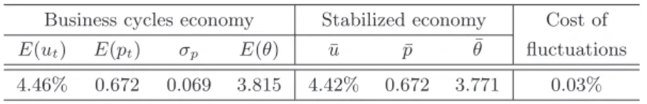
Table 4: The welfare cost of fluctuations in a matching model with rigid wages
Business cycles economy Stabilized economy Cost of
E(ut) E(pt) σp E(θ) u¯ p¯ θ¯ fluctuations
α = 0.5 10.22% 0.285 0.069 0.72 9.82% 0.285 0.681 0.44%
α = 0.4 10.22% 0.285 0.069 0.72 9.75% 0.288 0.678 0.55%
α = 0.6 10.22% 0.285 0.069 0.72 9.89% 0.283 0.685 0.32%
Table 4, Line 1, presents the results for the benchmark calibration of the rigid wage model. These results show that the average unemployment rate is higher in the fluctuating economy. This is also the case for the average labor market tightness, and so for the average vacancies as well. As expected, there is no influence of productivity fluctuations on the average job finding rate as α = 0.5, and the welfare cost of business cycles is of the same magnitude as in the reduced form analysis33. The size of the business cycle cost is only determined by the u-convexity effect.
32As noted before, Hall [2005] uses a measure of unemployment expanded to include “discouraged workers”
and “marginally attached workers”. As workers are considered to be homogenous in our model, we then assume that “discouraged workers” generate the same surplus from working as the workers who are officially unemployed, which is debatable. If the surplus was lower, the business cycle costs would also be lower.
33Note that the cost-decreasing effect of the covariance between productivity and employment, offset by the
cost-increasing effect of higher vacancies, generates a small change in the business cycle costs relative to the employment loss (less than 0.06 of a percentage point compared to 0.44).
We then simulate two other cases: α = 0.4 and α = 0.6 (last two lines of Table 4). The values of the parameters κ,γ and ϕ have been changed accordingly in order to still match the job finding rate characteristics34. Depending on α, the US welfare cost of fluctuations could reach 0.55%
or reduce to 0.32%. Petrongolo and Pissarides (2001) estimate this elasticity to be between 0.3 and 0.5. This suggests that with α = 0.5, our benchmark calibration gives a lower bound of the welfare costs of fluctuations. In the more realistic case (α = 0.4), the average job finding rate in the fluctuating economy is lower than the value which would be reached in the stabilized economy. A lower elasticity strengthens the p-concavity effect and dampens the θ-convexity effect. In this case, the internal mechanism of the matching model leads to quite high business cycle costs, since these costs are increased by one fourth. Note that it occurs only when the labor market tightness θ (and so the job finding rate p(θ)) is volatile enough to make the non-linearity operate. Replicating the volatility of both the labor market tightness and the job finding rate leads to sizable business cycle costs through different channels which are all at work in this structural model.
We believe that these results are quite general and do not depend on the rigid wage framework we consider here35. Firstly, the business cycle costs are mainly generated by the u-convexity,
which is a key feature of any matching model. Secondly, the non-linearity of the job finding rate due to the matching function is not specific to the rigid wage economy. The flexible wage case actually adds other sources of non-linearity which depend on the specification of the matching model considered. The next section explicitly addresses this robustness issue.
4
Robustness
In this section, we evaluate the robustness of our results by undertaking two very different strate-gies. Firstly, we consider the alternative view to the rigid-wage approach proposed by Hagedorn and Manovskii (2008). Secondly, we propose to test the presence of a convex relationship be-tween productivity shocks and unemployment through a cross-country panel analysis.
4.1 A flexible-wage approach
Hagedorn and Manovskii (2008) have recently proposed an alternative response to the Shimer puzzle by suggesting that the problem is more in the way the model is calibrated than in the
34Note that, in the α = 0.4 case, the rigid wage defined at the median productivity is no longer in the bargaining
set. The wage is then fixed at its highest value ensuring that the firm’s value is still positive (w = argminyπy).
35Our result suggests another interpretation to the cost of the wage rigidity given by Shimer (2004). This cost
is of the same order of magnitude as our measure. He interprets this cost as the result of the non-optimality of the labor market tightness volatility. Our result rather suggests that it comes from the employment loss generated by the volatility of the job finding rate. Note that Shimer (2004) indeed emphasizes that the average output in the rigid wage economy is 0.12 percent below the level in the flexible wage one.
model itself. The matching framework with flexible wages can generate a realistic volatility in the job finding rate when the value of unemployment and of the workers’ bargaining power are judiciously calibrated. Considering this alternative view enables us to qualify our results. In this flexible wage framework, the welfare cost of business cycles may differ from the results derived under rigid wages for several reasons. Firstly, the non linearity in the job finding rate is modified due to the retroaction of wages in the job creation condition. Appendix E indeed shows that the condition which ensures that the job finding rate is lowered by business cycles is less stringent in this flexible wage environment. For the same value of α, the flexible wage framework potentially leads to higher business cycle costs. Secondly, the employment loss is no longer necessarily a good approximation of the welfare cost of business cycles. The covariance between productivity and employment and the behavior of vacancies over the cycle matter for the size of the market production loss (equation (14)). Further, the calibration of Hagedorn and Manovskii (2008) adds another difference: they show that the volatility of the job finding rate is high enough only if the value of the non-market activity z is calibrated sufficiently close to the average productivity. This implies calibrating z at a much higher value than its strict interpretation as an unemployment benefit would imply. Following Hagedorn and Manovskii (2008), we consider that z now includes home production l. It leads to a redefinition of aggregate consumption as follows: c = y(1 − u) + ul − κv. It implies that the business cycle welfare cost is different from the market production loss defined in equation (14) and is then sensitive to the value of l:
λl≈ (E(u) − ¯u)(1 − l) − cov(y, 1 − u) + κ(E(v) − ¯E(c) v) (27)
Let us emphasize that, for a given level of z, the value of l matters only for the magnitude of the welfare costs and has no effect on average employment and vacancy rates.
In order to check the robustness of our results, we now calibrate the flexible wage equilibrium, defined by the equations (9), (11) (20) and (21), along the lines of Hagedorn and Manovskii (2008). We consider the same values as in our benchmark economy for all parameters, except for the workers’ bargaining power γ, the non-market value z and the vacancy cost κ which are calibrated in order to match the same targets as in the rigid wage case for internal consistency36.
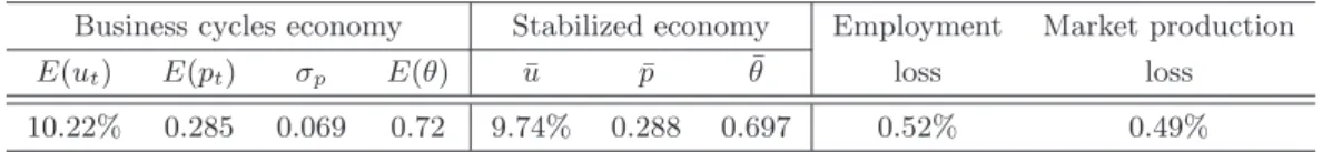
Table 5: Employment and market production loss with flexible wages
Business cycles economy Stabilized economy Employment Market production
E(ut) E(pt) σp E(θ) ¯u p¯ θ¯ loss loss 10.22% 0.285 0.069 0.72 9.74% 0.288 0.697 0.52% 0.49%
Table 5 shows that the effects of the non-linearities present in the matching model appear to
36Note that the targets are different in Hagedorn and Manovskii (2008). The values of κ, γ and z are respectively
be quite robust to variations in the degree of wage rigidity. The employment loss is even larger than in the rigid wage approach (0.52% against 0.44% in Table 4), as the stabilized job finding rate is now higher than its cyclical counterpart for α equal to 0.5. For the calibration considered in this flexible wage framework, the threshold for α under which the job finding rate is higher in the stabilized economy is 0.63 (vs. 0.5 in the rigid wage economy)37. However, as wages are now flexible, this employment loss does not necessarily coincide with the market production loss. Actually, the last column in Table 5 shows that these two losses are very close. The interaction between productivity and employment is nearly compensated by the the vacancy gain. This result is not surprising: as the calibration is such that the bargained wage is close to the constant outside opportunity of the employed workers, this flexible wage model “is a close cousin of others that rationalize wage rigidity by dropping Nash wage bargaining” (Hall (2006), p.16).
However, the extent to which the employment (or the market production) loss can be interpreted as a welfare cost crucially depends on the home production value l. The standard calibration of the unemployment benefits for the US economy is between 0.3 and 0.6 (Kitao et al. (2008), Nickell et al. (2005) and Shimer (2005)). For the calibrated value of 0.97 for z, this implies that l is between 0.37 and 0.67, leading to a welfare cost equal to 0.30% and 0.14% respectively. Obviously, a high value of l automatically lowers the costs of business cycles. This question of the value of non-market activities is undoubtedly key for the welfare costs of business cycles. Let us emphasize that our results on the employment loss are robust to considering flexible wages. We believe they would also be robust to other matching models solving the Shimer puzzle as the underlying mechanisms are intrinsic to this class of models38. On the other hand, our results on
the welfare costs are sensitive to the home production value, but this value remains so highly debated among the profession that we consider that this is more a matter of opinion than a matter of fact. Furthermore, when non-market returns are high, the response of unemployment to unemployment insurance is too large (Costain and Reiter (2008)). Hall and Milgrom (2008) also noted that the Hagedorn and Manovskii calibrations imply too high a labor supply elasticity, given empirical estimates.
Moreover, it must be emphasized that we have neglected other dimensions that could have increased our quantitative measure of the business cycle welfare costs. Once the non-market production is considered to be as efficient as the market production, the disutility of “not working” may dominate the disutility of working when job search costs, as well as indirect costs such as psychological damage and skill obsolescence, are taken into account. There are no clear empirical answers on this crucial point. On the other hand, unemployment benefits do not lead to distortive taxation in our theoretical framework. Business cycles, by increasing average
37See Appendix E.
38In Hairault et al. (2008), we show that this is true in the case of the fixed cost of recruiting recently introduced
unemployment, could imply higher taxes, which would, in turn, weigh employment down. This could have been counted as a cost of business cycles. Another dimension which could magnify these costs is the loss of human capital generated by unemployment spells and reflected in the permanent decrease in wages observed in data (Krebs (2007), Jung and Kuester (2008)). Is this compensated for by more intense human capital accumulation during expansions? All these points would deserve to be addressed to obtain a more general assessment of the welfare cost of unemployment fluctuations.
4.2 Unemployment and non-linearity: a test on panel data
The cost of business cycles induced by matching frictions relies crucially on the convexity between unemployment and total factor productivity. In this section, empirical estimates of this effect, based on cross-country data, are provided39. Equation (25) can be used as a guideline to gauge
whether more volatility is associated with substantially higher unemployment after controlling for other determinants of unemployment.
We use the panel data constructed by Bassanini and Duval (2006) over the period 1982-2003 for 20 OECD countries40, which provide the unemployment rate (consistent with Shimer data), the
cyclical component of the total factor productivity process (tfp) and time-varying labor market institutions (LMI) indicators for each country. The LMI aim at accounting for the structural level of unemployment. They include the average unemployment benefit replacement rate, the tax wedge, an indicator of employment protection legislation, an indicator of product market regulation, an indicator of high corporatism in the wage bargaining process and the union density41. In order to test whether the relation between the unemployment rate and the total
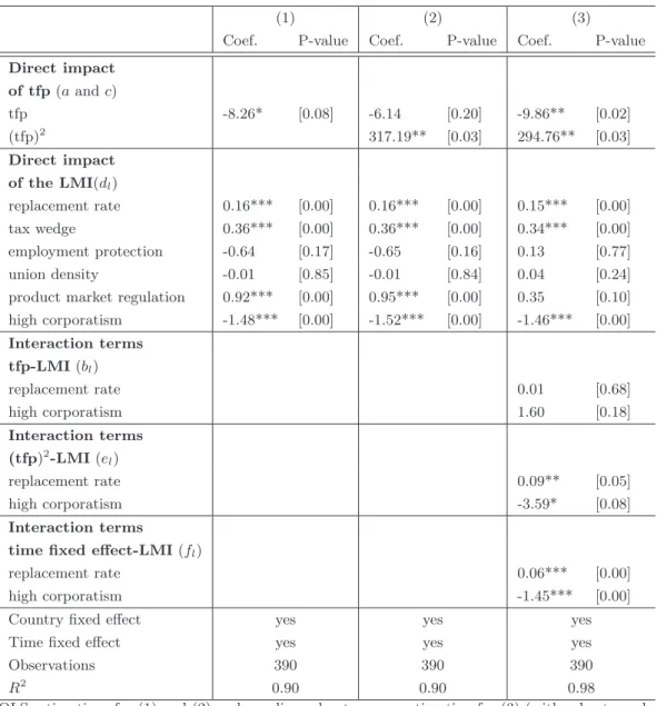
factor productivity is convex, we augment the standard specification of Bassanini and Duval (2006) by introducing the square of the tfp:
ui,t=
X
l
dlXi,tl + a tfpi,t+ c (tfpi,t)2+ γi+ λt+ ²i,t (28)
where Xl
i,tdenotes the LMI l in country i at time t, λtthe time fixed effect and γi is the country
fixed effect. The results of this specification are shown in Column (1) and (2) of Table 6. We then include a possible interaction42between tfp and time-invariant LMI, consistently with
equation (25). Indeed, besides their direct effects on the structural unemployment, LMI may affect the impact of tfp on unemployment. Furthermore, as the non-linearity too may depend
39We thank one referee for suggesting this empirical exercise.
40Observations for Finland, Germany and Sweden in 1990 and 1991 are removed from the sample as in Bassanini
and Duval (2006). We drop New Zealand and Portugal because there are a lot of missing values in the shock series for these two countries.
41See Appendix 2 in Bassanini and Duval (2006) for a detailed description of the variables. 42We also allow the time fixed effect (λ