Visible Light Range-Finding and Communication Using the Automotive LED Lighting

(1)

HAL Id: tel-01685450

https://hal.archives-ouvertes.fr/tel-01685450

Submitted on 16 Jan 2018

HAL is a multi-disciplinary open access archive for the deposit and dissemination of sci-entific research documents, whether they are pub-lished or not. The documents may come from teaching and research institutions in France or abroad, or from public or private research centers.

L’archive ouverte pluridisciplinaire HAL, est destinée au dépôt et à la diffusion de documents scientifiques de niveau recherche, publiés ou non, émanant des établissements d’enseignement et de recherche français ou étrangers, des laboratoires publics ou privés.

the Automotive LED Lighting

Bastien Béchadergue

To cite this version:

Bastien Béchadergue. Visible Light Range-Finding and Communication Using the Automotive LED Lighting. Signal and Image processing. Université Paris Saclay, 2017. English. �tel-01685450�

(2)

Mesure de distance et

transmission de données

inter-véhicules par phares à LED

Thèse de doctorat de l'Université Paris-Saclay

préparée à l’Université de Versailles

Saint-Quentin-en-Yvelines

École doctorale n°580

Sciences et Technologies de l’Information et de la

Communication (STIC)

Spécialité de doctorat: Traitement du signal et des images

Thèse présentée et soutenue à Vélizy-Villacoublay, le 10 novembre 2017, par

Bastien Béchadergue

Composition du Jury : Mme. Véronique Vèque

Professeure, Université Paris-Sud (L2S) Présidente

Mme. Anne Julien-Vergonjanne

Professeure, Université de Limoge (XLIM) Rapportrice

M. Thierry Bosch

Professeur, INP de Toulouse (LAAS) Rapporteur

M. Dominic O’Brien

Professeur, Université d’Oxford Examinateur

M. Fawzi Nashashibi

Directeur de recherche, INRIA (RITS) Examinateur

M. Luc Chassagne

Professeur, Université Paris-Saclay, UVSQ (LISV) Directeur de thèse

M. Hongyu Guan

Ingénieur de recherche, Université Paris-Saclay, UVSQ (LISV) Co-Directeur de thèse

M. Jean-Laurent Franchineau

Directeur de programme, Institut Vedecom Invité

NNT

:

2

0

1

7 S

A

CL

V

0

85

(3)

(4)

Université Paris-Saclay

Espace Technologique / Immeuble Discovery

Route de l’Orme aux Merisiers RD 128 / 91190 Saint-Aubin, France

Titre : Mesure de distance et transmission de données inter-véhicules par phares à LED Mots clés : communication optique sans fil, mesure de distance, véhicule autonome, LiFi

Résumé : En réponse aux problèmes croissants liés aux transports routiers - accidents, pollutions, congestions - les véhicules à faibles émissions, équipés de systèmes de transports intelligents (ITS) sont progressivement développés. Si la finalité de cette démarche est le véhicule entièrement autonome, on peut néanmoins s'attendre à voir d'abord sur nos routes des véhicules automatisés sur des phases de conduite spécifiques. C'est le cas du convoi automatisé, qui permet à plusieurs véhicules de rouler en convois de manière automatique et donc d'augmenter la capacité des voies de circulation tout en réduisant la consommation de carburant. La fiabilité de cet ITS repose sur plusieurs briques technologiques, et en particulier sur la mesure de distance et la transmission de données véhicule-véhicule (V2V).

De nombreux systèmes permettent de réaliser ces deux fonctions vitales comme, par exemple, les radars ou lidars pour la mesure de distance et la technologie IEEE 802.11p pour la communication véhiculaire. Si ces différents dispositifs présentent de très bonnes performances, ils sont néanmoins particulièrement sensibles aux interférences, qui ne cessent de se multiplier à mesure que le nombre de véhicules équipés augmente et que le trafic est dense. Pour pallier les dégradations de performances induites par de telles situations, des technologies complémentaires pourraient donc être utiles. Le récent développement des diodes électroluminescentes (LED) blanches, en particulier pour l'éclairage automobile, a permis l'émergence des communications optiques visibles sans fil (VLC). Les phares à LED sont alors utilisés pour transmettre des données entre véhicules et avec les infrastructures. Malgré la puissance limitée de ces éclairages, plusieurs études ont montré qu'une transmission de qualité est possible sur quelques dizaines de mètres, faisant de la VLC un complément particulièrement intéressant à l'IEEE 802.11p, en particulier pour les convois automatisés. Par analogie, on peut alors se demander si les phares ne pourraient pas être aussi utilisés pour mesurer la distance V2V.

Le but de cette thèse est donc de proposer et évaluer un système dédié aux situations de convois automatisés qui, à partir des phares avant et arrière des véhicules, transmet des données et mesure simultanément la distance V2V. Dans un premier temps, une étude détaillée de l'état de l'art de la VLC pour la communication V2V est effectuée afin de déterminer l'architecture de base de notre système. La fonction de mesure de distance est ensuite ajoutée, après une revue des différentes techniques usuelles. Une fois l'architecture générale du système établie, elle est dans un premier temps validée par des simulations avec le logiciel Simulink. En particulier, les différents paramètres sont étudiés afin de déterminer leur impact sur la résolution de mesure de distance et les performances en transmission de données, puis afin de les optimiser. Si ces simulations fournissent des indicateurs importants pour la compréhension du système, elles ne peuvent cependant remplacer les tests d'un prototype réel. L'implémentation de ce prototype est alors détaillée ainsi que les tests réalisés dans différentes configurations. Ces différents tests démontrent l'intérêt des solutions proposées pour la mesure de distance et la communication V2V en convois automatisés.

(5)

Université Paris-Saclay

Espace Technologique / Immeuble Discovery

Route de l’Orme aux Merisiers RD 128 / 91190 Saint-Aubin, France

Title: Visible Light Range-Finding and Communication Using the Automotive LED Lighting Keywords: visible light communication, distance measurement, autonomous vehicle

Abstract : In response to the growing issues induced by road traffic - accidents, pollution, congestion - low-carbon vehicles equipped with intelligent transportation systems (ITS) are being developed. Although the final goal is full autonomy, the vehicles of the near future will most probably be self-driving in certain phases only, as in platooning. Platooning allows several vehicles to move automatically in platoons and thus to increase road capacity while reducing fuel consumption. The reliability of this ITS is based on several core technologies and in particular on vehicle-to-vehicle (V2V) distance measurement and data transmission.

These two vital functions can be implemented with several kinds of systems as, for instance, radars or lidars for range-finding and IEEE 802.11p-based devices for vehicular communication. Although these systems provide good performances, they are very sensitive to interferences, which may be a growing issue as the number of vehicles equipped will increase, especially in dense traffic scenario. In order to mitigate the performance degradation occurring in such situations, complementary solutions may be useful. The recent developments of white light-emitting diodes (LED), especially for the automotive lighting, has allowed the emergence of visible light communication (VLC). With VLC, the vehicle headlamps and taillights are used to transmit data to other vehicles or infrastructures. Despite the limited optical power available, several studies have shown that communication over tens of meters are possible with a low bit error rate (BER). VLC could thus be an interesting complement to IEEE 802.11p, especially in platooning applications. By analogy, one could wonder if the automotive lighting can also be used for V2V range-finding.

The goal of this thesis is thus to propose and evaluate a system dedicated to platooning configurations that can perform simultaneously the V2V distance measurement and data transmission functions using the headlamps and taillights of the vehicles. The first step of this study is thus a detailed state-of-the art on VLC for V2V communication that will lead to a first basic architecture of our system. Then, the range-finding function is added, after a careful review of the classical techniques. Once the general architecture of the system is drawn, it is validated through simulations in the Simulink environment. The different degrees of freedom in the system design are especially studied, in order first to evaluate their impact on the measurement resolution and the communication performances, and then to be optimized. Although these simulations provide crucial keys to understand the system, they cannot replace real prototype testing. The implementation of the prototype is thus fully described, along with the results of the different experiments carried out. It is finally demonstrated that the proposed solution has a clear interest for V2V range-finding and communication in platooning applications.

(6)

(7)

(8)

Remerciements

Les travaux ici présentés sont le fruit de mes trois années de thèse au Laboratoire d’Ingénierie des Systèmes de Versailles de l’Université de Versailles Saint-Quentin-en-Yvelines et à l’Institut Vedecom. Je remercie donc tout d’abord Luc Chassagne, directeur du laboratoire, et Jean-Laurent Franchineau, directeur du programme Eco-Mobilité de Vedecom, de m’avoir donné la chance de réaliser ce doctorat.

Cette thèse a été réalisée sous la direction de Luc Chassagne, que je tiens de nouveau à remercier chaleureusement, pour son suivi constant et bienveillant ainsi que pour ses précieux conseils qui m’ont aiguillé tout au long de mon parcours de doctorant. Elle a par ailleurs été co-encadrée par Hongyu Guan, que je remercie vivement pour toutes ses remarques constructives.

Tous mes remerciements vont également à Mme. Anne Julien-Vergonjanne et M. Thierry Bosch, pour l’intérêt qu’ils ont porté à mon travail en acceptant d’en être les rapporteurs, à Mme. Véronique Vèque pour avoir présidé le jury de soutenance et à M. Dominic O’Brien et M. Fawzi Nashashibi qui ont accepté d’être dans mon jury.

Ces travaux n’auraient sans doute pas abouti sans le concours d’Olivier, de ses fléchettes, et plus généralement de tous les membres du laboratoire qui contribuent chaque jour à en faire un lieu chaleureux et stimulant pour mener des recherches. Mes pensées vont en particulier à mes chers collègues du troisième étage que je remercie infiniment pour leur disponibilité et leur bonne humeur constante. De même, je remer-cie l’encadrement de Vedecom, en commençant par Samir Tohmé, pour l’autonomie qui m’a été accordée, ainsi que tous les collègues que j’ai pu côtoyer lors de mes trop rares passages et en particulier les membres de l’équipe MOB01.

J’ai eu la chance durant cette dernière année de thèse d’effectuer un séjour de recherche de deux mois à Taïwan. Je tiens donc à remercier le Ministère des Sciences et Tech-nologies de Taïwan et la National Taiwan University de m’avoir permis de vivre cette expérience unique. Je remercie également Hsin-Mu Tsai, qui m’a accueilli et supervisé durant ce séjour, ainsi que tous les membres de son laboratoire et de l’IoX Center pour leur sympathie. Je ne peux refermer cette parenthèse taïwanaise sans avoir une pensée pour mes camarades de voyage, en particulier Stephanie, Adrien, Romain, Chun-Ju...

Ces trois années ont été marquées par des moments d’allégresse, d’incertitude et parfois de tristesse. J’ai une pensée émue pour mon cher ordinateur portable, qui après des années de bons et loyaux services, a décidé de rendre l’âme quelques jours avant ma soutenance. Mais je remercie surtout mes amis, grâce à qui j’ai pu mettre de côté mes tracas de thésard, en commençant par les plus anciens, Anouk, François et Sylvain, et avec une pensée spéciale pour Emma et Boubou. Je pense aussi à mes camarades d’aviron, qui m’ont rappelé chaque semaine qu’il y avait des choses bien

(9)

Enfin, et surtout, je remercie profondément ma famille, qui a toujours été présente pour moi et m’a constamment soutenu dans mes choix.

(10)

List of Figures

1.1 (a) Growth of the vehicle fleet in EU 17 in millions of units [3], (b) passenger and goods transport growth in EU 28 [4]. . . 2

1.2 Past and potential future evolution toward automated cooperative driving [7].. . . 4

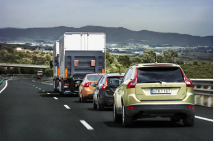
1.3 Illustration of the concept of platooning, here with the SARTRE project. 7

1.4 Detail of (a) the DSRC layers [14] and (b) the C-ITS layers [15]. . . . 9

1.5 Different characteristics of lidar, radar, ultrasonic and passive visual (camera) sensors [18]. . . 10

1.6 Range-finding and data transmission requirements for highway pla-tooning applications. . . 12

2.1 Optical beacons used in VICS [21]. . . 17

2.2 Evolution over the years of the number of academic publications ref-erenced by the IEEE Xplore Digital Library when searching the term ‘Visible Light Communication’. . . 19

2.3 General architecture of a VLC system. . . 19

2.4 (a) Package of a ‘Superflux’ red LED commonly used for automotive back lighting and (b) corresponding transmission beam pattern [30]. . 20

2.5 Relative spectral sensitivity of a photodiode against (a) the wave-lengths and (b) the angular displacement [31].. . . 21

2.6 The different VLC link configurations [23].. . . 22

2.7 Block diagram of the I2V-VLC (a) emitter and (b) receiver proposed by Hochstein in [38]. . . 26

2.8 Illustration of the camera optical channel behavior with images of the traffic light captured (a) at short distance and (b) at log distance [48]. 27

2.9 User interface of the camera-based V2V-VLC system detailed in [63]. . 30

2.10 Transimpedance amplifier stage with (a) an ideal photodiode and (b) the equivalent model of a real photodiode. . . 31

2.11 Detailed design of the VLC receiver used in [68]. . . 33

2.12 Detailed view of the OCI sensor [63]. . . 35

2.13 Block diagram of the VLC prototype for scooter-to-scooter communi-cation [80]. . . 36

2.14 General design of the VLC function of the VLCR. . . 38

(17)

2.16 (a) Current-voltage characteristics of the headlamps used in the pro-totypes and (b) evolution of their maximum luminous intensity with the forward current. . . 41

2.17 Spatial distribution of the luminous intensity of a headlamp driven by a current of 600 mA, when projected on a vertical plane at 4.5 m. The point of origin is the point of maximum luminous intensity 50 L. . . . 42

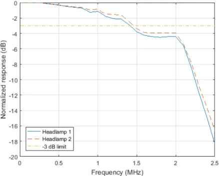
2.18 Frequency responses of both headlamps with the -3 dB limit. . . 42

2.19 Current-voltage characteristic of the COTS taillights when (a) in stop mode and (c) in traffic mode, evolution of their maximum luminous intensity with the forward voltage when (b) in stop mode and (d) in traffic mode.. . . 43

2.20 Spatial distribution of the luminous intensity of a taillight when pro-jected on a vertical plane at 1 m in (a) traffic mode and (b) stop mode. 44

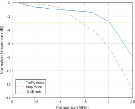
2.21 Frequency responses of the taillights in traffic mode (plain blue line) and stop mode (dashed red curve), with the -3 dB limit (yellow dashed dots). . . 45

2.22 LiFi modulation techniques tree [91]. . . 46

2.23 Frequency spectrum of an OOK data signal at f_c = 2 MHz, with (a) no additional coding and (b) Manchester coding. . . 47

2.24 Modulation of the data frame 01101100 in OOK, PAM-4 and GSSK with Manchester coding according to the clock signal of rate fc.. . . . 49

2.25 Block diagram of the boomerang system [110]. . . 51

2.26 Illustration of the concept of (a) passive reflection and (b) active re-flection. . . 52

3.1 Working principles of triangulation, with α, β and Φ the angles of emission, δ, γ and ψ the angles of incidence and d the distance between the emitter and the receiver [126]. . . 57

3.2 Geometrical principles of the automotive triangulation rangefinder pro-posed in [127]. . . 57

3.3 Principles of the positioning rangefinder based on the automotive light-ing proposed in [128], with τ_i the propagation delays from both emit-ters, separated by a distance LA, to both receivers, separated by a

distance L_B.. . . 58

3.4 Principles of FMCW range-finding. The signal sent Er is modulated

with a linear frequency modulation of depth ∆f and the echo received

Em contains a frequency shift fif proportional to the distance d. . . . 59

3.5 Different types of automotive radars with their respective characteris-tics [130]. . . 60

(18)

3.7 Principles of pulsed TOF distance measurement with light. A signal

E(t) is sent and the echo, reflected by a target at distance D, is received

with a proportional delay ∆t [138]. . . . 62

3.8 Working principles of a TOF 3D camera rangefinder [140]. . . 64

3.9 Design of the automotive laser phase-shift rangefinder proposed in [145]. 66

3.10 (a) Block diagram of the auto-digital phase measurement technique and (b) chronogram illustrating its functioning. . . 69

3.11 Heterodyning of a signal se by undersampling with a synchronized

clock s_h when r = 10. . . . 70

3.12 Block diagram of the VLCR. . . 72

3.13 Block diagram of the VLR. . . 74

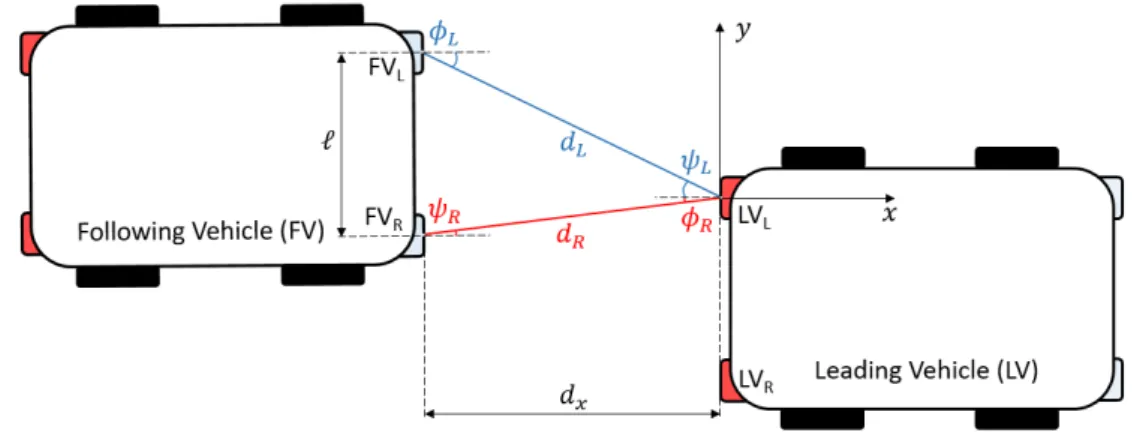
3.14 Set-up of the general positioning VLCR, with dx, φx and ψx denoting

the different distances, irradiance angles and incidence angles. . . 75

3.15 Set-up of the straight line positioning VLCR, with dx, φx and ψx

de-noting the different distances, irradiance angles and incidence angles. . 76

3.16 Evolution of the count-induced distance error with the counting fre-quency fclock and the intermediate frequency fi, whatever the

hetero-dyning method used. . . 78

3.17 Heterodyning of a signal srby undersampling with a non-synchronized

clock s_h when r = 10. . . . 79

3.18 Illustration of the production of two phase-shift pulses with an hetero-dyning of factor r = 10. . . . 80

3.19 Geometry of a platoon in a straight line configuration. . . 81

3.20 Evolution of (a) the maximum static error δd_m,het induced by the het-erodyning step and (b) the intermediate frequency fi with the

hetero-dyning factor r and the frequency of operation fe. . . 83

4.1 Geometry used for the channel gain derivation, with θ and φ the polar and azimuth angles of emission, ψ the angle of incidence, Ar the PD

area, A_{ef f} the effective PD area seen from the transmitter and d the distance from the transmitter to the receiver. . . 88

4.2 Two-vehicles platoon of inter-distance d, in a curve of center C and radius R and fully defined by the angle α. . . . 92

4.3 Simulink model of the VLR. . . 93

4.4 Details on the signal reconstruction blocks ‘Rx LV’ and ‘Rx FV’ of the VLR.. . . 94

4.5 Evolution with the distance of the SNR at the receiver level and in the reference axis of the transmitter when the latter is a headlamp (plain blue line) or a taillight (red dashes). . . 95

(19)

4.6 (a) Square signal se transmitted at 1 MHz, (b) signal sp0 produced by the front-end stage of the receiver with an SNR = 3 dB, before processing and (c) after filtering with 4th order Butterworth filters of respective low-pass cut-off frequency 1.05 MHz and high-pass cut-off frequency 950 kHz, (d) square signal s_r0 reconstructed by zero-crossing detection. . . 96

4.7 Evolution with the SNR of the similarity between the transmitted and reconstructed square signals se and sr0 for different orders of the re-construction filters. . . 97

4.8 Evolution of the distance measured by an ideal VLR when operating at f_e = 1 MHz with an heterodyning factor r = 3999 over a range going from 5 m to 150 m by steps of 1 m. . . 100

4.9 Evolution of the distance measured by an ideal VLR for various het-erodyning factors r and frequencies of operation fe.. . . 101

4.10 Evolution with the real distance, in the central case (‘Case 1’) and by steps if 1 cm, of the distance measured by the VLR (blue line) with its linear fit (red dashes) and of the real distance (black dots). . . 102

4.11 Evolution, by steps of 1 cm, of the distance measurement error against the real distance before correction for the central case (‘Case 1’). . . . 103

4.12 Histogram of the distance measurement error after correction over the range going from 5 m to 30 m (blue blocks) and its Gaussian fit (red curve) in the central case (‘Case 1’). . . 103

4.13 (a) Part of the signal sp produced by the PD of the FV while the V2V

distance is 50 m, (b) signal obtained after band-pass filtering and (c) signal reconstructed sr. . . 104

4.14 Evolution, by steps if 1 cm, of the distance measured by the VLR against the real distance for different orders of filters (a) before cor-rection and (b) after corcor-rection over then range going from 5 m to 30 m. . . 107

4.15 Evolution, by steps if 1 cm, of the distance measured against the real distance with various heterodyning factors r. . . . 108

4.16 Evolution, by steps if 1 cm, of the distance measured against the real distance with various frequencies of operation f_e. . . 110

4.17 Histogram of the distance measurement error after correction (blue blocks) and its Gaussian fit (red curve) in the case of a frequency of operation f_e= 4 MHz (‘Case 5’). . . 110

4.18 (a) Time evolution of the distance measured by the VLR (blue line) and of the actual distance (red dashes) while the FV is moving toward the LV at v0 = 20 km/h from an initial distance of 15 m and (b) histogram of the resulting measurement error (blue blocks) with its Gaussian fit (red line). . . 112

(20)

4.19 Evolution, by steps of 1 cm, of the lateral and longitudinal coordinates

xFVL and yFVL of the point FVL estimated by the VLR and of their true values. . . 114

4.20 Histogram of the error (blue blocks) in (a) longitudinal coordinate x_FV_L and (b) the lateral coordinate y_FV_L with its Gaussian fit (red curve). . 115

4.21 Block diagram of the Simulink model for the VLCR. . . 117

4.22 (a) Data signal transmitted m_e0, (b) signal received m_p with AWGN of SNR = 3 dB, before processing and (c) after filtering with two 2nd order Butterworth filters of respectively low-pass cut-off frequency 500 kHz and high-pass cut-off frequency 5 kHz (blue curve) and hysteresis triggering (dotted and plain red lines), (d) signal d_r reconstructed by triggering. . . 119

4.23 Cross-correlation between a transmitted binary message and its recon-structed version after ‘VLC filtering’. . . 120

4.24 (a) Data signal transmitted me0, (b) signal received m_p with AWGN of SNR = 3 dB, before processing and (c) after filtering with two 2nd order Butterworth filters of respectively low-pass cut-off frequency 2.5 MHz and high-pass cut-off frequency 250 kHz (blue curve) and hystere-sis triggering (dashed and plain red lines), (d) signal dr reconstructed

by triggering. . . 121

4.25 Cross-correlation between a transmitted binary message and its recon-structed version after (a) ‘VLC filtering’ and (b) ‘VLR filtering’. . . . 122

4.26 BER and PER evolution against the inter-vehicle distance by steps of 50 cm and combination of ‘VLC filtering’ (VLC_f) or ‘VLR filtering’ (VLR_f) with pulse width decoding (PW_d) or clock decoding (C_d). . . 124

4.27 (a) Signal mp0 received by the LV from a distance of 40 m, (b) signal filtered by ‘VLR filtering’ and (c) signal reconstructed d_r0. . . 124 4.28 Distribution of the pulse width count values when the V2V distance is

(a) 25 m and (b) 75 m.. . . 126

4.29 (a) Evolution, against the real distance (black dotted line), of the esti-mated distance using ‘VLR filtering’ (red dashes) and ‘VLC filtering’ (blue curve), (b) histogram of the error after correction over the range 1 m to 30 m in the case of ‘VLR filtering’ with its Gaussian fit curve. 127

5.1 Typical MOSFET driver for LED. . . 133

5.2 Light signals, observed with a Thorlabs PDA8A, produced by the head-lamps and taillights when driven by a square wave of frequency (a) 100 kHz and (b) 1 MHz. . . 134

5.3 Frequency response of the custom-made front-end (blue line) with the -3 dB limit (red dashes). . . 136

5.4 Block diagram of the processing chain used for VLC signal reception and reconstruction. . . 136

(21)

5.5 Time evolution of a data signal 100110 transmitted from 10 m at 100 kbps with a single taillight in traffic mode after (a) reception by the front-end stage, (b) band-pass filtering of low-pass and high-pass cut-off frequencies of respectively 100 kHz and 1 kHz, (c) amplification and (d) zero-crossing detection. . . 137

5.6 Distribution of the count values obtained with pulse width decoding in the offline mode, with a sampling rate equal to 12.5f_c, on packets started by the header H = 1111. . . . 139

5.7 Emitter and receiver structures used for the VLC experiments. . . 139

5.8 OOK data signal at 100 kbps digitized in the case of F2L communica-tion at 30 m. . . 141

5.9 (a) OOK data signal at 100 kbps digitized in the case of L2F commu-nication with taillights in traffic mode at 10 m, (b) histogram of the pulse width values when d = 12 m. . . . 142

5.10 Example of transmission latency at 100 kbps, measured as the time between the first rising edge of the message (in orange) and the rising edge of the enable bit (in blue). . . 144

5.11 Set-up used to investigate the impact of the interferences generated by other vehicles, in both the F2L vehicle communication and L2F vehicle communications cases. . . 145

5.12 Evolution with the longitudinal distance of the contribution of the jamming light signal in the total illuminance perceived at the receiver level when the lateral distance is 2 m. . . 146

5.13 Block diagram of the VLC system operating at 100 kbps used in dy-namic tests [172]. . . 148

5.14 Optical system placed in front of the Thorlabs PDA100A to enhance the optical power received [172]. . . 149

5.15 General view of the set-up used for the tests in real driving conditions [172].. . . 150

5.16 (a) 18 km freeway segment along which the vehicles have been driven and (b) view of the V2V configuration provided by the Mio Combo 5107 [172]. . . 151

5.17 Time evolution of the BER, calculated every 10000 consecutive bits (black peaks), and of the longitudinal V2V distance (orange curve). . 152

5.18 Spatial distribution of the PRR at 100 kbps. The point of origin is the location of the FV whereas the points on the grid are the different positions of the LV.. . . 152

5.19 Examples of PAM-4 data signal at 200 kbps detected by one of the re-ceivers when the V2V distance is 30 m, with its decoding zones defined by the black horizontal lines. . . 155

(22)

5.20 Left column: GSSK signals at 200 kbps sampled by the left receiver (blue line) and the right receiver (orange dashes) when the V2V dis-tance is (a) 5 m, (b) 10m and (c) 30 m. Right column: Lateral evo-lution, at the receivers level, of the illuminance produced by the left headlamp (blue dotted dashes), the right headlamp (red dotted plain line) and both headlamps (orange line) when the V2V distance is (d) 5 m, (e) 10 m and (f) 30 m. . . 156

5.21 Example of GSSK data signals at 200 kbps sampled by the left receiver (blue line) and the right receiver (orange dashes) when the FV/LV distance is d = 10 m and the radius of the curve is R = 100 m. . . . . 158

5.22 Emitter and receiver structures used for the VLC experiments with large clock rates. . . 159

5.23 Example of (a) OOK data signal with f_c = 2 MHz, (b) PAM-4 data signals with fc= 200 kHz (blue line), fc= 500 kHz (red dashes), fc= 1

MHz (yellow dots-dashes) and fc= 2 MHz (purple dots) and (c) GSSK

data signals of the left (blue line) and right (red dashed line) receivers, with fc= 2 MHz. In (b), signals are time scaled to ease comparison. . 161

5.24 Comparison of the characteristics of OOK, PAM-4 and GSSK accord-ing to their data rate, simplicity of implementation and robustness to mobility, for a BER below 10−6, in highway platooning configurations. 163

5.25 Illustration of the processing chain of the VLR: in yellow, input signal of peak-to-peak amplitude 20 mV_pp and SNR = 5 dB, in purple, its FFT, in pink, signal obtained after band-pass filtering and in blue square signal reconstructed by the high-speed comparator. . . 166

5.26 Details of the reconstructed sine wave (in pink) and square wave (in blue) when the input signal (in yellow) is noiseless. . . 166

5.27 Evolution of the average phase-shift measured by the dedicated FPGA algorithm with an heterodyning factors r = 3950.007. . . 168

5.28 Distribution of the measurement error induced by FPGA implementa-tion of the auto-digital phase measurement algorithm. . . 168

5.29 Detail on the evolution of the average phase-shift measured by the dedicated FPGA algorithm with an heterodyning factors r = 3950.007. 169

5.30 Set-up used during the VLR experiments, with at the top the FV and at the bottom the LV. . . 170

5.31 Evolution of the average distance measured by the VLR against the real distance with the linear fits of its decreasing and increasing sections.171

5.32 (a) Evolution of the distance measured after correction (blue dots) and of the true V2V distance (red dashes), (b) evolution of the mean measurement error after correction. . . 173

5.33 Distribution, before correction, of 4096 consecutive measurements per-formed at a ‘true’ V2V distance of 18 m (blue blocks) and resulting Gaussian fit (red curve). . . 174

(23)

5.34 (a) Evolution of the distance measured after correction with the cor-responding error bars (blue dots) and of the true V2V distance (red dashes), (b) evolution of the mean measurement error with the corre-sponding error bars after correction. . . 175

5.35 Distribution of the phase-shift, expressed as a distance, between a sig-nal se and its version sr directly reconstructed by a processing card

when the room temperature is (a) 23◦C and (b) 26◦C. . . 177

5.36 Flow chart of the calibration process of the VLR from the FV point of view. . . 178

A.1 Luminosity function V (λ) in the photopic and scotopic domains. . . . 204

A.2 Geometrical configuration of a light source and a photo-receiver. . . . 206

A.3 MATLAB software for photometric and radiometric characterization from LED datasheets. . . 208

A.4 Luminous intensity distribution required for every headlamps in low-beam mode by the ECE R112 regulation [87]. . . 210

A.5 Projection of the low-beam luminous intensity distribution required on a road by night.. . . 210

B.1 Geometry of the platoon studied for the dynamic error derivation. . . 213

B.2 Set-up of the straight line positioning VLR, with dx, φx and ψx

denot-ing the different distances, irradiance angles and incidence angles.. . . 217

B.3 Geometry of the platoon for the derivation of the configuration angle α.218

C.1 Details of (a) the heterodyning clock s_h, (b) the signal s_rreconstructed by the FV and (c) the heterodyned version srh of sr. . . 221

C.2 Time variations of s_rh while the rising edges of s_rand s_hare close with

r = 3999. . . . 222

C.3 Time variations of s_rh while the rising edges of s_rand s_hare close with

r = 1599. . . . 223

C.4 Histogram of the 512 consecutive measures output by our algorithm for a true distance of 6.2457 m. . . 224

C.5 Evolution of the probability of occurrence of the different distances output by the VLR for a same true distance. . . 224

(24)

List of Tables

2.1 Comparison of VLC, IR and RF communication technologies, repro-duced from [20].. . . 24

2.2 Comparison of the performances of PD and camera as VLC receiver. . 36

2.3 Comparison of different studies using PD as VLC receiver (ND is non-defined and NA is non-applicable). . . 39

2.4 OOK modulation with Manchester coding.. . . 46

2.5 PAM-4 modulation with Manchester coding.. . . 48

2.6 GSSK modulation with Manchester coding. . . 48

4.1 Summary of the parameters used in the Simulink simulations with their value. . . 98

4.2 Evolution of the distance measurement resolution with the range of correction in the central case (‘Case 1’). . . 105

4.3 Different settings tested for the longitudinal performances evaluation of the VLR. . . 105

4.4 Evolution of the distance measurement resolution with the range of correction and the filtering order. . . 107

4.5 Summary of the parameters used during the simulations of the VLCR. 123

4.6 Evolution, with the length of the range of correction, of σVLRf, σVLCf and σ_VLR, the standard deviations of the distance error in the case of, respectively, the VLCR with ‘VLR filtering’ and ‘VLC filtering’, and the VLR alone. . . 128

5.1 Summary of the characteristics of the commercial and custom-made front-ends used in the experiments. . . 135

5.2 Summary of the performances of our VLC prototype at 100 kbps in the various configurations tested, for a BER < 10−6. . . 143

5.3 Summary of the performances of our VLC prototype at 100 kbps in jamming configurations, with a receiver FOV of 55◦. . . 146

5.4 Summary of the performances of our VLC prototype in the various configurations tested with the different modulations, for a BER < 10−6, with d the V2V distance, R the curve radius and NA meaning non-applicable. The corresponding data rate is 100 kbps with OOK and 200 kbps with PAM-4 and GSSK.. . . 159

(25)

5.5 Comparison between the data transmission requirements for platoon-ing applications and the results obtained durplatoon-ing the experiments. . . . 162

5.6 Evolution of the standard deviation of the measurement distribution with the true V2V distance. . . 172

A.1 Photometric quantities with their units and, on the same line, equiva-lence in the radiometric domain (lm = lumen, W = watt, cd = candela, sr = steradian, lx = lux, m = meter). . . 204

A.2 Values of the different tests points and zones [87]. . . 209

(26)

List of Abbreviations

2D Two-Dimensional

3D Three-Dimensional

ABS Anti-Lock Braking System ACC Adaptive Cruise Control

ADAS Advanced Driver Assistance System ADC Analog-to-Digital Converter

APD Avalanche Photodiode

AWGN Additive White Gaussian Noise

BER Bit Error Rate

BJT Bipolar Junction Transistor

C-ITS Cooperative Intelligent Transportation Systems CAM Cooperative Awareness Message

CDMA Code Division Multiple Access

CMOS Complementary Metal Oxyde Semiconductor

CNIT Consorzio Nazionale Interuniversitario per le Telecommunicazioni COTS Commercial Off-The-Shelf

DC Direct Current

DD Direct Detection

DENM Decentralized Environmental Notification Messages DEVAC Distance Estimation Via Asynchronous Clocks DEVAPS Distance Estimation via Asynchronous Phase-Shift DSRC Dedicated Short-Range Communications

DSSS Direct Sequence Spread Spectrum ESC Electronic Stability Control

EU European Union

F2L Following-to-Leading

FCC Federal Communications Commission FET Field-Effect Transistor

FFT Fast Fourier Transform

FMCW Frequency Modulated Continuous Wave

FOV Field-of-View

FPGA Field-Programmable Gate Array FSK Frequency-Shift Keying

FSO Free Space Optical

(27)

GBWP Gain-Bandwidth Product

GCDC Grand Cooperative Driving Challenge GNSS Global Navigation Satellite System GPIO General Purpose Input/Output GPS Global Positioning System GSSK Generalized Space Shift Keying I2V Infrastructure-to-Vehicle

ICSA Infrared Communication Systems Association ICT Information and Communication Technologies IEEE Institute of Electrical and Electronics Engineers IM Intensity Modulation

INRIA Institut National de Recherche en Informatique et en Automatique IPCC Intergovernmental Panel on Climate Change

IR Infrared

IrDA Infrared Data Association

ITS Intelligent Transportation Systems ITU International Telecommunication Union

JEITA Japan Electronics and Information Technology Industries Association

JV Jamming Vehicle

L2F Leading-to-Following

Laser light Amplification by Stimulated Emission of Radiation LED Light-Emitting Diode

Leddar Light-Emitting Diode Detection and Ranging Lidar Light Detection and Ranging

LiFi Light Fidelity

LOS Line-of-Sight

LRR Long-Range Radar

LTE Long-Term Evolution

LTI Linear Time-Invariant

LV Leading Vehicle

MAC Medium Access Control MCM Multicarrier Modulation

MOSARIM More Safety for All by Radar Interference Management MOSFET Metal Oxide Semiconductor Field-Effect Transistor

MRR Medium-Range Radar

NA Non-Applicable

ND Non-Defined

NIR Near-Infrared

NLOS Non-Line-of-Sight

NTU National Taiwan University OCC Optical Camera Communication OCI Optical Communication Image

(28)

OFDM Orthogonal Frequency Division Multiplexing

OMEGA Home Gigabit Access

OOK On-Off-Keying

OWC Optical Wireless Communication

PATH Partners for Advanced Transportation Technology PAM Pulse Amplitude Modulation

PD Photodiode

PER Packet Error Rate

PHY Physical Layer

PIN Positive Intrinsic Negative

PLL Phase-Locked Loop

PN Pseudo-Random Noise

PPM Pulse Position Modulation PRR Packet Reception Rate PWM Pulse Width Modulation

QAM Quadrature Amplitude Modulation QPSK Quadrature Phase-Shift Keying

Radar Radio Detection and Ranging

RF Radio Frequency

RMS Root Mean Square

SARTRE Safe Road Trains for the Environment SCM Single Carrier Modulation

SNR Signal-to-Noise Ratio

SPAPD Single-Photon Avalanche Photodiode

SRR Short-Range Radar

TG Task Group

TIA Transimpedance Amplifier

TOF Time-Of-Flight

UFSOOK Undersampled Frequency Shift On-Off Keying USDOT United States Department of Transportation USRP Universal Software Radio Peripheral

UWB Ultra-Wide Band

V2V Vehicle-to-Vehicle

VANET Vehicular Ad-Hoc Network

VICS Vehicle Information and Communication System VLC Visible Light Communication

VLCA Visible Light Communication Association VLCC Visible Light Communication Consortium VLCR Visible Light Communication Rangefinder VLR Visible Light Rangefinder

WAVE Wireless Access in Vehicular Environments WLAN Wireless Local Area Network

(29)

WiFi Wireless Fidelity

WiMAX Worldwide Interoperability for Microwave Access

(30)

List of Symbols and Notations

Ar Photodiode sensitive area m2

B Receiver bandwidth Hz

c Speed of light (= 2.99792458×108) m·s−1 d Vehicle-to-vehicle absolute distance m dm Vehicle-to-vehicle absolute distance estimated m

df v Raw data sent by the following vehicle no units

dlv Raw data sent by the leading vehicle no units

fc Clock rate Hz

fclock Frequency of the counter clock Hz

fe Frequency of emission Hz

fh Heterodyning frequency Hz

fHP High-pass 3 dB cut-off frequency Hz

fi Intermediate frequency Hz

fLP Low-pass 3 dB cut-off frequency Hz

G Open loop voltage gain no units

gm FET transconductance S

H Packet header no units

I2 Noise-bandwidth factor no units

I3 Noise-bandwidth factor no units

Ibg Background photocurrent A

k Boltzmann constant (= 1.38×10−23) J·K−1 ` Distance between both headlamps or taillights m m Lambertian order of the light source no units

M Number of clock ticks no units

me Data signal sent by the following vehicle no units

me0 Data signal sent by the leading vehicle no units

mp Data signal received by the following vehicle no units

mp0 Data signal received by the leading vehicle no units

mr Data signal reconstructed by the following vehicle no units

mr0 Data signal reconstructed by the leading vehicle no units

N Averaging factor no units

Pt Optical power transmitted W

Pr Average optical power received W

(31)

r Heterodyning factor no units

R Curve radius m

Rb Data bit rate bits·s−1

sclock Counter clock no units

se Clock transmitted by the following vehicle no units

seh Heterodyned version of the clock transmitted no units

sh Heterodyning clock no units

sr Clock recovered by the following vehicle no units

sr0 Clock recovered by the leading vehicle no units

srh Heterodyned version of the clock received no units

TK Absolute temperature K

α Configuration angle rad

γ Photodiode responsivity A·W−1

Γ FET channel noise factor no units

η Capacitance of photo-detector per unit era F·m−2

θ Polar angle of emission rad

λ Wavelength of the light signal m

σ Standard deviation of the measurement error m φ Azimuth angle of emission, or irradiance angle rad

ϕ Phase-shift rad

ϕm Phase-shift estimated rad

Φ_1/2 Semi-angle at half power rad

ψ Incidence angle rad

(32)

Chapter 1 The Road Toward Full Vehicle

Automation

Contents

1.1 Why the Autonomous Vehicle? . . . . 1

1.1.1 The Transportation Challenges . . . 1

1.1.2 Core Functions of the Autonomous Vehicle . . . 3

1.2 A Progressive Automation . . . . 4

1.2.1 The Different Steps of Automation . . . 4

1.2.2 Platooning . . . 5

1.2.3 Communication and Range-Finding Technologies in ITS . . 8

1.3 Objectives and Outline of the Thesis. . . . 11

1.3.1 Objectives of This Work . . . 11

1.3.2 Report Outline . . . 12

1.1 Why the Autonomous Vehicle?

1.1.1 The Transportation Challenges

Over the past few decades, most countries around the world have experienced a growing demand in mobility and especially in individual mobility. So far, this demand has been filled by individual cars which have become in a century a central part of everyday life. Figure1.1(a) shows the rapid growth of the vehicle fleet in the Europe Union (EU) between 1992 and 2014 whereas Figure1.1(b) details the passenger and goods transport growth, also in the EU, between 1995 and 2013.

This rapid growth has obviously its downside. The number of road fatalities has continuously grown over the past decades and has only started to stabilize in 2013, with around 1.25 million deaths per year and an additional 20 to 50 million people injured, especially in the poorest countries. Half of these deaths concern vulnerable

(33)

road users, that is to say pedestrians, cyclists and motorcyclists [1]. Several stud-ies show that this growth is closely related to the inability of drivers to make the right decision on time. In a report published in 2010, the United States Department of Transportation (USDOT) considered that 81% of the light-vehicle crashes could be prevented by using vehicle-to-vehicle (V2V) and infrastructure-to-vehicle (I2V) communication [2]. Vehicle automation is thus first seen as a solution to reduce the number of road fatalities and injuries.

Figure 1.1: (a) Growth of the vehicle fleet in EU 17 in millions of units [3], (b) passenger and goods transport growth in EU 28 [4].

Traffic growth has also induced a huge increase in greenhouse gas emissions, responsi-ble for climate change. According to the Intergovernmental Panel on Climate Change (IPCC), the transportation field was, in 2010, responsible for 14% of global green-house gas emissions, among which road traffic accounted for 70%. These emissions rose 150% between 1970 and 2010 to reach 7.0 Gt equivalent CO2 and are expected

to keep growing in the next years [5]. In parallel, traffic growth is leading to higher traffic congestion, especially in large cities, and is thus resulting in higher local air pollution, not to mention the additional noise disturbances and time wasting. One of the answers to these environmental and societal issues is the development of a low-carbon and intelligent vehicle integrated in a set of intelligent transportation systems

(34)

(ITS) that allow better traffic management.

Consequently, vehicle automation is pursued in order to ensure safer, more efficient and eco-friendly transportation in a context of growing mobility demand. Note also that the autonomous vehicle will turn the driver into a passenger and thus release the driving time for any other purpose. Last but not least, autonomous vehicles will give a wider access to mobility to the people usually unable to drive.

1.1.2 Core Functions of the Autonomous Vehicle

By definition, an autonomous vehicle must be able to reach a known destination without any action from any passenger. Consequently, such a vehicle must be able to navigate autonomously on a varying environment. According to the scale of the environment we consider, different core functions of the autonomous vehicle can be highlighted. If we consider first the direct environment of the vehicle, then the ve-hicle must be able, at any moment, to detect, identify and track all the surrounding obstacles, whether they are fixed or moving. Now, if we consider the larger scale covering the current position and the destination of the vehicle, then this vehicle must be aware of the traffic status on the different roads it could take to reach its destination and then must decide which path is the best. Finally, given this local and global environment information, the vehicle must control its trajectory to effectively drive to its final point. We can thus conclude there are at least four vital functions to any autonomous vehicle [6]:

• Perception: This is basically the sight of the autonomous vehicle, that is the function allowing to detect and track all the surrounding obstacles and under-stand their movements.

• Communication: V2V and I2V communications allow the autonomous vehicles to receive traffic information from the surrounding roads while sending infor-mation about the road they are using. This inforinfor-mation is then used by the various vehicles to adjust their path but also by the traffic management centers to supervise the traffic flow and thus mitigate congestion. In addition, com-munication can complement the perception function for safety purpose. For example, in case of emergency braking, the situation might be understood by the surrounding vehicles faster if a message is directly sent rather than by using sensors. In addition to these security applications, communication can simply be used for infotainment by providing, for example, an on-board Internet access.

• Navigation: This function refers to the ability of the autonomous vehicle to plan and optimize its path toward a given destination. Navigation thus requires localization on a dynamically varying environment to avoid local obstacles, but also on a global map to situate the current position and the destination and

(35)

then find the best route. The navigation function is consequently a central organ of the autonomous vehicle that is continuously making decisions.

• Control: The control function is finally the function that turns the decisions taken by the navigation function into actions.

1.2 A Progressive Automation

1.2.1 The Different Steps of Automation

Even though the technological feasibility of fully autonomous vehicles has already been demonstrated, their massive deployment is very unlikely in the very near future. We should instead experience a growing automation of the different vehicle functions for a growing number of applications. This trend, started in the 1980s, consists in implementing advanced driver assistance systems (ADAS) on the vehicles as a support to the drivers. Figure1.2gives a quick chronological overview and the possible future of ADAS evolution [7].

Figure 1.2: Past and potential future evolution toward automated cooperative driving [7].

The first generation of ADAS was dedicated to vehicle dynamics stabilization and was based on sensors monitoring different parameters of the vehicle, also called proprio-ceptive sensors. One of the first ADAS, serially produced by Bosch from 1978, was the anti-lock braking system (ABS). However, the greatest achievement of this first generation is probably the introduction in 1995 of electronic stability control (ESC) systems that provide much better road-holding.

(36)

The second generation of ADAS, which started in the 1990s, is dedicated to infor-mation, warning and comfort of the driver. It is based on exteroceptive sensors able to acquire information from the outside of the vehicle. This generation started with on-board navigation systems based on global navigation satellite system (GNSS) re-ceivers, among which the famous global positioning system (GPS). GNSS allows the driver to dedicate most of his mental resources to the driving task and thus helps reduce accidents due to inattention while also reducing fuel consumption by plan-ning optimal routes. In the meantime, in 1991, Mercedes was launching its S-Class W140 equipped with an ultrasonic park assist radar. Ultrasonic sensors have then been complemented with cameras allowing the driver to see the actual obstacles an-nounced by the radars and even a projection of the trajectory according to the actual steering angle. The concept is then extended by Valeo, first with a camera-based system providing to the driver a 360◦ view of the vehicle1_{, and then with a system}

allowing the vehicle to park itself2. In 2013, Volvo even presented a vehicle able to find a parking slot, park and then leave the slot to pick the driver at a chosen point3. Another milestone was set in 1999, when Mercedes launched an S-Class embedding an adaptive cruise control (ACC) system which detects the distance to the preceding vehicle and adapts the speed of the vehicle to respect safety distances. Although very expensive at the beginning, this technology based on radio detection and ranging (radar) or even light detection and ranging (lidar) is now much more affordable and allows partially autonomous driving.

Finally, we entered around 2010 the third and latest generation of ADAS, dedicated to automated and cooperative driving. These systems are still based on the devices evoked previously – radar, lidar, camera or GNSS – but use in addition new vehicular communication technologies. Consequently, the vehicle does not rely only on data acquired anymore but also on data provided by other vehicles through V2V communi-cation and by road infrastructure through I2V communicommuni-cation. All the data acquired and received are then merged using data fusion strategies in order to combine the strengths of all the sources and thus build a solid and global knowledge of the ve-hicle situation, which will lead to the optimal decision. Consequently, we are now slowly moving from independent and dedicated ADAS to multi-sensor systems that are opening up a wide range of new industrial possibilities in the automated driving domain [8]. One of these potential applications is platooning.

1.2.2 Platooning

Platooning is, as illustrated by Figure 1.3, a technique that consists in forming a group of vehicles led by a leading vehicle (LV) followed by one or several following vehicles (FV) able to adjust their trajectory autonomously. This trajectory control

1

A demonstration of this system is given here: https://www.youtube.com/watch?v=17nhlpkU86U.

2_{A demonstration of this system is given here:}

https://www.youtube.com/watch?v=ItrfSoSFWf8.

3

(37)

is done from data provided by on-board sensors as well as V2V communication. The platooning technique provides several advantages. The main benefit is the reduction in traffic congestion it induces. Since the FV are automated, the response time in case of hard braking or acceleration is very short, which means the vehicles can be driven at shorter V2V distances. In addition, by reducing this V2V distance, the FV can benefit from a reduced air drag and thus consume less fuel. Finally, when a vehicle joins a platoon, then its driver is entirely released from the driving task. These promising advantages are particularly interesting to the truck industry since, for example in the EU, the largest portion of freight is transported via road (44%) [9]. Consequently, several research and industrial platooning projects have been carried out over the past few decades.

If the first tests on lateral and longitudinal trajectory control date back to the 1960s [10], the first projects really dedicated to platooning started during the 1990s [9], [11]. The California Partners for Advanced Transportation Technology (PATH) program, started in 1986 by the University of California, Berkeley, and still ongoing was the first North American research program to focus on ITS. In 1994, it reports first tests of longitudinal control of a four-vehicle platoon with a V2V distance of 4 m, on a highway. Then, in 1997, PATH develops an eight-vehicle platoon for the National Automated Highway System (NAHS) public demonstrations. These vehicles are able to join and leave a platoon led by an autonomous vehicle at up to 97 km/h. The V2V distance is maintained at 6.5 m within a root mean square (RMS) error of 20 cm whereas the lateral control is based on lane detection. However, the platoons cannot gather light vehicles and trucks at the same time. PATH then focuses on truck platoons and demonstrates the technical feasibility of a three-truck platoon with a V2V distance of 4 m. It also shows that with such truck platoons, the road capacity could be doubled whereas the fuel consumption savings could reach 5% for the LV and 10% to 15% for the FV.

From 2005 to 2009, the German national project KONVOI developed a truck pla-tooning system for highways. Each truck is equipped with a full set of ADAS (radar, camera, GPS, ACC. . . ) and wireless local area network (WLAN) V2V communi-cation. Lateral control is here again based lane marking recognition by cameras combined with data from the V2V communication. Consequently, the KONVOI pla-toon system is developed for highways only. The longitudinal control, on the other hand, is based on an ACC system that ensures a V2V distance of 10 m. The LV is driven by a human driver who also has permanent control of the platoon procedures. The whole system is successfully tested on German highways to form and maintain platoons of three trucks, at speeds between 60 and 80 km/h [9].

Just before the end of the KONVOI project, the EU Commission launched the SAfe Road TRains for the Environment (SARTRE) project, which was completed in 2012 with a particularly advanced platooning system. The platoon, necessarily led by manually driven truck, can include both light vehicles and trucks. Here, the lateral

(38)

control does not depend on lane recognition and is thus completely infrastructure independent whereas the longitudinal control is based on common ADAS with ad-ditional ITS-G5 V2V communication. Tests carried out on public roads show that platoons of five vehicles with a V2V distance down to 6 m and at a speed up to 90 km/h are possible. This V2V distance is chosen after aerodynamic studies that show the optimal value in terms of fuel consumption is between 6 and 8 m. This first theoretical study is then confirmed by field experiments on a fivevehicle platoon -two trucks followed by three cars - moving at 85 km/h. With a V2V gap of 8 m, the fuel consumption is indeed reduced by 12 to 15% for the FV and by 7% for the LV [11], [12]4.

Figure 1.3: Illustration of the concept of platooning, here with the SARTRE project.

In the meantime, from 2008 to 2013, the Japanese government funded a truck platoon project called Energy ITS. The lateral control is based on lane detection by cameras whereas the longitudinal control uses a combination of ADAS and V2V communica-tion that maintains the V2V distance error at 10 cm. Note, however, that here the V2V communication is implemented using a combination of Dedicated Short-Range Communications (DSRC) and infrared communications transmitting data packets of 50 to 56 bytes with an update period of 20 ms over a range larger than 60 m for DSRC and of 15 m for infrared. Using this configuration, a platoon of three heavy trucks plus an additional light truck is formed and maintained on a private track at 80 km/h with gaps of 10 m and 4.7 m [9], [11].

Finally, the Grand Cooperative Driving Challenge (GCDC) held in 2011 must be mentioned here. This challenge was the first international competition of vehicles connected with communication devices for V2V and I2V communications. Teams from 10 countries developed vehicles that were supposed to form platoons with other vehicles without knowing precisely their algorithms and technical equipment, except some technological prerequisites given by the organizers. For example, the commu-nication protocols had to follow the 802.11p standard developed by the Institute

4

(39)

of Electrical and Electronics Engineers (IEEE) and the positioning was necessarily based on high-accuracy real-time kinematic GPS. This challenge, won by the team AnnieWay from the Karlsruhe Institute of Technology, was the occasion to drive the research on vehicle automation [11], [13].

This quick review shows that platooning is indeed a first step for the third generation of ADAS. Several second-generation sensors are combined with vehicular communica-tion in order to collect data that are then fused to provide an optimal control decision. We may thus already find the four vital functions of the autonomous vehicle – percep-tion, communicapercep-tion, navigation and control – even though they are not yet at a full level of development. The communication function is generally implemented using radio frequency (RF) based technologies, with the notable exception of infrared in the Energy ITS project. On the other hand, inter-vehicle distance measurement, which is probably the most vital perception function to platooning systems, is achieved through various sensors such as radar, lidar or even cameras. All these technologies are obviously fully functional but present nevertheless some weaknesses.

1.2.3 Communication and Range-Finding Technologies in ITS

1.2.3.1 Communication Systems for ITS and Their Limits

WLAN, DSRC, ITS-G5, IEEE 802.11p. . . These acronyms all stand for RF-based wireless communication technologies used for vehicular communications and more generally for vehicular ad-hoc network (VANET). Although several other radio tech-nologies such as long-term evolution (LTE) or worldwide interoperability for mi-crowave access (WiMAX) can be used, the most prominent technology in VANET remains the vehicle-specific wireless fidelity (WiFi) variation defined by the IEEE 802.11p standard. In the United States, the IEEE 802.11p is integrated in the IEEE 1609 wireless access in vehicular environments (WAVE) protocol stack to form the cornerstone of DSRC systems, especially designed for VANET and operating in the 5.9 GHz band [14]. In Europe, IEEE 802.11p is also used, in a WAVE variant called ITS-G5, as a building block of the DSRC equivalent named cooperative intelligent transportation system (C-ITS). The details of DSRC and C-ITS are summed up by Figure1.4.

Among other things, the C-ITS set of standards defines two types of messages that can be sent [15]: cooperative awareness messages (CAM) and decentralized environmental notification messages (DENM). CAM are used to transmit periodically vehicles state information such as speed or position. On the other hand, DENM are event-triggered messages warning of a potential hazard. In platooning, vehicular communication is used for both periodic broadcasting of vehicle status update and hazard warning. Consequently, both CAM and DENM may be sent.