The commodities' financialization : price formation and co-movements

(1)

HAL Id: tel-03176774

https://tel.archives-ouvertes.fr/tel-03176774

Submitted on 22 Mar 2021

HAL is a multi-disciplinary open access

archive for the deposit and dissemination of sci-entific research documents, whether they are pub-lished or not. The documents may come from teaching and research institutions in France or abroad, or from public or private research centers.

L’archive ouverte pluridisciplinaire HAL, est destinée au dépôt et à la diffusion de documents scientifiques de niveau recherche, publiés ou non, émanant des établissements d’enseignement et de recherche français ou étrangers, des laboratoires publics ou privés.

The commodities’ financialization : price formation and

co-movements

Amine Loutia

To cite this version:

Amine Loutia. The commodities’ financialization : price formation and co-movements. Business administration. Université Panthéon-Sorbonne - Paris I, 2020. English. �NNT : 2020PA01E045�. �tel-03176774�

(2)

Ce travail a été réalisé dans le cadre du laboratoire d’excellence ReFi porté par heSam Université, portant la référence ANR−10−LABX−0. Ce travail a bénéficié d’une aide de l’État gérée par l’Agence nationale de la Recherche au titre du projet

ECOLE DOCTORALE DE

MANAGEMENTPANTHÉON-SORBONNE (EDMPS)

La financiarisation des matières premières et des marchandises :

formation des prix et co-mouvements

THESE

En vue de l’obtention du DOCTORAT ÈS SCIENCES DE GESTION Spécialité : Finance Présentée par

Amine Loutia

Soutenance publique le 18 septembre 2020 JURY Directeur de thèse :

Constantin MELLIOS, Professeur des universités, Université Paris 1 Panthéon Sorbonne

Rapporteurs :

Jawadi FREDJ, Professeur des universités, Université de Lille

Fabrice HERVE, Professeur des universités, Université de Bourgogne

Suffragants :

Kostas ANDRIOSOPOULOS, Professeur, ESCP Europe Business School

Jean-Paul LAURENT, Professeur des universités, Université Paris 1 Panthéon Sorbonne

Andrea RONCORONI, Professeur, ESSEC Business School

(3)

II

(4)

III

Résumé et mots clés

L’objet de cette thèse est d’examiner les effets de la financiarisation sur les marchés des matières premières et des marchandises. En particulier, nous nous intéressons à ses deux leviers d’action ; le levier informationnel et le levier des corrélations entre ces marchés. Cette thèse est composée de trois chapitres qui peuvent être lus indépendamment.

Dans le premier chapitre, nous étudions l’impact informationnel des annonces de production de l’OPEP sur le prix du pétrole entre 1991 et 2015. Dans notre analyse, nous employons l’étude des événements en y associant, à la différence de la littérature pertinente, un modèle EGARCH (Exponential Generalized Autoregressive Conditional Heteroskedastic) pour prendre en compte le caractère volatil du prix de pétrole. De plus, nous utilisons deux indices de prix de pétrole (Le Western Texas Intermediate (WTI) et le BRENT). Nos résultats donnent un aperçu nouveau sur le rôle de l’OPEP. En particulier, ce rôle dépend du niveau de prix de pétrole et est plus prononcé quand ce dernier est faible. En outre, les annonces de maintien et de coupure de la production sont les plus influentes dans cet ordre. Enfin, les effets de ces annonces sont différents selon l’indice utilisé.

Le deuxième chapitre est une suite du premier chapitre dans la mesure où nous y analysons les effets des mêmes annonces de l’OPEP avec l’association de l’étude des événements et un modèle EGARCH. Cependant, ce chapitre s’en distingue en ce qu’il porte sur l’analyse de l’effet des mêmes annonces sur le marché action et utilise un modèle Fama French à 3 facteurs au lieu du modèle de marché. Par ailleurs, cette étude se distingue aussi par son ampleur puisqu’elle englobe tous les secteurs économiques. Les résultats de ce chapitre apportent un éclairage nouveau sur l’influence de l’OPEP sur ces marchés. Cette dernière semble plus prononcée en période de fortes fluctuations des prix de pétrole avec des différences inhérentes à chaque industrie. En outre, les annonces d’augmentation et de coupure de production sont les plus influentes.

Le dernier chapitre est consacré à l’analyse des effets de la financiarisation et leur pérennité sur la structure de dépendance des marchés des matières premières et des marchandises. Ce chapitre complète les deux derniers en ce qu’il permet d’explorer le deuxième levier d’action de la financiarisation ; le levier des corrélations entre les marchés des matières premières et des marchandises. Dans cette étude, nous utilisons le modèle ADCC (Asymmetric Dynamic Conditional Correlations) à des fins de modélisation des corrélations avec un modèle à

(5)

IV changements de régime markovien pour mettre en évidence les cycles d’évolutions de ces corrélations. Nos résultats jettent une lumière nouvelle sur les liens entre ces marchés. Plus précisément, ils indiquent une plus grande intégration de ces marchés et une altération des processus de découverte de prix.

Mots-clés : WTI (pétrole brut), BRENT (pétrole brut), étude d’événements, EGARCH, Fama French à 3 facteurs, modèle ADCC, modèle de Markov avec changement de régime.

(6)

V

Abstract and key words

The purpose of this doctoral thesis is to examine the commodity’s financialization impact on the commodity markets. In particular, we focus on its two main consequences; namely the informational roleand the correlation between the commodities markets. This thesis consists of three chapters that can be read independently.

In the first chapter, we examine the OPEC’s production announcements’ informational impact on crude oil’s price between 1991 and 2015. In this analysis, we employ the event study methodology in association with an EGARCH (Exponential Generalized Autoregressive Conditional Heteroskedastic) model, unlike the relevant literature, to take into consideration the volatile nature of crude oil prices. In addition, we use two different crude oil price benchmarks (The Western Texas Intermediate (WTI) and the BRENT). Our methodology provides us with some new results. Especially, OPEC’s role depends on the crude oil’s price level and is more pronounced when this level is low. Moreover, the maintain and the cut production announcements are the most influential. However, their effect is different depending on the benchmark used.

The second chapter is very similar to the previous chapter as it employs the same methodology to analyze the effects of OPEC’s announcements. Nevertheless, in sharp contrast to the previous chapter and unlike the existing literature, this chapter examines OPEC’s production decisions impact on stocks prices including all the economic sectors by appropriately using a 3-factor Fama French model. Our results indicate that OPECs announcements effect is higher during oil price’s turbulent times and depends on industries specific characteristics. Furthermore, the increase and cut production announcements are the most significant respectively.

The last chapter is dedicated to the second aspect of the financialization phenomenon examined in this thesis, that is the commodities dependence structure. In this study, we employ the ADCC (Asymmetric Dynamic Conditional Correlations) to model the correlations in association with a Markovian changing regimes model to highlight the correlationscyclesevolution over time. Our results show a greater integration of the commodities markets and an alteration of the price discovery process.

Key words: WTI (crude oil), BRENT (crude oil), event study, EGARCH, 3 factor Fama French, ADCC model, Markovian changing regimes model.

(7)

VI

Table des matières

Introduction générale 08

Chapitre 1

Do OPEC announcements influence oil prices? 16

2.1 Introduction 16

2.2 Data and methodology 20

2.2.1 Data description 20

2.2.2 The methodology 22

2.3 Empirical results and discussion 24

2.4 Conclusion 33

Chapitre 2

OPEC production announcements: Effects on stock prices 34

3.1 Introduction 34

3.3 Empirical results and discussion 42

3.4 Conclusion 45

Chapitre 3

Co-movements of commodity indexes: Is financialization a fact or a fantasy? 46

4.1 Introduction 46

4.2.2.1 The GARCH Model 50

4.2.2.2 The ADCC Model 52

4.2.2.3 The Markov Switching Regimes 53

(8)

VII

4.3.1 Correlations between Energy and Industrial Metals groups 55

4.3.2 Correlations between Energy and Agriculture groups 57

4.3.3 Correlations between Energy group and Precious Metals group 60

4.3.4 Correlations between Industrial Metals group and Precious Metals group 62

4.3.5 Correlations between Industrial Metals group and Agriculture group 63

4.3.6 Correlations between Precious Metals group and Agriculture group 65

4.4 Conclusion 66 Conclusion générale 67

Annexes

Annexes : Chapitre 2

Annexes : Chapitre 3

Bibliographie

(9)

8

Introduction générale

Durant les deux dernières décennies, les marchés des matières premières et des marchandises ont connu un regain d’intérêt de la part des investisseurs. Cet engouement a eu pour effet un afflux massif d’investissement et a conduit à plusieurs mutations dans le fonctionnement de ces marchés. Ainsi, les investissements dans ces marchés

sont passés de 15 milliards de dollars en 2003 à 200 milliards de dollars au premier semestre de 20081. A la suite de

ces changements, régulateurs et chercheurs s’y sont aussi intéressés afin de mieux comprendre les mécanismes derrière ce nouvel état de marché et espérer ainsi mieux les réguler. Ces transformations sont mieux connues sous l’appellation générique de « financiarisation » des marchés des matières premières et des marchandises.

D’une manière générale, ce phénomène décrit le rôle grandissant des marchés et des acteurs financiers dans le fonctionnement des marchés des matières premières et des marchandises. Traditionnellement, ces marchés ont été segmentés du reste des marchés financiers et ne comptaient qu’un nombre limité d’acteurs que l’on peut diviser

en deux grandes catégories : les acteurs commerciaux et les acteurs non commerciaux2. Tout d’abord, Les acteurs

commerciaux sont les producteurs et consommateurs de ces produits dont l’objectif est la couverture du le risque de fluctuations des prix. A titre d’exemple, les agriculteurs se couvriront contre le risque climatique alors que les producteurs de pétrole se couvriront contre le risque d’une demande faible. Ensuite, les acteurs non commerciaux sont les acteurs financiers dont le but est de diversifier leurs portefeuilles. Traditionnellement, les acteurs commerciaux constituaient la catégorie dominante dans ces marchés. A la suite de l’explosion de la bulle dite

internet3, les acteurs financiers voient en les marchés des matières premières et des marchandises plusieurs

avantages. Premièrement, ces produits peuvent générer des rendements similaires aux produits des marchés

financiers dits « classiques »4. En effet, l’effondrement des marchés actions à la suite de la bulle internet ainsi que le

niveau faible des taux d’intérêt a fait émerger ces produits comme des alternatives plausibles aux produits classiques de la finance. Deuxièmement, ces marchés étaient traditionnellement fragmentés et segmentés des marchés financiers classiques. En effet, leurs corrélations avec les marchés classiques étaient très faibles. En

1_{Estimation donnée par la CFTC (Commodity Futures Trading Commission)} 2_{Distinctionpar la CFTC (Commodity Futures Trading Commission)}

3_{La bulle internet fait référence à la bulle financière des années 2000s où l’engouement pour les titres technologiques était sans commune mesure avec l’évolution de ce}

marché.

4_{Par marchés financiers classiques, nous entendons tous les marchés de tous les produits financiers qui ne font pas partie de la sphère des marchés des matières premières et}

(10)

9

conséquence, ces produits sont devenus des candidats naturels pour la diversification de portefeuilles5. Ces deux

raisons principalement ont été les moteurs d’un investissement massif de la part des investisseurs institutionnels et

particuliers dans des produits basés sur les matières premières et des marchandises6. Un afflux qui a enclenché le

phénomène de financiarisation des matières premières et des marchandises.

Parmi les conséquences de ce phénomène sur le fonctionnement de ces marchés, deux retiennent notre attention et feront l’objet d’un développement dans la suite de cette introduction. La première a trait à l’interprétation de l’information par les acteurs de ces marchés tandis que la deuxième conséquence est liée à la corrélation des marchés des matières premières et des marchandises entre eux d’une part et à la corrélation entre ces derniers avec les marchés classiques.

Le premier aspect informationnel ne peut s’apprécier qu’en prenant en compte l’arrivée de nouveaux acteurs sur ces marchés et son impact sur leur fonctionnement.

La différenciation traditionnelle entre acteurs commerciaux et non commerciaux a donné place, plus récemment, à une structure des marchés des matières premières et des marchandises caractérisée par une

classification plus fine distinguant cinq catégories d’acteurs7. En premier lieu, nous retrouvons la catégorie des

acteurs sur le marché physique8 aussi dénotée « PMPU ». La caractéristique première de cette catégorie est l’usage

des « Futures » comme instrument de gestion des risques inhérents à la matière première ou marchandise exploitée.

En second lieu, nous retrouvons la catégorie dite « Swap dealers »9. Cette catégorie se distingue par son usage des

swaps et des instruments de couverture pour ces mêmes swaps. En troisième lieu, nous retrouvons la catégorie des

« Money Managers»10_{. Les entités qui composent cette catégorie gèrent le compte de leurs clients dans les marchés}

des « Futures ». Enfin les deux catégories restantes sont respectivement désignées comme « Other reporting traders » et « Non-reporting traders ». La première désigne tous les acteurs qui ne correspondent pas aux catégories précédentes et qui rendent compte de leurs activités. La deuxième se réfère à tous les acteurs ne faisant pas partie des catégories évoquées plus hauts et qui ne sont pas obligés de rendre compte de leurs activités.

5_{Cette thèse a été popularisée par quelques auteurs dont Gorton and Rouwenhorst (2006)}

6_{Les investisseurs institutionnels investissent majoritorairement dans les indices de matières premières et marchandises quant les particuliers utilisent plus généralement les}

ETFs (Exchange Traded Funds).

7_{Cette nouvelle classification est celle adoptée par la CFTC en 2009 afin de mieux cartographier les types d’acteurs présents dans les marchés des matières premières et}

marchandises.

8_{Cette catégorie comprend tous les acteurs qui operant dans les marchés physiques: les producteurs, les marchants, les transformateurs de ces produits et les acheteurs en bout}

de chaine. Son sigle « PMPU » est formé par les initiales de ces acteurs (Producers, Merchants, Processors and Users)

9_{Cette catégorie se compose notamment de tous les acteurs qui ont trait à l’usage de swap. Dans cette catégorie, nous retrouvons notamment les investisseurs indiciels. Les}

indices les plus utilisés sont les gammes S&P ou Bloomberg dédiés aux matières premières et marchandises.

(11)

10 Cette nouvelle cartographie des acteurs montre la prédominance des acteurs des marchés financiers classiques sur les acteurs traditionnels des marchés des matières premières et des marchandises et altère le fonctionnement de ces derniers. En effet, le rôle premier de ces marchés a été de faciliter la formation des prix pour les acteurs du marché physique. Ainsi, le prix de la matière première reflétait correctement l’état de l’offre et la demande et tout acteur du marché physique pouvait s’y fier comme un signal pour jauger ce dernier. Ainsi, le prix ne reflète plus seulement l’état de l’offre et la demande mais aussi l’état des marchés financiers classiques. En effet, les nouveaux acteurs opèrent sur de multiples marchés avec pour objectif de maximiser leurs rendements tout en minimisant leurs risques. A cet effet, leurs transactions ne sont pas motivées uniquement par l’équilibre offre/demande mais aussi par des informations externes aux marchés des matières premières et des marchandises. Le processus de formation de prix s’en trouve altéré et le prix n’est plus un signal fiable pour les acteurs du marché physique. Cependant, l’efficience de ces marchés a été améliorée avec cette nouvelle pluralité d’acteurs. Nous retrouvons cette idée dans Bhar et Hamori (2006) qui ont étudié le marché des futures du Tokyo Grain Exchange et ont conclu à une plus grande efficience de ces marchés entre 2000 et 2003 comparativement aux années 1990. (voir aussi, Jawadi et al. 2017, Bose, 2006, Switzer et El-Khoury, 2007et Singh, 2010)

Cette altération est très marquée sur certains marchés des matières premières et des marchandises tels que

l’or ou encore le pétrole car plus efficients et liquides11. Par conséquent, nous nous intéressons au marché du pétrole

pour illustrer cette conséquence de la financiarisation.

Le pétrole est une matière première vitale au fonctionnement des économies modernes. Historiquement, les variations de son prix ont été liées à des chocs d’offre. Ainsi, lors du premier choc pétrolier de 1973, l’incertitude de l’offre liée à l’état de l’embargo sur le long terme a eu comme résultat le quadruplement de son prix passant de 3$ à 12$ par baril. Pareillement, le second choc pétrolier de 1979, est dû à une diminution de la production de pétrole iranien passant de 6 millions de barils/jour à 1.5 millions barils/jour avec un prix de pétrole atteignant 39$. Il est à noter qu’une littérature plus récente comme les travaux originaux de Killian (2009) suggèrent que les chocs pétroliers de la période 2000 à 2007 seraient des chocs de demande. Bien que cette hypothèse soit originale, la question de la nature des chocs- chocs de demande ou chocs d’offre- fait toujours l’objet de débat. Dans cette thèse,

11_{Ici, nous faisons référence à la liquidité de ces deux marchés. En effet, de par leur popularité, ces derniers ont attiré de nombreux investissements et une grande variété}

d’acteurs. Ainsi, il est aisé, dans ces marchés,de trouver en face de chaque acheteur un vendeur et ainsi pouvoir exécuter ses transactions. Nous en voulons pour preuve le volume d’échanges que ces marchés ont enregistré durant les deux dernières décennies. A titre d’exemple, l’équivalent de 939 tonnes d’or a été échangé sur le London exchange en moyenne chaque jour en 2018. (Article du 20 novembre 2018, reuters.com)

(12)

11 nous privilégions la piste de l’offre.Nous examinons spécifiquement les déterminants de l’offre pétrolière, à travers les décisions en matière de production pétrolière de l’Organisation des Pays Exportateurs de Pétrole (OPEP).

Le choix de l’OPEP comme acteur fondamental de l’offre pétrolière se base sur deux éléments essentiels. D’une part, l’OPEP contribue à hauteur de 40% à la production mondiale en 2020 et à 60% des exportations pétrolières dans le monde. Par conséquent, de part cette part de marché importante, l’OPEP non seulement influence le prix du pétrole, mais aussi sa capacité de production est un indicateur significatif de l’état du marché pétrolier, notamment en période de tensions. D’autre part, l’OPEP compte des membres, comme l’Arabie Saoudite, avec une

capacité de réserve importante12_{. A titre d’exemple, l’Arabie Saoudite a une capacité de réserve allant de 1.5 à 2}

millions de barils de pétrole pour soutenir l’offre en cas de crise. Face au potentiel de cette entité à organiser une part majeure de l’offre pétrolière, la connaissance de son fonctionnement devient d’autant plus nécessaire afin

d’évaluer sa capacité réelle d’influence13.

Tout d’abord, nous rappelons quelques faits sur l’OPEP en tant qu’organisation ainsi que sur son fonctionnement.

La création de l’OPEP est le fruit d’une volonté d’augmenter le prix du pétrole brut par les pays fondateurs

et de s’émanciper de la domination des raffineries internationales plus connues sous le nom des « sept sœurs »14.

C’est, ainsi, qu’en 1960, le Venezuela, l’Arabie Saoudite, l’Iran, l’Iraq et le Kuweit se réunissent à Bagdad et proclament la création de l’OPEP. Depuis sa création, le but affiché de l’OPEP est de se poser comme un acteur majeur dans la négociation du prix du brut et de stabiliser son cours sur le marché du pétrole. Il a réussi à s’installer dans la durée, à attirer de nouveaux membres et à jouer un rôle prédominant dans la fixation du prix de pétrole brut. Depuis sa création à nos jours, l’OPEP a vu la composition de ses membres changer à plusieurs reprises. A la suite de sa création, l’OPEP a continué à s’élargir en incluant le Qatar dès 1961, l’Indonésie et la Libye en 1962, les Emirats Arabes Unis en 1967, l’Algérie en 1969, le Nigeria en 1971, l’Equateur en 1973 et le Gabon en 1975. Cette addition initiale a eu pour effet de porter la part de production de l’OPEP à près de 50% de la production mondiale à l’aube des années 1970. Cette expansion se poursuivra en incluant d’autres membres comme l’Angola en 2007, la Guinée équatoriale en 2017 ou encore la République du Congo en 2018. Si l’organisation a réussi à

12_{La capacité de réserve (ou « sparecapacity ») désigne le volume de production pouvant être débloqué dans les 30 jours et maintenu pendant au moins 90 jours (cf. Agence}

Internationale de l’Energie –AIE).

13_{Par capacité réelle d’influence, nous nous intéressons précisément au rôle effectif de l’OPEP dans le marché du pétrole.}

(13)

12

attirer de nouveaux membres depuis sa création15, elle n’a pas aussi bien réussi la stabilité des adhésions. En effet,

certains membres ont quitté l’organisation définitivement comme les cas du Qatar en 2019 et de l’Equateur en 2020 et d’autres ont suspendu leur adhésion comme l’Indonésie en 2016. Enfin, certains membres encore ont quitté ou suspendu leur adhésion avant de redevenir membres. C’est le cas du Gabon qui quitte l’organisation en 1995 pour la rejoindre à nouveau en 2016. Ce changement de composition est indicatif de tensions au sein de l’organe de décision et nous amène à discuter du fonctionnement interne de l’OPEP.

Toute décision de l’OPEP est prise à l’occasion de conseils ou « meetings » de deux natures. En effet, certains meetings sont dits « ordinaires » et d’autres « extraordinaires ». Les meetings ordinaires sont généralement au nombre de deux par année et sont organisés indépendamment de la situation du marché pétrolier. Les meetings extraordinaires, quant à eux, sont décidés exceptionnellement quand la situation l’exige. Il est, à noter également, que le rôle de l’OPEP est aussi de mettre en perspective la situation de ses propres membres avec celle du marché pétrolier. A cet effet, dès les années 1980, les réunions de l’OPEP comptent des pays comme l’Egypte, la Russie, la Norvège, le Mexique et Oman comme observateurs afin de mieux accorder les politiques de production. Chaque réunion donne lieu, suite à un vote unanime, à une annonce de quota de production à respecter par les membres. Ces annonces sont au nombre de trois : le maintien du quota de la production, la réduction du quota de la production ou encore l’augmentation de la production de marché.

Ces annonces de quota de production ont le potentiel de signaler l’état du marché pétrolier, le rôle de l’OPEP et son influence et seraient une indication de l’état de la financiarisation de ce marché. En effet, dans un marché efficient, ces annonces qui sont prises à la suite de concertations indirectes avec les principaux producteurs mondiaux du pétrole devraient être immédiatement intégrées dans son prix. Tout effet de ces annonces sur le prix pourrait indiquer une inefficience du marché du pétrole.

L’objectif premier du chapitre 1 est précisément d’analyser l’impact de ces annonces sur le prix de pétrole sur la période allant de 1991 à 2015. Bien que nous utilisions l’étude d’événements à l’instar de la littérature pertinente, notre étude s’en différencie en y associant un modèle EGARCH (Exponential Generalized Auto Regressive Conditional Heteroskedasticity) pour intégrer dans la méthodologie de notre étude les faits stylisés de la volatilité du prix de pétrole. De plus, nous subdivisons notre période d’évaluation en 2 sous périodes (1991-2004 et

(14)

13 2005-2015) pour prendre en compte les différentes dynamiques observés du prix de pétrole : une première sous-période d’ augmentation uniforme des prix suivi d’une deuxième sous sous-période caractérisée par une volatilité plus élevée des prix. Enfin, nous utilisons les rendements journaliers de deux références du prix de pétrole (le West Texas Intermediate (WTI) et le Brent) à des fins de robustesse.

Nos résultats indiquent que l’impact des annonces de l’OPEP dépend du type d’annonce, de l’indice retenu comme référence de prix ainsi que de la sous période considérée. D’une manière générale, l’effet des annonces de maintien ou de coupure de la production sont les plus significatifs avec des différences entre le WTI et le Brent. En outre, nos résultats montrent que l’influence de l’OPEP dépend de l’état du marché pétrolier.

Comme mentionné plus haut, le profil des acteurs des marchés des matières premières et des marchandises a évolué. Les nouveaux acteurs agissent sur plusieurs plateformes ou marchés dans le but d’optimiser leurs portefeuilles qui comprennent, suite au phénomène de financiarisation, outre ces matières, des actifs dits traditionnels. Ainsi, toute information- au sens de nouvelles ou annonces- sur un des marchés aura pour effet un réajustement des portefeuilles. Par conséquent, les informations émanant des marchés des matières premières et des marchandises peuvent influencer les marchés classiques et inversement. Le marché des actions est un excellent candidat. En effet,du point de vue macroéconomique, il est bien établi dans la littérature que le prix du pétrole est un indicateur avancé de l’activité économique etses variations ont un effet positif ou négatifsur la croissance économiqueet sur l’inflation (Killian, 2009, Killian et Park, 2009 , Narayan et Sharma, 2014). Par ailleurs, du point de vue microéconomique, son prix a un impact sur les résultats des entreprises qui utilisent directement ou indirectement le pétrole dans le processus de production.Il s’ensuit que le prix du pétrole affecte les rendements des actions. Examiner cette relation présente un intérêt majeur. Dans le même cadre informationnel du premier chapitre, nous nous interrogeons sur l’effet potentiel des annonces de l’OPEP sur les rendements des actions.

Le chapitre 2 reprend en partie le chapitre précédent avec l’objectif d’étudier l’effet des mêmes annonces de l’OPEP sur les marchés des actions sur la même période et ce avec la même décomposition en sous périodes (1991- 2004, 2005-2015) .Nous adoptons également la même méthodologie que dans le chapitre 1. En revanche, l’objet de ce chapitre diffère substantiellement du précédent dans le sens où notre étude porte sur le marché des actions. A cet effet, nous utilisons le modèle de Fama-French à trois facteurs qui est le plus approprié pour le marché des actions.Notre étude de grande ampleur, couvrant tous les secteurs économiques et portant sur un échantillon de 473

(15)

14 entreprises européennes, tente de combler une lacune de la littérature où effectivement très peu d’articles sont consacrés à ce sujet.

Nos résultats suggèrent que les annonces de coupure ou d’augmentation des quotas de productions sont les

plus significatives. Comme pour le chapitre 2, les résultats sont plus prononcés durant la 2ème sous période avec des

disparités inhérentes aux secteurs économiques.

Depuis le début des années 2000, un afflux massif et croissant des capitaux s’est orienté vers les marchés des matières premières et des marchandises et ces produits sont devenus des actifs financiers au même titre que les actions ou les obligations. Trois raisons essentielles expliquent cet afflux qui participe du phénomène de financiarisation. Premièrement, la faible corrélation (voire négative) entre ces produits et les actifs financiers classiques a incité les gérants des fonds à les utiliser pour diversifier leurs portefeuilles (Erb et Harvey, 2006 et Gorton et Rouwenhorst, 2006). Deuxièmement, comme l’inflation est étroitement liée aux fluctuations de leurs prix, ces produits peuvent servir comme des instruments de couverture contre l’inflation (voir entre autres Alagidede et Panagiotidis, 2012, Arnold et Auer, 2015 et Spierdijket Umar, 2015). Enfin, des opportunités d’arbitrage peuvent apparaitre entre les différents marchés. Pour ces raisons, les nouveaux acteurs du marché des matières premières et des marchandises peuvent influencer leurs prix en dehors des considérations d’offre et de demande.

Plus particulièrement, la financiarisation a eu comme conséquence l’augmentation du niveau dela corrélation aussi bien entre ces matières et les actifs financiers qu’entre groupes de matières premières (Miffre, 2012, Tang et Xiong, 2012, Buyuksahin et Robe, 2013 et Silvennoinen etThorp, 2013). Cette évolution de la corrélation soulève deux questions. En premier lieu, il convient de s’interroger sur les mesures de corrélation et sur les conclusions des différentes études quant au niveau de la corrélation. En second lieu, la tendance à la hausse constatée de la corrélation est-elle ponctuelle ou structurelle ? Bien qu’il n’existe pas de définition explicite et communément admise dans la littérature, ni de mesure unique des co-mouvements (Silvennoinen et Thorp, 2013, de Nicola et al., 2016 et Tang et Xiong, 2012 entre autres), la corrélation est l’une des mesures associée à ce terme générique pour analyser le sens et l’intensité des relations entre variables aléatoires. Nous avons opté, dans le troisième chapitre de cette thèse, pour les corrélations conditionnelles dynamiques, introduites par Engle (2002), qui permettent de mieux répondre à ces deux questions. En effet, ce modèle permet de prendre en compte l’évolution dans le temps de la corrélation et de contourner la complexité d’estimation des modèles multivariés

(16)

(Multivariate-15 GeneralizedAutoregressiveConditionalHeteroscedasticmodels ; Bollerslev et al. (1988)).Par ailleurs, malgré leur intérêt indéniable dans la modélisation de l’interdépendance des variables financières, ne donnent pas d’indication sur la stabilité de la structure de corrélation. Ainsi, il est utile d’utiliser des modèles dits « à changement de régimes » pour déterminer les phases d’évolution de cette structure.

L’objet du chapitre 3 est d’évaluer les comouvements entre les marchés des matières premières et des marchandises. L’intérêt est majeur pour les gérants de portefeuille et les régulateurs en particulier. Pour les premiers, connaitre la structure de dépendance des marchés permet de mieux composer leurs portefeuilles et parfaire leurs couvertures. Pour les seconds, la connaissance de cette structure permet de mieux connaitre les marchés et mieux les réguler. Dans ce chapitre, nous utilisons le modèle ADCC (Asymmetric Dynamic Conditional Correlations) pour examiner, pendant la période de 1998 à 2018, les corrélations des sous-indices (métaux industriels, métaux précieux, agriculture et énergie) des matières premières et des marchandises Rogers. Puis nous nous référons à un modèle à changements de régime markoviens afin d’étudier l’existence et la nature des régimes structure de corrélation

Nos résultats permettent de mieux comprendre le phénomène de financiarisation et de valider certaines observations qui la caractérisent. Ainsi, nous observons une augmentation du niveau de corrélation moyen entre tous les différents marchés de matières premières et ce même en l’absence parfois de lien économique. En outre, nos résultats indiquent la présence de régimes persistants dans une majorité des cas avec des changements de régimes très rapides. Ce résultat est indicatif d’une plus grande intégration entre ces marchés comme conséquence de la financiarisation.

Cette thèse doctorale est organisée comme suit. Le premier chapitre est consacré à l’impact des annonces de production de l’OPEP sur le prix du pétrole (WTI et Brent), alors que le deuxième chapitre, dans le même esprit, mais dont l’objet diffère, porte sur l’effet de ces mêmes annonces sur le rendement des actions européennes de tous les secteurs économiques. Enfin, le troisième chapitre est orienté vers les conséquences de la financiarisation en s’intéressant à la corrélation entre les sous-indices des matières premières et des marchandises.

(17)

16

Chapitre 1

Do OPEC announcements influence oil prices?

1. Introduction

The 1973 oil crisis and the major economic and geopolitical events ( see, for instance, Salameh, 2014) since then shed light on the economic vital importance (see Bollino, 2007) of oil prices and their high level of volatility,as well as the role played by the Organization of Petroleum Exporting Countries (OPEC) in oil markets. Indeed, its members produce 40% of the world’s crude oil and their exports represent about 60% of the traded oil internationally (see Matsumoto et al., 2012). The impact of OPEC decisions about the production level (increase, cut or maintain) on oil prices is a controversial issue among policy makers, regulators, and academics in particular. For some, this impact is weak or has been declining over time, especially lately as more and more non-OPEC producing countries increase their market share. For others, the impact is strong as prices deviate from their competitive level when members modify their oil production. Finally, there are some who support the viewpoint that OPEC’s impact changes over time as a result of prevailing market conditions. The role of OPEC may also be scrutinized through the lens of the recent evolution of oil prices and the exploration of new oil resources. Indeed, we have seen oil prices not only breaking the $40bbl long-run level butstaying for a long timeat $80bbl, which is the level thatmakes the exploration and extraction of more expensive/unconventional oil resources economically viable (for instance, US shale oil,Canada’s tar sands, Brazil’s deep-sea offshore oil, Venezuela’s heavy oil,and Arcticoffshore oil, among others). Moreover, it is estimated that these resources representabout 50% of the global oil and gas proven reserves, thus increasing the importance of other non-OPEC producing countries still more on the global energy scene and reducing the influence on global oil prices of OPEC announcements. In this paper, we investigatethe informational role of OPEC and its (potential) contribution to oil price formation. Our aim is to examine, by using the event study methodology (see, for instance, MacKinlay, 1997), how OPEC announcementscan affect oil prices, which are characterized by a time-varying volatility.

(18)

17 The consequences of OPEC power on oil prices have been analyzed, through the market structure, in the literature (Bina and Vo, 2007; Fattouh and Mahadeva, 2013). Models often consider OPEC as a cartel, whose members can collude,manipulating prices through production quotas,resulting in monopolistic profits (see, among others, Ezzati, 1976; Pindyck, 1978;Adelman, 1980, 1982; Salant, 1982; Aperjis, 1982;Griffin, 1985; Smith, 2005). An alternative view is based on market competition, suggesting that the oil market is competitive and therefore OPEC has little influence on oil prices by operating as a cartel (Crémer and Salehi-Isfahani, 1980, 1989; MacAvoy, 1982;Teece, 1982). Empirical evidence for these two explanations of OPEC behavior has yielded conflicting results (see, for instance, Loderer, 1985; Griffin, 1985; Gülen et al., 1996; Alhajji and Huettner, 2000; Kaufmann et al., 2004, Smith, 2005). Geroski et al. (1987), Griffin and Neilson (1994), Brémond et al. (2012) and Fattouh and Mahadeva (2013) argue that OPEC’s behavior varies over time depending on economic, market, and geopolitical conditions and cannot be represented by a single model.The 2000s, characterized by the financialization of commodity markets, brought the role of information in price formation to the fore. Thus, instead of directly modeling OPEC’s behavior, another strand in the literature empirically studies the effect of OPEC’s announcementsof production changes on oil prices.

Few papers dealwith the OPEC announcements and even fewer employ the event study methodology16. The

first attempt to examine this topic was made by Draper (1984), who, by means of an event study on heating oil futures prices returns between fall 1978 (when NYMEX first introduced these futures contracts) and 1980, concluded that investors anticipated OPEC’s announcements. However, the period is very short and the contract under scrutiny does not represent the OPEC basket of crude oil contracts. Deaves and Krinsky (1992) analyzed crude oil as well as heating oil futures returnsover a longer period, distinguishing favorable and unfavorable news for investors who take long positions. They found that traders earn economically and statistically significant abnormal returns after an OPEC conference conveying “good news”. They conclude that their results do not support the market efficiency hypothesis.

More recent studies have been conducted by several authors. Guidi et al. (2006) separated the whole period, 1986–2004, into conflict and non-conflict sub-periods. However, not only are the sub-periods short but also the

16_{See also Kaufmann et al. (2004), Wirl and Kujundzic (2004) and Mensi et al. (2014), who use other econometric methods to examine the}

(19)

18 authors are mainly interested in the impact of OPEC conferences on stock markets. Although their results seem to validate market efficiency, they detected an asymmetric reaction to OPEC’s decision during periods of conflict between United States and United Kingdom stock markets. Hyndman (2008) studied how crude oil spot and two-month futures prices, as well as prices of oil-related company stocks, reacted to OPEC’s announcements during 1986–2002. His results indicate that abnormal returns are statistically significant. However, he didnot specify the model that allowed him to calculate abnormal returns. Lin and Tamvakis (2010) enriched the analysis over a long period, 1982–2008, by examining the impact of OPEC’s announcements on OPEC and non-OPEC crude oil, and for different oil qualities. Their empirical evidence suggests thatthe effect of OPEC’s decision depends on the production quotas (increase, cut, or status quo) and on the price trend. In contrast, they did not find a significant difference between OPEC and non-OPEC crudes or between oil qualities.The computation of abnormal returns is not based on any model, but rather on the average daily return of the estimation period. By examining both OPEC’s and US Strategic Petroleum Reserve (SPR) announcementsover the period 1983–2008 on spot and futures prices, Demirer and Kutan (2010) found positive significant cumulative abnormal return (CAR) differences for OPEC production decreases during the post-event period, whereas SPR announcements did not affect these differences.Although the authorsused three different models to assess abnormal returns (the market model, the autoregressive conditional heteroskedasticity (ARCH) model, and the three-factor Fama-French model), they did not indicate how the Fama-French model might be applied to spot and future oil prices. Moreover, by performing a statistical test on the difference between the CARs of the last and the first day of the post-announcement period, the authors examined a form of a static persistence. Finally, instead of studying OPEC’s announcements, Brunetti et al. (2010) analyzed the effect of OPEC members’“fair price” statements on nearbyfutures crude oil prices from 2000 to 2009. They found that these statements have a limited influence on crude oil prices.

The dramatic fluctuations in oil prices have led some authors to investigate the relation between OPEC’s announcements and the volatility of oil prices. Taking the period from 1989 through 2001 and employing an event study period, Horan et al. (2004)explored how and whether the implied volatility of crude oil option prices react to OPEC’s announcements. Their results suggest that implied volatility increases before announcements and decreases the first day following OPEC’s meetings. Other authors have opted for a study of realized volatility of oil price returns. Using intraday returns of crude oil and natural gas futures contracts over a five year period (1995–1999),

(20)

19 Wang et al. (2008) found strong evidence of a positive impact of a production increase announcement on weekly volatility, but no evidence of impact on daily volatility. Bina and Vo (2007) tried to detect the effect of OPEC production decisions on spot and futures oil prices as well as in the OPEC production quotachanges following oil price fluctuations (1983–2005). They argued that OPEC decisions cannot reduce oil price volatility and that productionadjusts to spot and futures oil price fluctuations in an expected manner. Schmidbauer and Rösch (2011), for the period 1986–2009 and for daily data, concluded that the impact of OPEC’s decisions on volatility is anticipated by investors, as there is a positive effect before the announcements and an asymmetric effect on expected returns after the announcements.

The purpose of this paper is to investigate the influence on oil prices of OPEC’s announcements in a framework of event studies.Our dataset covers the period from March 1991 to February 2015, including, unlike existing papers, the sharp fluctuations in oil prices of 2008 (a sharp increase followed by an important decrease before another pronounced increase),characterized by a high level of volatility.We divide the period into two periods (1991–2004 and 2005–2015): during the first period, prices uniformly increased, while the second sub-period was much more turbulent and prices were much higher. This allows us both to examine if oil prices reacted distinctly to OPEC’s announcementsduring these two periods and to assess the robustness ofour results. We consider daily returns of West Texas Intermediate (WTI) and Brent returns and OPEC’s announcements of drop, status quo, or increase oil production. To compute abnormal returns, we use the market model, with the residuals modeled by an Exponential GARCH (EGARCH) process, developed by Nelson (1991), in order to capture the random volatility of oil prices.To the best of our knowledge, in the event studies setting applied to OPEC’s announcements, Bina and Vo (2007) have been the only onesto date to use GARCH residuals. However, two stylized facts characterize the volatility behavior of asset prices and oil prices in particular: first, the existence of an asymmetric response of volatility to positive and negative past returns and, second, the persistence of shocks for the estimates of volatility (see Narayan and Narayan, 2007; Ewing and Malik, 2010, Wei et al., 2010).The EGARCH model is able to represent these observed properties. For the empirical tests, as a proxy for the market portfolio, we use two different popular commodity indices, the Goldman Sachs-Standard and Poors Commodity Index (S&PGSCI) and the Bloomberg Commodity Index (BCI), as well as their energy counterparts. Thus we are able to assess the sensitivity of our results to different indices and to complement the existing literature.

(21)

20 Empirical evidence shows that the second sub-period is at variance with the first sub-period, depending on the OPEC decision. OPEC behavior seems to change during distinct periods, and its role is perceived differently by market participants. With regard to the nature of OPEC’s decisions, our findings globally confirm those obtained by the aforementioned studies.In particular, the reaction of oil prices to these decisions is asymmetric, in the sense that the effect of production cut and maintaindecisionsis more significant.However, the impact of OPEC’s announcement on oil prices differs when considering WTI prices or Brent prices. Similarly, the choice of the index may lead to contrasting results, reflecting the weight of oil in each index, as well as the specific weight of WTI or Brent in each index.

The remainder of the paper is organized as follows. The data and methodology are described in section 2. Section 3 presents and discusses our empirical findings. Finally, section 4 offers some concluding remarks and the policy implications of our findings.

2. Data and methodology

In this section, we first focus on describing the data usedand briefly present the event study methodology applied.

2.1 Data description

The data consist of all daily spot prices obtained from Thomson Reuters Datastream and the Energy Information Administration (EIA) from March 1991 to February2015 for WTI and Brent crude oil. Figure 1 shows that WTI and Brent prices steadily but slowly increased from 1991 to 2004, radically changing in their pace of growth and attaining very high values in July 2008. Then prices sharply decreased, before increasing again in mid-2009. Moreover, these two periods are characterized by different levels of volatility. Consequently, we consider three different paneldata: panel A for the whole period (6291 daily observations), panel B from March 1991to December 2004 (3652 daily observations), and panel C from January 2005 to February 2015 (2639 daily observations).

(22)

21

Fig.1.WTI and Brent closing prices from 1987 to 2015. (Sources: Datastream and EIA)

In regards to the two benchmark indexes used, at first, the BCI is a broadly diversified index and is currently composed of 22 commodities traded on US exchanges, with the exception of aluminum, nickel, and zinc, which trade on the London Metal Exchange (LME).On the other hand, S&P GSCI is a world production index that is well diversified, both across commodity sub-sectors and within each sub-sector. Currently, it contains 24 commodities from all sectors. The energy counterparts of these two indices contain oil and its derivatives and gas, namely WTI crude oil, Brent crude oil, heating oil, gasoil, RBOB gasoline and natural gas.

Table 1 displays some descriptive statistics for our sample oil prices. The mean of spot prices is around $45, while the volatility is around 30% to 35%. The skewness is positive, while kurtosis is close to 3. Finally, the Jarque–Bera test indicates, as expected, that neither oil price is normally distributed.

Table 1

Descriptive statistics for WTI and BRENT

WTI BRENT Mean _44.02983 _44.69327 Median 27.66 26.2 Maximum 145.31 144.07 Minimum _10.82 _9.22 Std. Dev. 31.21955 34.84428 Skewness 0.910438 0.988786 Kurtosis _2.450665 _2.522983 Jarque–Bera 1090.785*** 1247.88*** Observations 7237 7237

Note: */**/*** indicates the t-statistic is significant at 10%/5%/1% level respectively. 0 20 40 60 80 100 120 140 160 19 87 19 88 19 88 19 89 19 90 19 91 19 91 19 92 19 93 19 93 19 94 19 95 19 96 19 96 19 97 19 98 19 99 19 99 20 00 20 01 20 01 20 02 20 03 20 04 20 04 20 05 20 06 20 07 20 07 20 08 20 09 20 09 20 10 20 11 20 12 20 12 20 13 20 14 20 15 U sd /B ar re l

WTI vs BRENT Closing prices

WTI BRENT

(23)

22 OPEC decisions on oil production are made during OPEC conferences, which take place at leasttwice a year. In addition to these regular meetings, if market conditions require, extraordinary meetings can be held during the year. The decisions may take the form of quota reductions, increases,or maintenance of the status quo. A formal announcement is made at the end of each conference with the cartel’s decision. In our methodology, these announcements are considered as the event day. During the whole sample period, as shown in Table 2, there were 83 announcements; of which 47 refer to a production status quo, 19 to a production cut, and 17 to a production increase.

2.2 The methodology

To investigate the effects of OPEC announcements on crude oil prices, we use an event study methodology. It has widely been applied to many fields in financial economics but less frequently to oil prices and OPEC decisions. Event studies examine the behavior of abnormal returns of a security around a relevant event. In our case, events are announcements made by OPEC about its oil production output. The incorporation of the information, following an event,in asset prices may be immediate or may spread out over time. The choice of the event window is not based on formal rules and can differ among different studies.We opt for an event window of five days before and after the announcement (see also Horan et al., 2004; Bina and Vo, 2007).This choice is based on several concerns: to capture information leakages before the OPEC announcement, to take into account the reaction of oil prices after the announcement, to prevent overlapping among OPEC meetings (in the case of extraordinary meetings), and to avoid contamination from other events.

The assessment of the event’s impact on asset prices can be measured by the abnormal return(ARt), which is

defined as follows: ) ( _t t t R ER AR  

whereRtis the daily log return on crude oil at date t and E(Rt) is the normal return, which is the expected log return

at date tover a period other than the event window. This expectation is not conditional on the information related to the event.

Abnormal returns are used to compute cumulative abnormal returns (CARs) as the sum of the daily abnormal returns over the event window:

(24)

23



    5 5 t t t AR CAR

The normal returnscan be estimated (see also MacKinlay, 1997) by the market modelor factor models (Draper, 1984; Demirer and Kutan, 2010), by autoregressive models (Bina and Vo, 2007), or by the constant mean

return model (Guidi et al., 2006, Lin and Tamvakis, 2010)17. The strong assumption of homoscedasticity in oil price

time-series is relaxed in some papers in which the variance of residuals follows an ARCH process (Deaves and Krinsky, 1992; Demirer and Kutan, 2010) or a GARCH process (Bina and Vo, 2007). Indeed, high price volatility is a feature of oil markets, and there is strong evidence supporting heteroscedasticity in oil prices (see, among others, Morana, 2001; Narayan and Narayan, 2007; Mohammadi and Su, 2010). In this paper, the normal returns are measured by two equations: the market model with homoscedastic residuals (eq. 1) and the market model with EGARCH residuals to capture asymmetric variance effects (eq. 2).

t mt t R R 











(1) 0 ) ( _t  E



_And ₍ ₎ 2   h Var t  (2) log(ℎ ) = 𝜔 + ∑ 𝑎 log(ℎ ) + ∑ 𝑏 _ℎ − + 𝛾 _ℎ (3)

Where Rt and Rmt are the returns at date ton crude oil and the market portfolio, respectively, and



t is the disturbance

term.α and βare the parameters of the market model, and are constants. ht is the volatility term, ωis the constant,

where ai and bi are the weights of the lagged log volatilities and the corrective terms of the models, respectively.

The EGARCH model has some advantages compared to the GARCH model and incorporates some features in oil price volatility.First, unlike the GARCH model, it does not require the imposition of nonnegative constraints on the parametersα,β, and γ, since the variance is automatically constrained to be positive, as the conditional variance is specified in the logarithmic form. Second, it accounts for an asymmetric reaction of volatility to a shock observed in many financial series, which is captured by the parameterγ. A positive parameter implies that a positive shock results in a higher future conditional volatility than a negative shock of the same magnitude and vice

17_{MacKinlay (1997) suggested that the market model should behave better, in terms of variance reduction of the abnormal return, than the constant mean}

(25)

24

versa18_{.Third, the EGARCH model is stationary if} _a _₁_{. The persistence of a shock can be assessed through the}

estimate of the latter parameter (see Narayan and Narayan, 2007).For the market portfolio, as a market-wide index, we use two different commodity indices, BCI and S&PGSCI, and their energy counterparts, all widely accepted by investors. Using these two indices allows us to test the dependence of the results on the choice of the index.

Once the abnormal returns have been obtained, we perform significance tests on the effect of OPEC’sthree decisions on oil prices. The null hypothesis indicatesthat these decisions have no impact on oil prices. In other

words, we test whether ARt and CARt are significantly different from zero for each day within the event window.

We make use of the cross-sectional parametric test suggested by Corrado (2011), Bina and Vo (2007), and Savickas (2003), which addresses both the conditionally heteroskedastic behavior of volatility and the event-induced variance changes.The t-statistic is formulated as follows:

𝑇𝑒𝑠𝑡 =𝑆𝐶𝐴𝑅

𝜎 Where 𝑆𝐶𝐴𝑅 = ∑

ℎ

After the choice of the normal model, the final step is to determine the estimation period. Although there is no procedure for the definition of this period, usually a pre-event window period is used to avoid the impact of the event on the estimation of the parameters of the normal model. In this paper, the estimation period is obtained by removing the event windows from the initial samples and aggregating the obtained series. This procedure allows us to capture more events.

3. Empirical results and discussion

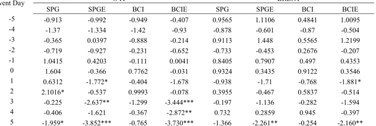
In this section, we present the results for both WTI and Brent crude oil, for each index, for the three types of OPEC’s decisions, as well as for the three sub-periods. Tables 2 and Figure 2 show CARs and their paths respectively for an increase in quotas announcements. According to other existing studies (Guidi et al., 2006; Bina and Vo, 2007; Lin and Tamvakis, 2010, Demirer and Kutan, 2010; Schmidbauer and Rösch, 2011; Mensi et al., 2014),whatever the commodity index and the oil price chosen, the results aregenerally not statistically significant.These results can be explained by OPEC’s so-called “cheating” behavior—showing norespect for the

18_{This effect has been observed in several commodity prices’ volatility levels (see Bowden and Payne, 2008). When}_γ_{is negative, the effect is called the}

(26)

25 quotas allocated to OPEC’s members—with the tendency to increase their production above the agreed quotas (Kaufmann et al., 2004; Lin and Tamvakis, 2010; Colgan, 2011). For example, Colgan (2011) has reported a 10% excess in production over OPEC members’ quota from1982 to 2009. OPEC may thus anticipate “cheating” by its members and adapt quotas accordingly. More generally, OPEC may endorse unilateral decisions made previously by its members.Another argument is put forward by Hyndman (2008). He explains the low significance of results by the fact that it is easier for OPEC’s members to agree on a quota increase, a behavior that can be readily anticipated by the market.Market participants donot react to an increase in production, as they seem to expect such decisions. However, the significance improves for the energy counterpart of the indices, as oil is a major constituent (except for WTI during the first sub-period, relative to BCI). For the vast majority, there is a significant impact on CARs after the announcement day. The market does not anticipate, and thus does not incorporate the information of an increase in production; but rather adjusts during the post-announcement period.

Table 2.1: CARs around OPEC Increase quotas (whole period)

Note: */**/*** indicates the t-statistic is significant at 10%/5%/1% level respectively. The following acronyms are used. WTI: West Texas Intermediate, SPG: Standard and Poors Commodity Index, BCI: Bloomberg Commodity Index, SPGE and BCIE are their energy counterparts.

Event Day WTI BRENT

SPG SPGE BCI BCIE SPG SPGE BCI BCIE

-5 -0.913 -0.992 -0.949 -0.407 0.9565 1.1106 0.4841 1.0095 -4 -1.37 -1.334 -1.42 -0.93 -0.878 -0.601 -0.87 -0.504 -3 -0.365 0.0397 -0.888 -0.214 0.9113 1.448 0.5565 1.2199 -2 -0.719 -0.927 -0.231 -0.652 -0.733 -0.453 0.2676 -0.207 -1 1.0415 0.4203 -0.111 0.0041 0.8405 0.7907 0.497 0.4353 0 1.604 -0.366 0.7762 -0.031 0.9324 0.3435 0.9122 0.3546 1 0.6312 -1.772* -0.404 -1.678 -0.938 -1.71 -0.768 -1.881* 2 2.1016* -0.537 0.9993 -0.078 0.3955 -0.467 0.5837 -0.514 3 -0.225 -2.637** -1.299 -3.444*** -0.197 -1.136 -0.282 -1.594 4 -0.406 -1.621 -0.367 -2.872** 0.732 0.2859 0.945 -0.397 5 -1.959* -3.852*** -0.765 -3.730*** -1.366 -2.261** -0.254 -2.160**

(27)

26

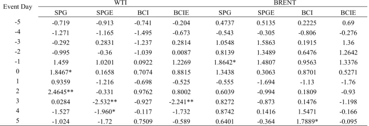
Table 2.2: CARs around OPEC Increase quotas (1991 Q1–2004 Q3)

Event Day WTI BRENT

-5 -0.719 -0.913 -0.741 -0.204 0.4737 0.5135 0.2225 0.69 -4 -1.271 -1.165 -1.495 -0.673 -0.543 -0.305 -0.806 -0.276 -3 -0.292 0.2831 -1.237 0.2814 1.0548 1.5863 0.1915 1.36 -2 -0.995 -0.36 -1.039 0.0087 0.8139 1.3489 0.6476 1.2642 -1 1.459 1.0201 0.0922 1.2269 1.8642* 1.4807 0.9563 1.3376 0 1.8467* 0.1658 0.7074 0.8815 1.3438 0.3063 0.8701 0.5271 1 0.9359 -1.216 -0.698 -0.525 -0.555 -1.694 -1.13 -1.76 2 _2.4645** _-0.331 _0.9762 _0.8002 _0.6039 _-0.994 _0.1809 _-0.93 3 0.0284 -2.532** -0.927 -2.241** 0.8272 -0.873 0.1476 -1.198 4 -1.527 -1.960* -0.117 -1.732 0.8742 0.1416 1.5471 -0.166 5 -1.024 -1.72 0.7509 -0.589 0.6401 -0.364 1.7889* -0.095

Table 2.3: CARs around OPEC Increase quotas (2005 Q1–2015 Q1)

Event Day WTI BRENT

-5 0.0794 -0.095 0.3036 -0.05 -0.13 -0.169 0.056 -0.091 -4 0.1802 -0.18 0.2615 -0.338 -0.4 -0.481 -0.207 -0.472 -3 0.7919 -0.063 0.8787 -0.603 -0.012 -0.271 0.3144 -0.375 -2 0.5619 -0.374 0.8725 -0.6 -0.553 -0.78 -0.104 -0.729 -1 0.4515 -0.804 0.4323 -1.239 -0.948 -1.217 -0.655 -1.34 0 0.4625 -0.69 0.5297 -1.008 -1.447 -1.647 -1.03 -1.628 1 0.1341 -1.425 0.2585 -1.616 -1.24 -1.495 -0.837 -1.564 2 -0.146 -1.31 -0.316 -1.366 -1.328 -1.425 -1.05 -1.382 3 _-0.926 _-2.097 _-2.197 _-2.913* _-2.044 _-2.049 _-2.397* _-2.542* 4 -0.183 -1.703 -2.349 -3.532** -2.947* -3.070* -3.565** -3.906** 5 0.1275 -1.498 -1.341 -3.145* -4.373** -4.464** -4.422** -4.881** Note: */**/*** indicates the t-statistic is significant at 10%/5%/1% level respectively. The following acronyms are used. WTI: West Texas

Intermediate, SPG: Standard and Poors Commodity Index, BCI: Bloomberg Commodity Index, SPGE and BCIE are their energy counterparts.

As expected, the CARs are negative in most cases. Indeed, an increase in oil production will drive prices down. Nevertheless, Figure 2 reveals that CARs may be positive, although more often insignificant.This result is more pronounced during the first sub-period and for Brent oil prices. A possible explanation could be as follows.On the one hand, OPEC often acts as a marginal producer (see, for example, Kaufmann, 2004) in order to offset, at least partially, the difference between oil demand and non-OPEC supply, using its spare production

(28)

27

capacity19.Between 1991 and 2004, we observe two phenomena. First, the consumption of crude oil constantly

increased, as did the production by both OPEC and non-OPEC producers. Second, the level of OPEC’s spare capacity dramatically plummeted between 1981 (around 14 million barrels (mb) per day) and 1990 (less than 2mbper day), whereas it fluctuated during the first sub-period between about 2 mb per day and 8 mb per day. On the other hand, non-OPEC oil producers are generally considered as price takers, meaning that they do not adjust their production to influence oil prices. Consequently, non-OPEC producers operate at or near full capacity and so have little spare capacity. Taking all these considerations together, it can be argued that an increase in OPEC’s production may be interpreted by market participants as a sign of tensions in the oil market, signaling a greater intervention of OPEC and thus resulting in higher future oil prices. The greater is the OPEC intervention, the greater is its impact on oil prices. However, OPEC’s diminishing spare capacity limits its ability to manipulate oil prices.

Fig.2.CAR paths for increase quota announcements for all periods.

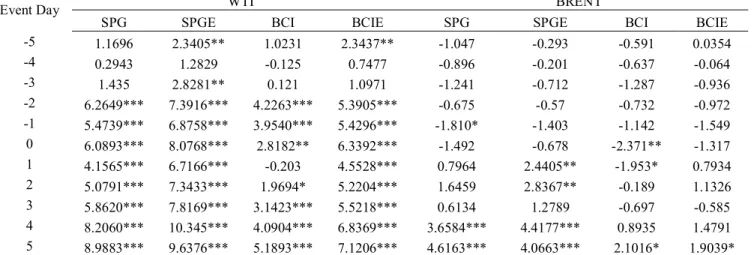
When a reduction in oil production is announced, the results, consistently with other papers mentioned above, are more significant than in the previous case (see Tables 3 and Figure 3).In general, WTI prices react more than Brent prices to OPEC’s cut announcements, whatever the index. Moreover, except for the second sub-period, the results seem more sensitive to S&P GSCI than to BCI. This can be explained by the weights of the WTI crude oil and Brent crude oil in these indices. Indeed, the weight of WTI crude oil is higher than that of Brent crude oil in

19_{The US Energy Information Administration (EIA) defines spare production capacity as the additional volume of production that can be brought on}

(29)

28 the two indices, even if, in recent years (notably since 2011), the proportion of WTI decreases in favor of Brent, though the latter has not overtaken the former yet. For example, the weight of WTI (Brent) in theS&P GSCI in 2011 and 2013 was 32.6% (15.9%) and 24.7% (22.1%), respectively. For BCI, the corresponding figures were 14.7% (0%) in 2011 and 9.2% (5.8%) in 2013. Moreover, the cumulated weights of WTI crude oil and of Brent crude oil in the S&P GSCI are much more important than those in the BCI. Similar to an increase in production quotas decisions, in most cases, the cut decisions have a significant effect after the announcement day. However, for the whole period and especially for the first sub-period, WTI returns responded significantly to those decisions before the announcement day (up to three days). It follows that when WTI prices fluctuate in a relatively narrow band, the market anticipates OPEC’s cut decisions. The significance is more pronounced for the first sub-period when prices are lower.

Table 3.1: CARs around OPEC Cut quota (whole period)

Event Day WTI BRENT

-5 _1.0654 _2.1977** _0.5377 _1.6423 _-0.672 _-0.178 _-0.646 _-0.066 -4 -0.077 1.1491 -1.084 0.1004 -1.108 -0.475 -1.357 -0.537 -3 1.0526 2.5101** -1.421 0.4258 -0.992 -0.577 -1.832* -0.8 -2 4.9594*** 6.1881*** 1.6233 3.6938*** -0.552 -0.309 -1.436 -0.726 -1 4.3605*** 5.5061*** 1.4622 3.6321*** -2.093* -1.689 -2.393** -1.761* 0 5.1300*** 6.7901*** 1.1624 4.7161*** -1.639 -0.816 -2.704** -1.346 1 3.3274*** 6.8082*** -1.636 3.7246*** -0.668 1.3256 -3.149*** 0.008 2 5.0297*** 7.7418*** 0.7496 4.7708*** 0.8996 2.3142** -0.909 1.0924 3 5.2433*** 6.9346*** 1.7764* 4.5189*** -0.352 0.5913 -1.442 -0.614 4 _8.9417*** _11.097*** _3.4826*** _6.8278*** _2.5129** _3.7759*** _0.3182 _1.6938 5 10.401*** 11.149*** 4.6224*** 7.8437*** 3.3224*** 3.5812*** 1.2033 2.3220** Note: */**/*** indicates the t-statistic is significant at 10%/5%/1% level respectively. The following acronyms are used. WTI: West Texas

(30)

29

Table 3.2: CARs around OPEC Cut quota (1991 Q1–2004 Q3)

Event Day WTI BRENT

-5 1.1696 2.3405** 1.0231 2.3437** -1.047 -0.293 -0.591 0.0354 -4 0.2943 1.2829 -0.125 0.7477 -0.896 -0.201 -0.637 -0.064 -3 1.435 2.8281** 0.121 1.0971 -1.241 -0.712 -1.287 -0.936 -2 6.2649*** 7.3916*** 4.2263*** 5.3905*** -0.675 -0.57 -0.732 -0.972 -1 5.4739*** 6.8758*** 3.9540*** 5.4296*** -1.810* -1.403 -1.142 -1.549 0 6.0893*** 8.0768*** 2.8182** 6.3392*** -1.492 -0.678 -2.371** -1.317 1 4.1565*** 6.7166*** -0.203 4.5528*** 0.7964 2.4405** -1.953* 0.7934 2 _5.0791*** _7.3433*** _1.9694* _5.2204*** _1.6459 _2.8367** _-0.189 _1.1326 3 5.8620*** 7.8169*** 3.1423*** 5.5218*** 0.6134 1.2789 -0.697 -0.585 4 8.2060*** 10.345*** 4.0904*** 6.8369*** 3.6584*** 4.4177*** 0.8935 1.4791 5 8.9883*** 9.6376*** 5.1893*** 7.1206*** 4.6163*** 4.0663*** 2.1016* 1.9039* Note: */**/*** indicates the t-statistic is significant at 10%/5%/1% level respectively. The following acronyms are used. WTI: West Texas

Table 3.3: CARs around OPEC Increase quota (2005 Q1–2015 Q1)

Event Day WTI BRENT

-5 -0.024 0.1417 -0.451 -0.735 -0.023 0.0694 -0.289 -0.266 -4 _-1 _-1.028 _-1.017 _-1.48 _-0.59 _-0.387 _-0.674 _-0.568 -3 -0.805 -1.96 -2.091 -2.087 0.0126 0.073 -0.651 -0.316 -2 -1.947 -3.050* -2.525* -3.120* -0.164 0.0123 -0.801 -0.601 -1 -2.249 -4.089** -2.34 -3.917** -1.611 -1.469 -1.985 -1.889 0 -2.627* -4.562** -2.718* -4.405** -1.292 -1.139 -1.76 -1.677 1 -1.475 -3.214** -2.109 -3.452** -2.317 -2.065 -2.711* -2.409* 2 -0.743 -2.361* -1.91 -2.961* -1.336 -1.104 -1.85 -1.547 3 -1.067 -3.086* -1.267 -3.170* -1.636 -1.498 -1.701 -1.67 4 1.9862 -0.075 0.1041 -1.395 -0.414 -0.254 -0.854 -0.622 5 _2.3457 _0.4086 _-0.086 _-1.193 _-1.17 _-0.909 _-1.761 _-1.221

Following a cut in production, oil prices should increase and consequently CARs should be positive. This is indeed the case for the whole period and the first sub-period for both WTIand Brent crude oils. However, during the second sub-period, significant CARs are negative and high for the two crude oil prices (see also Guidi et al., 2006; Lin and Tamvakis, 2010). Despite the OPEC cut announcement, oil prices have continued to decrease. OPEC’s cut decisions occurred in 2006, when oil prices fell significantly, and before the sharp increases in 2007 and 2008 (when prices peaked in July 2008). This apparently counterintuitive result may reflect considerations of market participants with regard to world current and future supply and demand for oil and their skepticism concerning the