HAL Id: hal-01312317
https://hal.archives-ouvertes.fr/hal-01312317
Submitted on 5 May 2016
HAL is a multi-disciplinary open access
archive for the deposit and dissemination of
sci-entific research documents, whether they are
pub-lished or not. The documents may come from
teaching and research institutions in France or
abroad, or from public or private research centers.
L’archive ouverte pluridisciplinaire HAL, est
destinée au dépôt et à la diffusion de documents
scientifiques de niveau recherche, publiés ou non,
émanant des établissements d’enseignement et de
recherche français ou étrangers, des laboratoires
publics ou privés.
Conservative dissipation: How important is the Jacobi
identity in the dynamics?
Cameron Caligan, Cristel Chandre
To cite this version:
Cameron Caligan, Cristel Chandre. Conservative dissipation: How important is the Jacobi identity
in the dynamics?. Chaos: An Interdisciplinary Journal of Nonlinear Science, American Institute of
Physics, 2016, 26, pp.053101. �10.1063/1.4948411�. �hal-01312317�
dynamics?
C.E. Caligan1,a)and C. Chandre2,b)
1)School of Physics, Georgia Institute of Technology, Atlanta, Georgia 30332-0430,
USA
2)Centre de Physique Th´eorique, CNRS / Aix-Marseille Universit´e, Campus de Luminy, 13009 Marseille,
France
(Dated: 5 May 2016)
Hamiltonian dynamics are characterized by a function, called the Hamiltonian, and a Poisson bracket. The Hamiltonian is a conserved quantity due to the anti-symmetry of the Poisson bracket. The Poisson bracket satisfies the Jacobi identity which is usually more intricate and more complex to comprehend than the conservation of the Hamiltonian. Here we investigate the importance of the Jacobi identity in the dynamics by considering three different types of conservative flows in R3: Hamiltonian, almost-Poisson and metriplectic.
The comparison of their dynamics reveals the importance of the Jacobi identity in structuring the resulting phase space.
Keywords: Hamiltonian systems, Casimir invariants, Jacobi identity, metriplectic systems
Hamiltonian systems are ubiquitous in many branches of physics, e.g., in atomic and molec-ular physics, in celestial mechanics, and in fluid and plasma physics, to name a few. These sys-tems display a finite or infinite number of de-grees of freedom depending on the complexity and modeling of the problem at hand. Hamil-tonian systems have the important property of being conservative, in the sense that there exists a conserved quantity, which is most often the en-ergy, called the Hamiltonian, and denoted by H in what follows. However Hamiltonian systems are much more than conservative systems. Hamilto-nian dynamics is generated by a Poisson bracket {·, ·}. The time-evolution of a given observable F (function of the dynamical variables) is given by
dF
dt = {F, H}.
This Poisson bracket is antisymmetric, bilinear and satisfies the Leibniz rule and the Jacobi iden-tity. The antisymmetry property, i.e., {F1, F2} =
−{F2, F1}, implies that the Hamiltonian is a
con-served quantity, i.e., dH/dt = 0. The richness of Hamiltonian systems resides in the Jacobi iden-tity :
{F1, {F2, F3}} + {F2, {F3, F1}} + {F3, {F1, F2}} = 0,
for all observables F1, F2 and F3. In general, this
identity makes it extremely difficult to deal with Hamiltonian systems, especially for non-canonical Hamiltonian systems1. For instance, performing
approximations on the equations of motion, e.g.,
a)Electronic mail: [email protected] b)Electronic mail: [email protected]
neglecting terms, usually breaks up this property if not done carefully. The natural question is how important is this property on the actual dynam-ics. Can we disregard this identity without affect-ing qualitatively the dynamics? Is it sufficient for a good model to be energy conserving in absence of dissipative terms?
Numerous conservative models in fluid and plasma physics are built without considering the Jacobi identity. In the field of nonlinear control theory, some works in the literature got rid of this property, and coined the result-ing systems, almost-Poisson (or pseudo-Poisson). These almost-Poisson systems are conservative systems (and the corresponding bracket satisfies the Leibnitz rule). However, due to the fact that the Jacobi identity is not satisfied, there is some dissipation associated with the almost-Poisson systems, which has been coined “fake dis-sipation” in Ref.2. This fake dissipation enters in
compe-tition with the dissipative terms introduced in the equa-tions of motion. For instance, models in fluid and plasma dynamics typically exhibit some dissipation modeling the interaction of the considered degrees of freedom with the ones which have been left out to derive a reduced (and hence more tractable) model. For instance, the effect of neglected degrees of freedom, e.g., associated with small scales, can be modeled by diffusion terms in the equa-tions of motion. In all these models, the ideal part which is obtained by removing the dissipative terms (e.g., the ones characterized by phenomenological constants, like diffusion coefficients, viscosity, collisionality...) should be Hamiltonian, reflecting the Hamiltonian character of the parent models (or from first principles) from which the reduced models have been constructed (e.g., Vlasov-Maxwell equations in plasma physics). Is it good enough to have an almost-Poisson model with some added dissi-pation? Or even in the dissipative case, is it still impor-tant to have the Jacobi identity for the ideal part of the model?
2
simple example for the importance of the Jacobi identity in the dynamics, which drastically affect the qualitative dynamics.
Here we consider flows in R3 given by the bracket
{F, G} = α · ∇F × ∇G,
where α = α(x, y, z) is a function from R3 to R3. This
bracket is bilinear and antisymmetric. Moreover it satis-fies the Leibniz rule for any function α. It satissatis-fies the Jacobi identity if and only if
α· ∇ × α = 0. (1) We notice that Nambu systems3 correspond to the case
where α = ∇S. In this case, the velocity ˙x = ∇H × α is divergence-free. This is not the case for all α sat-isfying Eq. (1). We recall that Casimir invariants are defined as observables which Poisson-commute with all the other observables. In particular it commutes with the Hamiltonian, and is therefore a conserved quantity. In our case, a Casimir invariant S(x, y, z) has to satisfy α × ∇S = 0. Therefore there exists a function λ(x, y, z) such that α = λ∇S from which it can be deduced that α· ∇ × α = 0. As a consequence, if the system possesses a Casimir invariant, the Jacobi identity is automatically satisfied. Moreover, if has been proved in Ref.4that there
exists two scalar functions λ and S such that the solution of Eq. (1) can be written locally as α = λ∇S. Thus S is a Casimir invariant. The Jacobi identity is locally equiv-alent to the existence of a Casimir invariant for flows in R3. If the system is almost-Poisson, there is no additional conserved quantity in general.
In order to illustrate its impact on the dynamics we consider Hamiltonian H and α given by
H(x, y, z) = cos(x + y + z), (2) α= (cos x, cos y, sin z + ε cos y). (3) We notice that for ε = 0 the system is Hamiltonian with a Casimir invariant
S(x, y, z) = sin x + sin y − cos z,
whereas for ε 6= 0, it is almost-Poisson since α · ∇ × α = −ε cos x sin y.
We consider a large ensemble of initial conditions on the plane x + y + z = π/4 and we integrate these trajec-tories for a rather long time (up to T = 1000) to observe the effect of dissipation. We monitor the conservation of the energy H and the Casimir invariant S. The equations of motion are
˙x = − sin(x + y + z)(sin z − cos y)
− ε cos y sin(x + y + z), (4a) ˙y = − sin(x + y + z)(− sin z + cos x)
+ ε cos y sin(x + y + z), (4b) ˙z = − sin(x + y + z)(cos y − cos x). (4c)
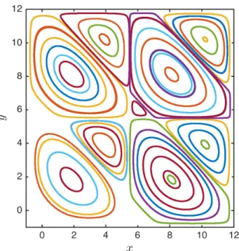
FIG. 1. Trajectories associated with Eqs. (4a-4c) with ǫ = 0. This corresponds to a Hamiltonian case.
The phase portrait is depicted in Fig. 1. As expected, we notice that energy and the Casimir invariant, depicted in Fig. 2, are conserved up to numerical precision. Al-most all trajectories are periodic given the fact that there are two conserved quantities. It is worth noting that the shape of the phase portrait, and in particular the ab-sence of attractors, is often attributed to the fact that the flow is divergence-free (or volume-preserving), which is the case here. However by choosing another function α= λ∇S, the phase portrait is exactly the same (even if the trajectories on these one-dimensional curves are dif-ferent) since these one-dimensional curves are defined by the two same conserved quantities H and S.
We compare the Hamiltonian dynamics ǫ = 0 with another conservative system obtained from Eqs. (4a-4c) with a slight modification, ǫ = 10−2. Typical
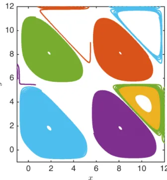
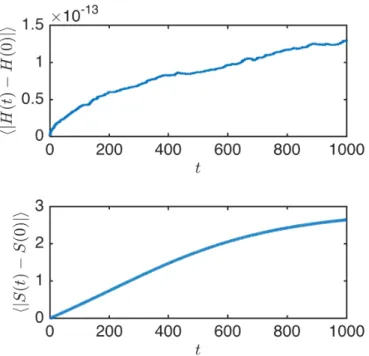
trajecto-ries are plotted in Fig. 3, and the associated variation of energy and Casimir invariant are plotted in Fig. 4. First we notice that the energy is conserved up to numerical precision. In addition, we clearly notice the presence of attractors even though this system is conser-vative. As expected, S is no longer a conserved quan-tity. For individual trajectories, S(t) is not monotonous, even if, on average, it appears to be monotonous. How-ever here the convergence towards attractors is very slow, which explains why the trajectories appear to fill densely some parts of phase space. We compared the dissipa-tive dynamics (ε 6= 0) to another type of dissipation, a metriplectic system2,5,6. The idea is to construct a
FIG. 2. Mean value of the energy variations (upper panel) and Casimir variations (lower panel) for System (4a-4c) with ǫ= 0. This corresponds to a Hamiltonian case.
from the following bracket
(F, G) = α · ∇F × ∇G + µ(∇F × ∇H) · (∇H × ∇G),
where µ = µ(x, y, z) is a positive function which will be chosen later. The bracket (·, ·) is bilinear but obviously not a Poisson bracket since it is not antisymmetric. In fact the part that has been added to the antisymmetric bracket {·, ·} is symmetric. We assume that {·, ·} is a Poisson bracket, and hence it has a Casimir invariant, denoted by S(x, y, z). We define the free energy as F0=
H − S. We define the dynamics as
dF
dt = (F, F0).
We notice that H is a conserved quantity by construction (S being a Casimir invariant of the Poisson part of the bracket). Moreover, the dynamics of S verifies
dS
dt = µk∇S × ∇Hk
2≥ 0,
which means that the entropy grows with time mono-tonically. In the numerical example, we consider µ = ¯
µ/ sin2(x + y + z) where ¯µ is a constant. The equations
FIG. 3. Trajectories of System (4a-4c) with ǫ = 10−2. This
corresponds to an almost-Poisson case.
of motion for the metriplectic systems become: ˙x = − sin(x + y + z)(sin z − cos y)
+ ¯µ(−2 cos x + cos y + sin z), (5a) ˙y = − sin(x + y + z)(− sin z + cos x)
+ ¯µ(cos x − 2 cos y + sin z), (5b) ˙z = − sin(x + y + z)(cos y − cos x)
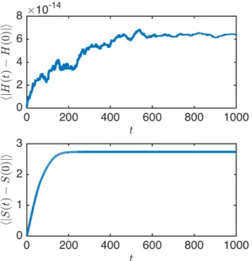
+ ¯µ(cos x + cos y − 2 sin z). (5c) The system is conservative in the sense that H = cos(x + y+z) is a conserved quantity. It is dissipative in the sense that it is not Hamiltonian for ¯µ 6= 0. The phase portrait is depicted in Fig. 5 and the values of the variations of H and S are represented on Fig. 6. We emphasize that the integration time for System (5a-5c) is the same as the one for System (4a-4c). However both types of dis-sipation result in significantly different phase portraits. The dissipation introduced in the metriplectic system is much stronger leading to a fast convergence towards at-tracting fixed points. This is also seen in Fig. 6 where the convergence of the mean value of the variations of S is much stronger in the metriplectic system than in the almost-Poisson case.
The comparison of the numerics shows that, even though the energy is conserved to a high accuracy, the dynamics exhibited by the two dissipative systems, built from the same ideal part, are very different. This rein-forces the importance of the type dissipative terms intro-duced in the equations.
In summary, we have shown on a simple example, Hamiltonian flows in R3, that the Jacobi identity shapes
4
FIG. 4. Mean value of the variations of H (upper panel) and S (lower panel) for System (4a-4c) with ǫ = 10−2. This
corresponds to an almost-Poisson case.
the dynamics by preventing the existence of attractors. For instance, we have emphasized the strong links be-tween the Jacobi identity and the existence of Casimir in-variants. These invariants foliate phase space, preventing unphysical transport across phase space. Despite the fact that systems are energy-conserving, Hamiltonian systems exhibit a qualitatively different dynamics that almost-Poisson systems or metriplectic systems. Of course, these results are particular to Hamiltonian flows in R3, but the
link between Casimir invariants has also been noticed for infinite dimensional Hamiltonian systems, for instance, for fluid reductions of the Vlasov equation, and for Dirac brackets of constrained Hamiltonian systems7,8.
ACKNOWLEDGMENTS
The research leading to these results has received fund-ing from the People Program (Marie Curie Actions) of
the European Union’s Seventh Framework Program No. FP7/2007-2013/ under REA Grant No. 294974. CC ac-knowledges useful discussions with P.J. Morrison.
1P.J. Morrison, Rev. Mod. Phys. 70, 467 (1998) 2P.J. Morrison, Physica 18D, 410 (1986) 3Y. Nambu, Phys. Rev. D 7, 2405 (1973)
4A. Ay, M. Gurses, and K. Zheltukhin, J. Math. Phys. 44, 5688 (2003)
5D. Fish, Metriplectic systems (PhD thesis, Portland State Uni-versity, 2005)
6A.M. Bloch, P.J. Morrison, and T.S. Ratiu, in Recent Trends in
FIG. 5. Trajectories of System (5a-5c) with ¯µ= 10−2. This
corresponds to a metriplectic case.
Dynamical Systems, eds. A. Johann et al., Springer Proceedings in Mathematics and Statistics 35, 371 (2013)
7M. Perin, C. Chandre, P.J. Morrison, E. Tassi, J. Phys. A: Math. Theor. 48, 275501 (2015)
FIG. 6. Mean value of the variations of H (upper panel) and S (lower panel) for System (5a-5c) with ¯µ= 10−2. This