Symbolic controller synthesis for timed systems: robustness and optimality

(1)

HAL Id: tel-02436831

https://hal.archives-ouvertes.fr/tel-02436831

Submitted on 13 Jan 2020

HAL is a multi-disciplinary open access

archive for the deposit and dissemination of sci-entific research documents, whether they are

pub-L’archive ouverte pluridisciplinaire HAL, est destinée au dépôt et à la diffusion de documents scientifiques de niveau recherche, publiés ou non,

Symbolic controller synthesis for timed systems:

robustness and optimality

Damien Busatto-Gaston

To cite this version:

Damien Busatto-Gaston. Symbolic controller synthesis for timed systems: robustness and optimality. Computer Science and Game Theory [cs.GT]. Aix Marseille Université, 2019. English. �tel-02436831�

(2)

AIX-MARSEILLE UNIVERSITÉ

ED 184 MATHEMATIQUES ET INFORMATIQUE

LABORATOIRE D’INFORMATIQUE ET SYSTEMES

Thèse présentée pour obtenir le grade universitaire de docteur

Discipline: Informatique

Damien Busatto-Gaston

Synthèse symbolique de contrôleurs pour systèmes temporisés:

robustesse et optimalité

Symbolic controller synthesis for timed systems: robustness and optimality

Soutenue le 03/12/2019 devant le jury composé de:

Nathalie Bertrand (CR)INRIA Rennes Bretagne-Atlantique Examinatrice

Patricia Bouyer-Decitre (DR)CNRS, LSV, ENS Paris-Saclay Examinatrice

Krishnendu Chatterjee (PR)IST Austria Rapporteur

Benjamin Monmege (MCF)LIS, CNRS, Aix Marseille Université Directeur

Joël Ouaknine (PR)MPI for Software Systems Rapporteur

Laure Petrucci (PR)LIPN, CNRS, Université Paris 13 Examinatrice

Pierre-Alain Reynier (PR)LIS, CNRS, Aix Marseille Université Directeur

(3)

Remerciements

J’aimerais tout d’abord remercier Benjamin et Pierre-Alain pour le soutien constant et les conseils précis qu’ils m’ont fournis au cours de cette thèse. Ces trois années enrichissantes furent un plaisir par leur encadrement et leur bienveillance.

Je voudrais également remercier Krishnendu Chatterjee, Joël Ouaknine et Igor Walu-kiewicz pour avoir été rapporteurs de ce document, ainsi que Nathalie Bertrand, Laure Petrucci et Patricia Bouyer-Decitre pour s’être intéressées à mes travaux en tant que membres du jury. Je remercie en particulier cette dernière pour m’avoir fait découvir ce sujet, m’avoir conseillé et m’avoir orienté vers Marseille lorsque j’étais en master.

Si le nom, les locaux et la direction du LIS ont changé au cours de ces dernières années, il est resté un laboratoire particulièrement chaleureux et agréable, dont j’aimerais remercier les membres permanents pour leur acceuil, et les non-permanents pour leur complicité et leur entrain. Merci à mes co-bureaux Florian, Didier, Eloi d’avoir supporté ma tendance récurrente à faire les cents pas. Je remercie particulièrement Sébastien R. pour m’avoir assuré sans failles, ainsi que Théodore, Amélia, Manon P., Léo E., José Luis, Thibault, Manon S., Cindy, Franck, Pacôme, Jeremy, Cedric, Sébastien D. et les autres pour nos échanges scientifiques ou ludiques réguliers. Je remercie aussi mes amis, et en particulier Léo T. et Antoine pour leur coopération.

Je remercie enfin ma famille pour leurs encouragements constants, leurs efforts pour s’intérésser à mes travaux et leur bonne humeur.

(4)

Résumé

Le domaine de la synthèse réactive a pour objectif d’obtenir un système correct par construction à partir d’une spécification logique. Une approche classique consiste à se ramener à un jeu à somme nulle, où deux joueurs interagissent tour-à-tour dans un système de transitions, et à se demander si le joueur "contrôleur" peut garantir que son objectif sera rempli, et ce indépendamment des décisions du joueur "environnement". Nous étudions des spécifications temps-réel, modélisées par un automate temporisé équipé d’un objectif d’accessibilité ou de Büchi, et présentons des méthodes symboliques pour synthétiser des stratégies du contrôleur. Nos contributions concernent deux problématiques distinctes : on peut souhaiter que le contrôleur obtienne une stratégie robuste aux perturbations, ou bien le faire jouer de manière optimale dans un jeu pondéré. Dans le contexte de la robustesse, le contrôleur a pour objectif de suivre un lasso acceptant de l’automate. De plus, ses choix de délais successifs doivent résister à d’éventuelles perturbations choisies par l’environnement. Ce problème est connu comme étant PSPACE-complet, mais les techniques existantes opèrent sur l’abstraction des régions. Nous proposons une solution moins sensible à une explosion de l’espace d’états, en faisant exclusivement usage de zones. Dans le contexte quantitatif, nous étudions des jeux sur automates temporisés équipés de poids : le contrôleur souhaite minimiser le poids accumulé en atteignant un état cible, alors que l’environnement vise l’objectif opposé. Dans une perspective de synthèse réactive, cette extension pondérée des jeux temporisés permet de mesurer le degré de qualité du contrôleur. Les jeux temporisés pondérés sont rapidement indécidables, même lorsque les poids sont tous positifs. Des résultats de décidabilité existent pour une classe à poids positifs, définie par une restriction sémantique sur le poids des cycles. Nous introduisons la classe des jeux temporisés pondérés divergents comme une généralisation de cette restriction sémantique autorisant les poids négatifs, ce qui permet de représenter par exemple de l’énergie ou de l’argent. Nous présentons une méthode pour calculer la valeur optimale de ces jeux. Les jeux divergents forment donc la première classe décidable de jeux temporisés pondérés avec des poids négatifs et un nombre arbitraire d’horloges. Nous étudions enfin une classe plus générale introduite par Bouyer, Jaziri et Markey en 2015, qui reste analysable lorsque les poids sont positifs. Bien que cette classe soit indécidable, les auteurs montrent que l’on peut approximer la valeur du jeu en utilisant des régions de granularité moindre. Nous étendons cette classe pour autoriser des poids négatifs, et montrons que la valeur y reste approximable. De plus, nous expliquons qu’un algorithme symbolique suivant le paradigme de value iteration peut être utilisé sur cette classe en tant que schéma d’approximation.

(5)

Abstract

The field of reactive synthesis studies ways to obtain, starting from a specification, a system that is correct by construction. A classical approach models this setting as a zero-sum game played by two players on a transition system, and asks whether player controller can ensure an objective against any competing player environment. We focus on real-time specifications, modelled as timed automata with reachability or Büchi acceptance conditions, and present symbolic ways to synthesise strategies for the controller. We consider two problems, either restricting controller to robust strategies or aiming for optimal strategies in a weighted game setting. In the robustness setting, the goal of the controller is to play according to an accepting lasso of the automaton, while resisting to timing perturbations chosen by a competing environment. The problem was previously shown to be PSPACE-complete using regions-based techniques, but we provide a first tool solving the problem using zones only, thus more resilient to state-space explosion issues. In the quantitative setting, we study games played on a timed automaton equipped with weights: controller wants to minimise the accumulated weight while reaching a target, while the environment has an opposite objective. In a reactive synthesis perspective, this quantitative extension of timed games allows one to measure the quality of controllers. Weighted timed games are notoriously difficult and quickly undecidable, even when restricted to non-negative weights. Decidability results exist for a subclass with non-negative weights defined by a semantical restriction on the weights of cycles. We introduce the class of divergent weighted timed games as a generalisation of this semantical restriction to arbitrary weights, allowing one to model energy for instance. We show how to compute their optimal value, yielding the first decidable class of weighted timed games with negative weights and an arbitrary number of clocks. Then, we focus on a larger class, known to be analysable with non-negative weights, that has been introduced by Bouyer, Jaziri and Markey in 2015. Though the value problem is undecidable, the authors show how to approximate the value by considering regions with a refined granularity. We extend this class to incorporate negative weights, and prove that the value can still be approximated. In addition, we show that a symbolic algorithm, relying on the paradigm of value iteration, can be used as an approximation schema on this class.

(6)

11.Approximating values 151 11.1. Kernel of an almost-divergent WTG. . . 152 11.2. Semi-unfolding of almost-divergent WTGs . . . 154 11.2.1. Semi-unfolding construction . . . 155 11.2.2. Semi-unfolding correctness . . . 156 11.3. Approximation of almost-divergent WTGs . . . 159 11.3.1. Approximation of kernels . . . 159

(9)

11.3.2. Approximation of almost-divergent WTGs . . . 162

11.4. Example of an execution of the approximation schema . . . 163

11.5. Symbolic approximation algorithm . . . 167

11.5.1. Discussion . . . 170

(10)

Introduction

The widespread use of digital technology can be felt in most aspects of modern life. Digital systems are designed to assist with—and sometimes perform autonomously—important tasks, from long-distance communications to the management of our electrical or financial infrastructures. When faced with a known situation, we trust these systems to act accordingly, with near-instantaneous reaction times. This holds particularly for embedded systems, i.e. systems designed to perform a fixed task, as part of a broader structure. They can be found in most electronic devices, from phones and home appliances to traffic lights, avionics and elevators. This has prompted a large research effort in computer science, where a series of work has been devoted to the creation, analysis and testing of embedded systems, as they are sometimes entrusted with our safety.

This is a challenging task, as the correctness or reliability of a system can depend on fine interactions with its surroundings or with other systems, and it can be hard, for the human designer, to anticipate on all possible behaviours.

Computer-aided verification

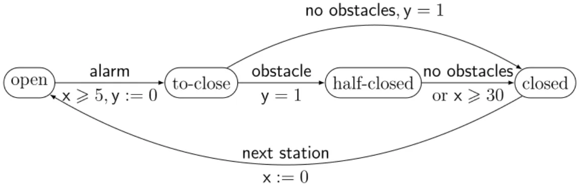
One approach lies in the field of formal methods, where one studies a mathematical idealisation of the system, called a model, to check that it satisfies some desired properties, such as eventually performing a particular task, or avoiding errors. The objective is to develop automated methods to analyse and verify systems. For example, the model-checking problem asks if a given model satisfies its specification, described by a logical formulæ. This problem has been extensively studied in various settings, with practical tools being used for the verification of hardware and software in industry (see e.g. [CHVB18]). half-closed closed to-close open obstacle no obstacles obstacle alarm wait no obstacles next station

(11)

Example 1. As an example, we will use an embedded system that controls a pair of

doors in a subway train, represented in Figure 1. Whenever the train arrives at a new

station, the doors open. The system waits until an alarm signals departure for the next station, then checks for any obstacles to their closing. If such an obstacle is present, the doors close partially, and wait until the obstacle is removed before closing. Desired property for the system might be "the train must always travel with closed doors", or "doors always eventually close". The former is always guaranteed by this model, but not the latter, that requires additional assumptions (we do not wait forever for the departure signal, and obstacles are always eventually removed).

An ambitious variant is that of controller synthesis, where one starts from the specifica-tion alone. The goal is to build a model that will, by construcspecifica-tion, be correct. A classical approach expresses this problem from the viewpoint of game theory: One encodes all possible behaviours in a transition system, where two players are opposed. Starting from some initial state for the system, the player named controller makes decisions that determine how the system dynamically evolves. Thus, a sequence of successive states is obtained, and we want this sequence to satisfy the specification. Examples include asking that a target "good" state is eventually reached, or conversely that an error "bad" state is never reached. However, the controller may sometimes not get to choose the next state, in which case we say that the decision is made by the second player, called the environment. The notion of environment captures everything that cannot be anticipated, from user inputs to complex interactions with the real world or foreign systems. Overall, the way the system evolves is derived from the choices of both players in a turn-based fashion, and this interaction forms a game, where controller wins if its objective is met. Our goal is thus to automatically construct a strategy for the controller, that is a recipe dictating how to play, so that controller wins no matter how the environment plays. Such strategy finally describes a system that is necessarily correct, since the specification must hold in all possible scenarios.

Example 2. Going back to the example of Figure 1, one could consider that whether an

obstacle is present or not is not under our control. As such, player controller can choose whether to wait, ring the alarm, or go to the next station when in the appropriate states, but player environment is the one that decides if there is an obstacle or not.

Timed systems

We focus on a class of programs sensitive to real-time, where keeping track of how much time elapses between the decisions taken by the program is required to differentiate the good and bad behaviours. This is a common requirement for embedded systems, as they interact with the real world. The design of such programs is a notoriously difficult problem, because they must take care of delicate timing issues, and are difficult to debug a posteriori. In order to ease the design of real-time software, it appears important to automatise the process by using formal methods. The situation may be

(12)

half-closed closed to-close open no obstacles or x > 30 obstacle y = 1 alarm x > 5, y := 0 no obstacles, y = 1 next station x := 0

Figure 2.: A timed automaton modelling train doors.

real-valued variables, called clocks, evolving with a uniform rate. Transitions are equipped with timing constraints expressed over the clocks, and may only be taken when these constraints are met.

Example 3. We enrich the train door example from Figure 1, in order to obtain the

timed automaton depicted on Figure 2. Clocks x, y are variables that continuously

increase, at a rate of one unit per second. Whenever the train arrives at a new station, clock x is reset (i.e. set to 0). We must stay in the open state at least five seconds before signalling departure, at which point clock y is reset. Exactly one second later, the system closes the doors if possible, and otherwise goes to the half-closed state. We then wait until either the obstacle is removed or the time since arrival at the current station (recorded by x) is at least thirty seconds, in which case we forcefully close the doors and

leave.1 Note that we removed the waiting loops in the open and half-closed states, as

they are no longer needed: in a timed automaton, one can always stay in the current state and let time elapse.

In order to verify the real-time system, one determines whether there exists an accepting execution in the timed automaton. A simple, yet realistic specification asks that a target state is reached at some point. We are also interested in Büchi acceptance conditions, where a target should be reached infinitely often along the execution, modelling cases where we do not want the system to get stuck in a bad situation. It has been proven

in [AD94] that the reachability and Büchi problems on timed automata are both

PSPACE-complete, by partitioning the state space into regions. While optimal from a theoretical complexity point of view, practical tools tend to favour efficient symbolic algorithms for solving these problems, that use zones instead of regions, as they allow an on-demand partitioning of the state space. This leads to much better performances, as

witnessed by successful model-checking tools like Uppaal [LPY97], Kronos [BDM+₉₈_],

or TChecker [HPT19, HSW10].

In this thesis, we study two controller synthesis problems on timed automata, either restricting controller to robust strategies or aiming for optimal strategies in a weighted game setting. The document is split into three parts:

(13)

half-closed closed to-close alarm x < 30 closing x > 30 y = 1

Figure 3.: A timed automaton with Zeno behaviours.

• In PartI, we recall formalisms and known techniques for the study of finite or timed transition systems;

• In Part II, we focus on making choices that are robust with regard to small timing

perturbations;

• In PartIII, we present results on weighted timed games, where one aims for optimal

choices in a quantitative setting.

Robustness

As we have seen, timed automata [AD94] provide an automata-theoretic framework to

design, model and verify real-time systems. However, the semantics of timed automata is a mathematical idealisation: it assumes that clocks have infinite precision and that actions are instantaneous. Proving that a timed automaton satisfies a property may not ensure that a real implementation of it also does. This robustness issue is a challenging

problem for embedded systems [HS06], and alternative semantics have been proposed, so

as to ensure that the verified (or synthesised) behaviour remains correct in presence of small timing perturbations.

Example 4. As an example, consider Figure3, that models part of a variant of Figure2:

We assume that there is an obstacle that is not removed, and we add an action that lets us repeat the alarm signal until the thirty seconds mark has been reached. We argue that some infinite behaviours of this system are not realistic, as it is possible to ring the alarm infinitely many times with a so-called Zeno behaviour. Indeed, one could let one second elapse, and use the alarm transition once. Then, we let half a second elapse, and

use it again. By using increasingly smaller delays (1/2i after i steps), the alarm can be

rung arbitrarily many times, while keeping the total time elapsed under two seconds. Another issue lies in the steps that require infinite precision, like the transition from the to-close to the half-closed state. Indeed, it requires clock y to be valued at exactly

1. This might prove hard to ensure with a real system, and it would be preferable in

this case to leave some margin η > 0 around 1, such that one asks for y ∈ [1 − η, 1 + η] instead.

We are interested in a fundamental model-checking problem in timed automata equipped with a Büchi condition: it consists in determining whether there exists an

(14)

accepting infinite execution. This problem has been studied numerously in the exact

set-ting, where symbolic methods have been developed [TYB05,Tri09,Li09,HS10,HSW12,

LOD+13, HSTW16]. In the context of robustness, the execution should be tolerant to

small perturbations of the delays. This discards executions suffering from weaknesses such as Zeno behaviours, or even non-Zeno behaviours requiring infinite precision, as exhibited in [CHR02].

More formally, the semantics we consider is defined in Chapter 3 as a game that

depends on some parameter δ representing an upper bound on the amplitude of the perturbation [CHP11]. In this game, the controller plays against an antagonistic environ-ment that can perturb each delay using a value chosen in the interval [−δ, δ]. The case

of a fixed value of δ has been shown to be decidable in [CHP11], and also for a related

model in [LLTW14]. However, these algorithms are based on regions, and as the value of

δ may be much smaller than the constants appearing in the guards of the automaton, do

not yield practical algorithms. Moreover, the maximal perturbation is not necessarily known in advance, and could be considered as part of the design process.

The problem we are interested in is qualitative: we want to determine whether there exists a positive value of δ such that the controller wins the game. It has been proven in [SBMR13] that this problem is in PSPACE (and even PSPACE-complete), thus no harder than in the exact setting with no perturbation allowed. However, the algorithm,

recalled in Chapter 4, heavily relies on regions, and more precisely on an abstraction

that refines the one of regions, namely folded orbit graphs. Hence, it is not amenable to implementation, and has indeed never been implemented. Our main contribution

in Part II is to provide, in Chapter 5, an efficient symbolic algorithm for solving this

problem.

Our algorithm can be understood as an adaptation to the robustness setting of the

standard algorithm for Büchi acceptance in timed automata [LOD+₁₃_{]. This algorithm}

looks for an accepting lasso using a nested breadth-first search. A major difficulty consists in checking whether a lasso can be robustly iterated, i.e. whether there exists δ > 0 such that the controller can follow the cycle for an infinite amount of steps while being tolerant to perturbations of amplitude at most δ.

Our approach relies on several new ingredients:

• We provide a polynomial time procedure to decide, given a lasso, whether it can be robustly iterated. This symbolic algorithm relies on a computation of the greatest fixpoint of the operator describing the set of controllable predecessors of a path. In order to provide an argument of termination for this computation, we resort to a new notion of branching constraint graphs, extending the approach used in [JR11,Tra16]

and based on constraint graphs (introduced in [CLJ99]) to check iterability of a

cycle, without robustness requirements.

• We provide a termination criterion for the analysis of lassos. Focusing on zones is not complete: it can be the case that two cycles lead to the same zone, but one is robustly iterable while the other one is not. Robust iterability crucially depends on the real-time dynamics of the cycle and we prove that it actually only depends on

(15)

the reachability relation of the path. We provide a polynomial-time algorithm for checking inclusion between reachability relations of paths in timed automata based on constraint graphs.

• It is worth noticing that all our procedures can be implemented using difference bound matrices, a very efficient data structure used for timed systems. These developments have been integrated in a tool, and we present a case study of a train regulation network illustrating its performances.

We finally study in Chapter 6 a quantitative variant, where one computes the greatest

value of δ such that the controller wins the game. We obtain a new decidability result for this problem, by showing that when considering a lasso, not only can we decide robust iterability, but we can even compute the largest perturbation under which it is controllable.

Weighted timed games

Solving the robustness game for a fixed value of δ can be seen as an instance of a more general problem, where both players alternatively choose transitions and delays. This is a natural extension of the controller synthesis problem to the real-time setting called a timed game, where a controller and an antagonistic environment play on a timed automaton instead of a finite transition system. Strategies of players become recipes dictating how to play on this arena (timing delays and transitions to follow). In this more ambitious setting, we will focus on reachability objectives, and we are thus looking for a strategy of the controller so that the target is reached no matter how the environment

plays. Reachability timed games are decidable [AM99], and EXPTIME-complete [JT07].

If the controller has a winning strategy in a given reachability timed game, several such winning strategies could exist. Weighted extensions of these games have been considered

in order to measure the quality of the winning strategy for the controller [BCFL04].

This means that the game, defined in Chapter 8, now takes place over a weighted (or

priced) timed automaton [BFH+01, ALTP04], where edges are equipped with weights,

and locations with rates of weights (the cost is then proportional to the time spent in this location, with the rate as proportional coefficient).

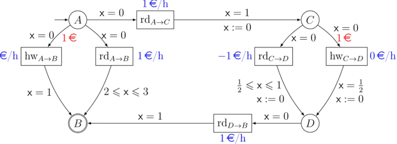
Example 5. As a motivating example for studying weighted games, we present a

ride-sharing scenario. As a driver, we wish to travel from point A to point B, and must

choose between several options, as displayed in Figure 4. We can use a direct road, and

reach B in two to three hours, or an highway that lets us reach our destination in one hour. Alternatively, we can make a detour: another traveller is waiting at point C, and wishes to reach point D. For this portion too, a faster highway is available.

While all four possible paths satisfy the objective "reaching B", we want to select the one that lets us spend as little money as possible for the trip. The cost of each path depends on several factors. There are fixed entry fees (of 1 e) for the highways, and we need to keep track of fuel consumption, as the rate at which fuel is used differs in roads

(16)

A C B D road 1h road 1h road [2h, 3h] highway 1h highway 0.5h road [0.5h, 1h]

Figure 4.: A ride-sharing decision diagram.

A rdA→B hwA→B rdA→C B C rdC→D hwC→D D rdD→B 1e/h 1e/h

2e/h 1e/h −1e/h 0e/h

x = 0 x = 1 x := 0 x = 0 ₁_e x = 1 x = 0 2 6 x 6 3 x = 0 1 2 6 x 6 1 x := 0 x = 0 1e x = 1₂ x := 0 x = 0 x = 1

Figure 5.: A weighted timed game modelling Figure 4. The cost of waiting in a state

is displayed in blue, the cost of taking a transition is in red. States and transitions without costs have a weight of 0 e

and highways. Thus, we say that roads cost 1 e per hour, while highways cost 2 e per hour. Moreover, if we share the portion from C to D, the other traveller will pay for his trip (at a rate of 2 e/h), and that can lower our costs. A shared road therefore costs us −1 e per hour (negative rate means we are making a profit), while a shared highway costs 0 e/h.

The situation can be modelled as a weighted timed game, displayed in Figure 5. The

controller chooses delays and transitions in circle states, while the environment controls the square ones. For example, if we choose to use the direct road from A to B, we go (immediately) to state rdA→B, and stay there until going to state B. This requires letting

between two and three hours elapse in rdA→B, with a cost of 1 e/h. The delay is chosen

by the environment, as it depends on external influences like traffic density.

In this example, the optimal strategy is to share the road from C to D. This lets us ensure a total weight of at most 1.5 e: going from A to C costs 1 e in the worst case; going from D to B similarly costs at most 1 e; and sharing the trip from C to D is guaranteed to bring us at least 0.5 e.

(17)

While solving weighted timed automata has been shown to be PSPACE-complete [BBBR07] (i.e. the same complexity as the non-weighted version), weighted timed games are known

to be undecidable [BBR05]. This has led to many restrictions in order to regain

decid-ability, the first and most interesting one being the class of strictly non-Zeno cost with

only non-negative weights (in edges and locations) [BCFL04]: this hypothesis states that

every execution of the timed automaton that follows a cycle of the region abstraction has a weight far from 0 (in interval [1, +∞), for instance).

Less is known for weighted timed games in the presence of negative weights in edges and locations. In particular, no results exist so far for a class that does not restrict the number of clocks of the timed automaton to 1. However, negative weights are particularly interesting from a modelling perspective, for instance in case weights represent the consumption level of a resource (money, energy. . . ) with the possibility to spend and

gain some resource. In Chapter9, we introduce a generalisation of the strictly non-Zeno

cost hypothesis in the presence of negative weights, that we call divergence. We show the decidability of the class of divergent weighted timed games for the optimal synthesis

problem in Chapter 10:

• We describe a procedure to solve weighted timed games for a bounded horizon, i.e. when controller has a fixed number of steps to reach his targets. It follows

closely the framework of [ABM04], but is more symbolic and allows for negative

weights.

• We show that optimal strategies in divergent weighted timed games can be restricted to a bounded horizon, that matches the one obtained in the non-negative case from

the study of [BCFL04].

The techniques providing these decidability results cannot be extended if the conditions are slightly relaxed. For instance, if we add the possibility for an execution of the timed automaton following a cycle of the region automaton to have weight exactly 0, the decision

problem is known to be undecidable [BJM15], even with non-negative weights only. For

this extension, in the presence of non-negative weights only, it has been proposed an approximation schema to compute arbitrarily close estimates of the optimal weight that

the controller can guarantee [BJM15]. To this end, the authors consider regions with a

refined granularity so as to control the precision of the approximation.

Our contribution on the approximation front is presented in Chapter11, and is two-fold:

• We extend the class considered in [BJM15] to the presence of negative weights, and

provide an approximation schema for the resulting class of almost-divergent games; • We show that the approximation can be obtained using a symbolic computation,

that avoids an a priori refinement of regions.

Moreover, the classes of weighted timed games that we study induce interesting classes of finite weighted game when there are no clocks, that can be solved with a lower

(18)

Part I.

(19)

1. Finite systems

Let us now formally introduce transition systems and their quantitative or game-theoretical extensions. In this chapter we study finite systems only, but terminology and notations are defined over infinite ones with further chapters in mind.

1.1. Transition systems

Definition 1.1. Let Σ be a set of elements called labels. A transition system labelled

over Σ is a pair hS, T i, with S a set of states and T ⊆ S × Σ × S a set of transitions, such that (s, a, s0_{) ∈ T} _{is denoted s}₋_{→ s}a 0_.

A transition system is finite if it has finitely many states and transitions. A directed graph labelled over Σ is a finite transition system hS, T i (labelled over Σ), such that T contains at most one transition from s to s0 _{for every pair of state (s, s}0₎_{. A relation R}

over a domain Q is a set of pairs in Q × Q, and we sometimes write a R b to denote that the pair (a, b) belongs to R. A relation is complete if it equals Q × Q. A graph hS, T i induces a relation over the finite domain S as {(s, s0_{) | ∃a ∈ Σ, s}₋_{→ s}a 0_}_{: the set of states}

(s, s0) linked by a transition. It is complete if this relation is complete.

For k > 1, a finite path of length k is a finite sequence of transitions (si, ai, s0i)16i6ksuch

that for all i ∈ [1, k−1], s0

i = si+1. Such a path ρ will be denoted s1 a1 −→ s2 a2 −→ . . . sk ak −→ s0 k,

and is said to be a path from state first(ρ) = s1 to state last(ρ) = s0k of length |ρ| = k.

The concatenation of two finite paths ρ1 and ρ2, such that last(ρ1) = first(ρ2), is denoted

by ρ1ρ2. Transitions can be seen as paths of length one and states as paths of length

zero, and we extend the first and last operators in those cases. A cycle is a finite path ρ, of length at least 1, such that first(ρ) = last(ρ).

We similarly define an infinite path ρ ∈ TN as an infinite sequence of transitions

s0 a1

−→ s1 a2

−→ . . ., with first(ρ) = s0. A state s is called a deadlock state if there are no

transitions t ∈ T with first(t) = s. A path ρ is maximal if it is infinite or if it is finite and ends in a deadlock state. Conversely, a non-maximal path is a finite path that can be extended.

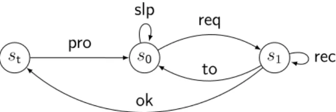
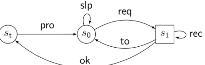
Example 1.1. Figure1.1represents a transition system labelled over {req, rec, ok, pro, slp, to}, that models a client interacting with a server. From an initial state s0, the client sends a

request for data by taking the transition labelled by req. The server should answer by sending a finite sequence of data, activating the receive transition rec multiple times. The communication should end with a confirmation as the ok transition, allowing the client to process the data with pro and return to the initial state. The client can sleep in the initial state with slp, and if the communication fails the client will time-out with transition to.

(20)

s0 s1 st req to slp rec ok pro

Figure 1.1.: A transition system modelling a client that requests a sequence of data to a server, receives it and processes it.

In this analogy, the finite path s0 req −→ s1 rec −→ s1 ok −→ st pro −→ s0 req −→ s1 to −→ s0 represents an

execution of the client where a successful interaction is followed by a time-out. There are no deadlock states in this transition system, and therefore every maximal path is infinite and every finite-path is non-maximal.

A finite (resp. infinite) path s0 a1

−→ s1 a2

−→ . . . naturally induces a finite (resp. infinite)

word a0a1. . . over labels. A set of infinite words L is called an ω-language. Given a

transition system and an initial state s0, the ω-language Ls0 is defined as the set of

infinite words over labels induced by the infinite paths that start from s0. If the transition

system is finite, it can be seen as a non-deterministic Büchi automata where every state is accepting, and therefore its language is an ω-regular language, a notion that generalises the notion of regular languages to infinite words.

Definition 1.2. Given a transition system hS, T i, an objective Lt (as an ω-language

over labels) and an initial state s0, the emptiness problem asks if Ls0∩ Lt 6= ∅, i.e. is

there an infinite path starting from s0 that induces a word in Lt.

Definition 1.3. Given a transition system hS, T i, an objective Lt (as an ω-language

over labels) and an initial state s0, the model-checking problem asks if Ls0 ⊆ Lt, i.e. does

every infinite path starting from s0 induce a word in Lt.

The objective language encodes a specification, and can be expressed as an ω-regular expression or a formula in linear temporal logic (LTL) for example. We will be focusing on simple objectives, like the reachability of a target or a Büchi condition.

Definition 1.4. Given a transition system hS, T i, an initial state s0 ∈ S and a set of

target states St⊆ S, the emptiness problem with a reachability condition asks if there

exists a finite path ρ such that first(ρ) = s0 and last(ρ) ∈ St. The emptiness problem

with a Büchi condition asks if there exists an infinite path s0 a1

−→ s1 a2

−→ . . . starting from s0 that reaches St infinitely often, i.e. such that there exists infinitely many i ∈ N with

si ∈ St.

One can observe that the emptiness problem with a reachability (resp. Büchi) condition is a particular case of the emptiness problem, as we could extend if needed the label of every transition t with the states first(t) and last(t) and thus express these conditions on words over labels. We call the associated ω-language a reachability (resp. Büchi) objective.

(21)

Example 1.2. Consider the transition system in Figure 1.1, the initial state s0 and

the target states St = {st}. The emptiness problem with reachability condition St

is satisfied, as st is reachable from s0 by following req and ok. Since st can return

to s0 with pro, the emptiness problem with Büchi condition St is also satisfied. The

corresponding reachability (resp. Büchi) objective is the ω-language of all infinite words over {req, rec, ok, pro, to} that contain at least one (resp. infinitely many) ok. The model-checking problem is not satisfied with these objectives, as it is possible to loop between s0 and s1 infinitely many times for example, never reaching st.

These problems have been well studied in a variety of settings, and we now give a few results that apply to finite systems only. The emptiness problem with a reachability condition can be solved in linear time using forward exploration techniques, like the classical breadth-first search algorithm. Such techniques can indeed compute the set

of states reachable from s0, which is enough for reachability conditions. For Büchi

conditions, one can then launch a second exploration from every reachable state st in St

and search for a loop around st. A linear time complexity can be obtained by computing

all strongly connected components. Model checking is polynomial for reachability and

Büchi objectives, as it can be solved by attractor computations (see Section1.3.1).

1.2. Weighted transition systems

All of the problems defined so far have been qualitative in nature. In order to model quantitative notions like the cost of going from a source to a destination, we need to define concepts such as the weight of a path, or the weight of a set of paths. This can be done by considering a setting where labels are real numbers, the weight of a path is the sum of its labels and the weight of a set of paths is the minimum of the weight of each path. This is the setting that we will consider in our study of timed systems, and our problems can be seen as extensions of the classical shortest path problem. However, some developments (Difference Bound Matrices with non-standard entries) will require the same notions over more exotic labels, so we introduce the more general context of

[BT10], where labels are only required to form a set with some algebraic properties.

1.2.1. Semirings, closure operation

A binary operation ⊕ over a domain Q is a mapping from Q × Q to Q, and we sometimes write a ⊕ b to denote the element ⊕(a, b).

Definition 1.5. A semiring (Q, ⊕, ⊗, 0, 1) is a set Q equipped with two binary operations

⊕and ⊗ over Q of respective neutral element 0 and 1, such that for all a, b, c ∈ Q:

• (⊕ is associative) (a ⊕ b) ⊕ c = a ⊕ (b ⊕ c) • (0 is neutral for ⊕) 0 ⊕ a = a ⊕ 0 = a • (⊕ is commutative) a ⊕ b = b ⊕ a

(22)

• (⊗ is associative) (a ⊗ b) ⊗ c = a ⊗ (b ⊗ c) • (1 is neutral for ⊗) 1 ⊗ a = a ⊗ 1 = a

• (⊗ distributes over ⊕, left) a ⊗ (b ⊕ c) = (a ⊗ b) ⊕ (a ⊗ c) • (⊗ distributes over ⊕, right) (a ⊕ b) ⊗ c = (a ⊗ c) ⊕ (b ⊗ c) • (0 is absorbing for ⊗) 0 ⊗ a = a ⊗ 0 = 0

Examples of semirings include the natural semiring (N, +, ×, 0, 1), equipped with stand-ard addition and multiplication over integers, the tropical semiring (N∪{+∞}, min, +, +∞, 0), or the boolean semiring ({0, 1}, ∨, ∧, 0, 1). As the neutral elements 0 and 1 are uniquely

determined by ⊕ and ⊗ 1_{, we may omit them and refer to the semiring as (Q, ⊕, ⊗), or}

simply Q if the operations are clear from context. If 0 = 1 then necessarily Q = {0}, and Q is called the trivial semiring. The classical notion of ring additionally requires that every element of Q has an inverse by ⊕ in Q, i.e. ∀a ∈ Q, ∃(−a) ∈ Q such that

a ⊕ (−a) = 0. Semirings strictly generalise rings, as for examples the boolean semiring

({0, 1}, ∨, ∧)is not a ring.

Definition 1.6. A relation v ∈ Q × Q is a (partial) order if for all a, b, c ∈ Q

• (v is reflexive) a v a

• (v is transitive) a v b ∧ b v c ⇒ a v c • (v is antisymmetric) a v b ∧ b v a ⇒ a = b

An ordered semiring is a semiring (Q, ⊕, ⊗) such that the relation v defined as

{(a, b) | ∃c ∈ Q, a ⊕ c = b} is an order on Q. The relation v is always reflexive and

transitive by the properties of ⊕, but it is not antisymetric on every semiring. In fact, a non-trivial ring cannot be an ordered semiring. For example, (R>0, +, ×) is an ordered

semiring with v equal to the standard 6 order on R>0, but (R, +, ×) is not ordered by v.

If (Q, ⊕, ⊗) is a semiring where ⊕ is selective (i.e. ∀a, b ∈ Q, a ⊕ b = a ∨ a ⊕ b = b), then

(Q, ⊕, ⊗) is an ordered semiring, and v is a total order (i.e. ∀a, b ∈ Q, a v b ∨ b v a).

Thus, another example of ordered semirings is (R ∪ {+∞}, min, +), with v equal to the > order over reals. If (Q, ⊕, ⊗) is an ordered semiring, then for every subset Q0 ⊆ Qsuch that ⊕ and ⊗ are stable over Q0 _{and such that 0 and 1 are in Q}0_{, (Q}0_{, ⊕, ⊗)} _{is also an}

ordered semiring. Therefore, (N, +, ×) and (Q ∪ {+∞}, min, +) are ordered semirings. If (Q, ⊕, ⊗) is an ordered semiring, then 0 is the least element of Q w.r.t. v, i.e. ∀a ∈

Q, 0 v a. If there exists in Q an absorbing element ∞ for ⊕ (such that for all a ∈ Q,

∞ ⊕ a = ∞), then ∞ is the greatest element of Q w.r.t. v, i.e. ∀a ∈ Q, a v ∞.

For example, (R>0∪ {+∞}, min, +) and ({0, 1}, ∨, ∧) are ordered semirings where ∞

equals 0 and 1, respectively. If Q does not contain an absorbing element for ⊕, we can consider a new symbol ∞ 6∈ Q and extend ⊕ and ⊗ with a ⊕ ∞ = ∞ for a ∈ Q,

(23)

∞ ⊕ ∞ = ∞, a ⊗ ∞ = ∞ ⊗ a = ∞ for a ∈ Q\{0}, 0 ⊗ ∞ = ∞ ⊗ 0 = 0 and

∞ ⊗ ∞ = ∞, such that (Q ∪ {∞}, ⊕, ⊗, 0, 1) is an ordered semiring with ∞ absorbing

for ⊕. This allows us to define the ordered semirings (R>0∪ {+∞}, +, ×)with ∞ = +∞

and (R ∪ {+∞, −∞}, min, +) with ∞ = −∞ for example, and in the following we will assume that every ordered semiring contains an absorbing element ∞ for ⊕.

For every k > 0 and a ∈ Q in an ordered semiring (Q, ⊕, ⊗), let ak denote 1 if

k = 0 and N_06i<ka (i.e. a ⊗ a · · · ⊗ a, k times) if k > 0, and let a(k) denote L_06i6kai (i.e. a0_{⊕ · · · ⊕ a}k). On ordered semirings, ⊕ is monotone (i.e. ∀a, b ∈ Q, a v a ⊕ b), and

therefore the sequence (a(k)₎

k∈N is non-decreasing. Let a(∗) be called the closure of a and

denote the supremum of (a(k)₎

k∈N if it exists. Intuitively, a(∗) is the limit of the infinite

sum 1 ⊕ a ⊕ (a ⊗ a) ⊕ (a ⊗ a ⊗ a) ⊕ . . . in Q.

Definition 1.7. An ordered semiring with closure is an ordered semiring where the

closure a(∗) _{of every a ∈ Q exists, i.e. the set S}

a = {b ∈ Q | ∀k ∈ N, a(k) v b} contains

an element a(∗) such that a(∗) _{v b} for every b ∈ S a.

A first class of ordered semirings with closure are those where 1 = ∞, i.e. the neutral

element for ⊗ is absorbing for ⊕. In this case, a(∗) _{= 1} _{for every a ∈ Q. The semirings}

(R>0∪ {+∞}, min, +)and ({0, 1}, ∨, ∧) belong to this class. We now introduce another

class of ordered semirings with closure, called complete semirings.

The relation v is a complete order over Q if each of its subsets has a supremum, i.e. for all subsets S of Q, there exists c in B = {b ∈ Q | ∀a ∈ S, a v b} such that c v b for every

b ∈ B. In this case, we say that Q equipped with v is a complete join semilattice, where

join is the operator that returns the supremum of a subset of Q. A complete semiring is an ordered semiring (Q, ⊕, ⊗) such that the relation v is a complete order over Q.

Lemma 1.1. Complete semirings are ordered semirings with closure.

Proof. Consider some element a ∈ Q, and let fa be a unary operator over Q defined by

fa(q) = (a ⊗ q) ⊕ 1. In particular, fa(0) = 1 = a(0), and for every k > 0, fa(a(k)) = a(k+1).

Let us prove that fa is non-decreasing, by considering q1 v q2 (i.e. ∃c, q2 = q1⊕ c) and

showing fa(q1) v fa(q2):

fa(q2) = fa(q1⊕ c) = (a ⊗ (q1⊕ c)) ⊕ 1 = (a ⊗ q1) ⊕ (a ⊗ c) ⊕ 1 = fa(q1) ⊕ (a ⊗ c) .

It follows that on a complete semiring, fa is Scott-continuous (it preserves the supremum

of sets), and by Kleene’s fixpoint theorem [SHLG94], fa has a least fixpoint, which is the

supremum of the non-decreasing chain

0 v fa(0) v fa(fa(0)) v fa(fa(fa(0))) · · ·

i.e. the supremum of (a(k)₎

k∈N, and therefore a(∗) by definition.

Example 1.3. Some examples of complete semirings include (R_>0∪ {+∞}, +, ×), where

a(∗) equals +∞ if a > 1 and 1/(1 − a) if a < 1, and (R ∪ {−∞, +∞}, min, +) where

(24)

v where join is either the usual sup or inf operator over reals. (N ∪ {+∞}, +, ×) and (N ∪ {+∞}, min, +) are also complete semirings, but not (Q ∪ {−∞, +∞}, min, +) as the ordinary order > is not complete over rational numbers (the infimum of a subset of Q

may be irrational). However, if we let QN = {a/N | a ∈ Z} be the set of rational numbers

of granularity 1/N for a fixed N ∈ N>0, then the semiring (QN ∪ {−∞, +∞}, min, +)

is complete, and the closure operation is inherited from the tropical semiring over R ∪ {−∞, +∞}.

Let us denote Mn(Q) the set of n × n matrices over Q. If (Q, ⊕, ⊗) is an ordered

semiring, then, for every integer n > 0, (Mn(Q), ⊕, ⊗, 0, 1)is an ordered semiring, with

⊕ and ⊗ the entrywise addition and the standard multplication of matrices (using ⊕

and ⊗ over Q internally), 0 the null matrix (equal to 0 everywhere), and 1 the identity

matrix (equal to 1 on the diagonal and to 0 everywhere else). The order v over Mn(Q)

is inherited by applying the order v over Q entrywise, and for every matrix A ∈ Mn(Q),

A(∗) _{denotes the closure of A in the matrix semiring (i.e. 1 ⊕ A ⊕ A}2_{⊕ A}3_{⊕ . . .}_{) when it}

exists.

Lemma 1.2 (Generalized Gauss-Jordan, [GM08]). If (Q, ⊕, ⊗) is an ordered semiring

with closure, then A(∗) _{exists for every matrix A, so that (M}

n(Q), ⊕, ⊗) is also an

ordered semiring with closure. Moreover, A(∗) can be computed by performing at most n3

elementary operations (⊕, ⊗, and closure in Q).

This result is derived from a generalised version of the Floyd-Warshall algorithm

defined over semirings, described in Algorithm 1.1. To get intuition on Algorithm1.1,

one can interpret the matrix A as a graph G = h{1, . . . , n}, {i−−−→ j | M (i, j) 6= 0}iM (i,j)

labelled over Q, such that the entry (i, j) in A(∗) corresponds to applying L, over all

paths ρ from i to j in G, on N_ka

−

→l∈ρa. The closure of diagonal entries corresponds to

an acceleration of this computation over cycles, such that only paths without cycles need

to be considered. Whenever the variable k is incremented, Ak contains the result of this

computation over all paths without cycles that only use {1, . . . , k} as intermediate states,

and thus An⊕ 1 = A(∗) (that last step only updates diagonal entries by adding 1, this

corresponds to paths of length zero).

1.2.2. Transition systems labelled over a semiring

The results of this section hold for every semiring, but as we will mostly consider semirings that extend the tropical semiring in further chapters, we will change notations and name the two operators min and + of neutral elements +∞ and 0 instead of ⊕ and ⊗ of neutral elements 0 and 1. We will also assume that min has an absorbing element named −∞ instead of ∞. In this section, we consider only finite transition systems (finitely many states and edges).

Definition 1.8. A weighted transition system is a transition system hS, T i labelled over

(25)

Algorithm 1.1:Closure computation over the semiring of matrices [GM08]

Input : A ∈ Mn(Q)

Output : A(∗)

/* We construct a sequence of matrices A0. . . An */

1 A₀ ← A 2 for k ← 1 to n do 3 Ak(k, k) ← (Ak−1(k, k))(∗) 4 for i ← 1 to n do 5 for j ← 1 to n do 6 if (i, j) 6= (k, k) then

7 A_k(i, j) ← A_k−1(i, j) ⊕ (A_k−1(i, k) ⊗ A_k(k, k) ⊗ A_k−1(k, j))

8 return A_n⊕ 1

The weight of a finite path ρ = s0 a1

−→ s1. . . ak

−→ sk is obtained by summing its edges in

order (+ may not be commutative) wt(ρ) = a1+· · ·+ak. The weight wtk(s, s0)for a pair of

states (s, s0₎_{and k ∈ N is defined as the minimal weight of the set of all paths from s to s}0

of length exactly k in the transition system.2 We also let wt6k_{(s, s}0_{) = min}

06i6kwti(s, s0)

denote the minimal weight for all paths of length at most k ∈ N. From the ordering v of

(Σ, min, +)we derive an ordering 6, such that a 6 b ⇔ b v a ⇔ ∃c ∈ Σ, a = min(b, c).

The sequence (wt6k_{(s, s}0₎₎

k∈N is decreasing for 6, and we define wt(s, s0)as its infimum

w.r.t. 6 if it exists. In fact, we will see that it always exists when (Σ, min, +) is a semiring with closure.

Example 1.4. If the semiring is the tropical semiring (N ∪ {+∞}, min, +), then wt(s, s0)

corresponds to the weight of the shortest path from s to s0 _{in a transition system labelled}

by non-negative weights representing distance, and equals +∞ if no such path exists.

If the semiring is (Z ∪ {−∞, +∞}, min, +), wt(s, s0₎ _{corresponds to the infimum of the}

weight of the paths from s to s0_{, i.e. the weight of the shortest path if it exists, +∞ if s}

cannot reach s0_{, and −∞ if s can reach a negative cycle that can reach s}0_{. If the semiring}

is ({0, 1}, ∨, ∧), wt(s, s0_{) = 1}_{if and only if there is a path from s to s}0 _{entirely labelled}

by 1.

The adjacency matrix of a transition system hS, T i weighted over Σ is a matrix M in M|S|(Σ), seen as a mapping from S × S to Σ, such that M(s, s0) is equal to wt1(s, s0).

M is an element of the ordered semiring with closure (M|S|(Σ), min, +), where min

is the entrywise application of min and + is the standard product of matrices over (Q, min, +). Observe that for every pair of states (s, s0), it holds that for every k > 0, M(k)_{(s, s}0_{) = wt}6k_{(s, s}0₎_{, and therefore M}(∗)_{(s, s}0_{) = wt(s, s}0₎_{. Then, we can compute}

wt(s, s0)for every pair (s, s0) by using Algorithm1.1 on M. From the adjacency matrix

2_{In particular, wt}k_{(s, s}0_{) equals +∞ if there are no such path, and wt}0_{(s, s}0_{) is equal to 0 if s = s}0 _and

(26)

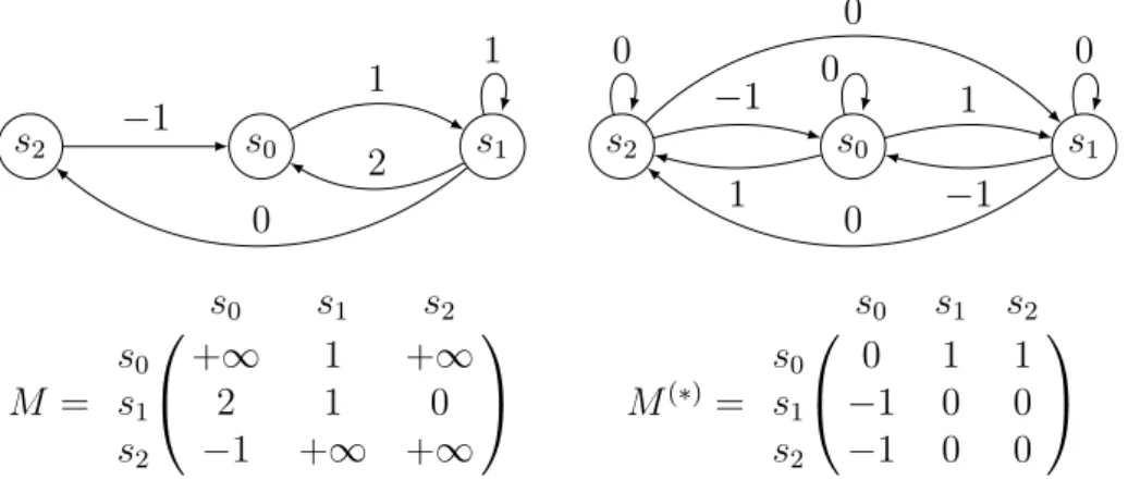
s0 s1 s2 1 2 1 0 −1 M =   s0 s1 s2 s0 +∞ 1 +∞ s1 2 1 0 s2 −1 +∞ +∞   s2 s0 s1 0 0 0 1 −1 1 −1 0 0 M(∗) =   s0 s1 s2 s0 0 1 1 s1 −1 0 0 s2 −1 0 0  

Figure 1.2.: A weighted transition system labelled over (Z ∪ {+∞, −∞}, min, +) and its adjacency matrix on the left, their closure on the right.

M(∗) of a transition system hS, T i, we can extract a transition system hS, T0_i_{called the}

closure of hS, T i, with T0 _{= {s}_{−−−−−→ s}M(∗)(s,s0) 0 _{| s, s}0 _{∈ S}}_.

Example 1.5. Figure 1.2 represents a transition system labelled over the tropical

semiring (Z ∪ {+∞, −∞}, min, +), its adjacency matrix M containing the minimum weight over paths of length 1, the closure M(∗) _{= min(1, M, M}2_{, M}3₎ _{(1 is the identity}

matrix with 0 on the diagonal and +∞ everywhere else), and the transition system associated with M(∗)_.

On (N ∪ {+∞}, min, +), Algorithm 1.1 is equivalent to running the classical

Floyd-Warshall algorithm on a graph with non-negative weights. On the semiring (Z ∪

{−∞, +∞}, min, +), Algorithm 1.1 is equivalent to running the Floyd-Warshall

al-gorithm on a graph with arbitrary weights, with an additional check that sets diagonal entries to −∞ as soon as they become negative.

1.3. Turn-based game on a transition system

In order to model situations where some choices are out of our control, we will study a game-theoretical extension of transition systems, where two players play a turn-based game.

Definition 1.9. A two-player turn-based game labelled over Σ is a tuple G = hSCtrl, SEnv, T i

such that SCtrl∩ SEnv = ∅and hSCtrl∪ SEnv, T i is a transition system labelled over Σ.

The disjoint union of states is denoted S = SCtrl] SEnv. We say that SCtrl contains the

states that belong to the player Ctrl, and SEnv the states that belong to the player Env. A

maximal play (resp. a non-maximal play) ρ in G is a maximal path (resp. a non-maximal

path) in hS, T i. Let S⊥⊆ S denote the deadlock states. Recall that states can be seen

as paths of length 0, and therefore states in S\S⊥ can be seen as non-maximal plays.

(27)

s0 s1 st req to slp rec ok pro

Figure 1.3.: A two-player turn-based game, where controller owns the circle states s0

and st, and the environment owns the rectangle state s1.

FPlaysP. A strategy σP for player P is a mapping from FPlaysP to T , such that for all

ρ ∈ FPlaysP, last(ρ) = first(σP(ρ)). A strategy is said positional if for all ρ ∈ FPlaysP,

σP(ρ) = σP(last(ρ)).3 Let play(s0, σCtrl, σEnv) denote the unique maximal play obtained

from an initial state and a pair of strategies, such that first(play(s0, σCtrl, σEnv)) = s0, and

for every prefix ρ of play(s0, σCtrl, σEnv)in FPlaysP, the next transition in play(s0, σCtrl, σEnv)

is σP(ρ).

Definition 1.10. Given a game G, an objective Lt (as an ω-language over labels) and

an initial state s0, the controller synthesis problem asks if there exists a strategy σCtrl for

Ctrl such that for all strategies σEnv for Env, play(s0, σCtrl, σEnv) is an infinite play that

induces a word in Lt.

Example 1.6. Figure 1.3 represents a two-player turn-based game associated with the

transition system of Figure1.1, such that SCtrl = {s0, st} and SEnv = {s1}. This models

the fact that, as a client, we do not control the server’s answer. On this example, consider the reachability objective associated with St= {st}, that models the specification "at

least one communication goes well". The synthesis problem is not satisfied from s0

with this objective, since for every strategy of player Ctrl, player Env can choose to always time-out, or loop in s1 forever. If we consider the specification "controller sends

at least one request", defined by the reachability objective associated with St = {s1},

the synthesis problem is satisfied from s0, for example with the positional strategy for

controller that chooses req in s0 and pro in st.

If SEnv is empty, the controller synthesis problem on G is equivalent to the emptiness

problem on the transition system hSCtrl, T i. If SCtrl is empty, the controller synthesis

problem on G is equivalent to the model-checking problem on the transition system hSEnv, T i.

For a finite system equipped with a reachability or Büchi objective, the controller synthesis problem is polynomial, and can be solved with fixpoint computations. In a more general setting where the objective is given as an LTL formula, the controller synthesis

problem is 2-EXPTIME complete [PR89].

3_{Positional strategies are often called memoryless in the literature, as they always make the same}

(28)

1.3.1. Attractors

We now recall the classical notion of attractor of a player towards a set of states, that is

used to solve reachability games. Let St ⊆ S be a set of states. The attractor of Ctrl

towards St is the set of states such that player Ctrl can guarantee reaching St eventually.

Formally, it is the greatest set S0 _{⊆ S} _{such that for all s ∈ S}0_{, either:}

1. s ∈ St; or

2. s ∈ SCtrl, and there exists a transition s a

−

→ s0 _{with s}0 _{∈ S}0_{; or}

3. s ∈ SEnv, and for all transitions s a

−

→ s0_{, it holds that s}0 _{∈ S}0_.

It is well-known that S0 _{can be computed with a fixpoint computation that starts with}

S0 = St, and adds progressively the states that satisfy conditions 2 or 3, until no such

state is left. The complexity of this computation is linear in the size |S| + |T | of the graph.4

Then, the controller synthesis problem with reachability objective St and initial state

s0 is satisfied if and only if s0 belongs to the attractor of Ctrl towards St, and in this

case one can extract from the attractor computation a (positional) strategy σCtrl that

guarantees reachability of St from s0.

A symmetrical notion of attractor of Env towards a set Stcan be defined and computed

similarly.

4_{A single backwards breadth-first search from S}

t is enough if one keeps track, for each state of Max, of

the number of successors that have not yet been added to S0. When this counter reaches 0 the state is added.

(29)

2. Timed systems

In this chapter, we introduce notions that let us express timing constraints, define timed automata as finite transition systems enriched by those notions, and introduce classical tools for their study.

2.1. Modelling real-time constraints

Let X = {x1, . . . , xn} be a finite, non-empty set of variables called clocks. A

valu-ation ν : X → R>0 is a mapping from clocks to non-negative real numbers, such that

ν(x1), . . . , ν(xn)are called the coordinates of ν. Equivalently, ν can be seen as a point in

space RX

>0. We denote 0 the valuation such that for all x ∈ X , ν(x) = 0. Given a real

number d ∈ R, we define ν + d as the valuation such that ∀x ∈ X , (ν + d)(x) = ν(x) + d

if it exists.1 _{If d is non-negative, we say that we performed a time elapse of delay d.}

The time-successors of ν are the valuations ν + d with d > 0. Similarly, we refer to all

ν + d in RX_>0 with d 6 0 as time-predecessors of ν. The set of points that are either

time-predecessors or time-successors of a valuation ν form the unique diagonal line in RX>0that contains ν. If Y is a subset of X , we define ν[Y := 0] as the valuation such that

∀x ∈ Y, (ν[Y := 0])(x) = 0 and ∀x ∈ X \Y, (ν[Y := 0])(x) = ν(x). This operation is called

a reset of clocks Y.

We extend those notions to sets of valuations in a natural way. The set of time-successors

of Z ⊆ RX

>0, denoted PostTime(Z), contains the valuations that are time-successors of

valuations in Z. The reset of Z ⊆ RX

>0 by Y, denoted Z[Y := 0], contains the valuations

ν[Y := 0] such that ν ∈ Z.

The term atomic constraint will refer to a linear inequality in one of the following forms:

• A strict (resp. non-strict) non-diagonal atomic constraint over clock x ∈ X and constant c ∈ Q is an inequality of the form x ./ c with ./ ∈ {>, <} (resp. ./ ∈ {>, 6}).

• A strict (resp. non-strict) diagonal atomic constraint over clocks x and y ∈ X and constant c ∈ Q is an inequality of the form x − y ./ c with ./ ∈ {>, <} (resp. ./ ∈ {>, 6}).

Let > and ⊥ denote two special atomic constraints, defined as x > 0 and x < 0 for an arbitrary x ∈ X . A guard g over X is a finite conjunction of atomic constraints over clocks in X . In particular, guards let us define x = c as shorthand for x 6 c ∧ x > c, and

1

(30)

c1 < x < c2 as shorthand for x > c1 ∧ x < c2 . A guard is said strict (resp. non-strict,

diagonal, non-diagonal) if all of its atomic constraints are strict (resp. non-strict, diagonal,

non-diagonal). Guards(X ) denotes the set of all guards over X , and Guardsnd

(X ) the subset of non-diagonal guards. For all constants c ∈ Q and ./ ∈ {>, 6, >, <}, we say

that valuation ν ∈ RX

>0 satisfies the atomic constraint x ./ c (resp. x − y ./ c), and write

ν |= x ./ c (resp. ν |= x − y ./ c), if ν(x) ./ c (resp. ν(x) − ν(y) ./ c). We say that

valuation ν ∈ RX

>0 satisfies guard g, and write ν |= g, if ν satisfies all atomic constraints

in g. For g ∈ Guards(X ), let JgK denote the set of all ν ∈ R

X

>0 such that ν |= g. Such

sets are called zones and form convex polyhedra of RX

>0. A guard g is said satisfiable

when the zone JgK is non-empty, and a zone is called rectangular when the associated

guard is non-diagonal. The universal zone refers toJ>K = R

X

>0 and the empty zone refers

to J⊥K = ∅. Guard g is the closed version of a satisfiable guard g where every strict

constraint of comparison operator < or > is replaced by its non-strict version 6 or >.

The zone JgK is the topological closure of Z = JgK, and is also denoted Z .

Zones are closed by intersection as JgK ∩ Jg

0

K = Jg ∧ g

0

K, but not by union.

2 Zones are

closed by time-successors as PostTime(JgK) is equal to Jg0

K, where g

0 _{is obtained from g}

by removing every non-diagonal atomic constraint of the form x < c or x 6 c. Zones are also closed by reset of clocks Y ⊆ X , asJgK [Y := 0] = Jg

0

K, where g

0 _{= ⊥} _if

JgK = ∅,

and otherwise g0 _{is obtained from g by removing every non-diagonal atomic constraint}

of the form x > c or x > c with x ∈ Y, replacing every diagonal atomic constraint of the form x − y ./ c with y ∈ Y (resp. x ∈ Y) by x ./ c (resp. y 6./ −c), and adding the constraint x 6 0 for every x ∈ Y. Note that encoding zones by storing their associated guard syntactically as a formula is not efficient, as guards can contain useless constraints. Moreover, it is possible to have different guards associated to the same zone, and for example testing if a zone is equal to another zone is non-trivial in this form.

2.2. Encoding constraints as DBMs

A bound (over R) is a pair (≺, c) with ≺ ∈ {<, 6} and c ∈ R. It represents the (open or large) upper bound ≺ c in a linear inequality. We introduce additional bounds (<, +∞)and (<, −∞) that will be used for trivial inequalities, and let Bounds(R) denote ({<, 6} × R) ∪ {(<, +∞), (<, −∞)}.

We say that a real number a ∈ R satisfies (≺, c) ∈ {<, 6} × R if the inequality a ≺ c holds. The bound (<, +∞) is satisfied by every real and (<, −∞) is never satisfied. We say that bound (≺, c) is at least as strong as (≺0_{, c}0₎_{, denoted (≺, c) 4 (≺}0_{, c}0₎_{, if all reals}

satisfying (≺, c) satisfy (≺0_{, c}0₎_{, equivalently if}

c = −∞ ∨ c0 = +∞ ∨ c < c0∨ (c = c0∧ (≺ = ≺0 ∨ ≺ = <)) .

This forms a total order over bounds, where the strongest bound is (<, −∞) and the weakest one is (<, +∞). We define a binary operator min over bounds that returns the strongest bound out of its arguments, and an infimum inf over sets of bounds that

(31)

returns the weakest bound that is at least as strong as every bound in the set. We also define an addition + such that

(≺, c) + (≺0, c0) = (≺00, c + c0) , with ≺00_{set to 6 if ≺ = ≺}0

= 6 and to < otherwise, and where c + c0 uses the + operator

of the tropical semiring (R ∪ {−∞, +∞}, min, +).3

The min operation admits (<, +∞) as neutral element and (<, −∞) as absorbing element, and + admits (6, 0) as neutral element and (<, +∞) as absorbing element. Then, (Bounds(R), min, +) is a semiring that we call the tropical semiring of bounds over R. It is an ordered semiring because min is selective. The order v induced by min in (Bounds(R), min, +) is {(a, b) | b 4 a}. Then, (Bounds(R), min, +) forms a complete join semilattice with v where join is the inf operator. Therefore, (Bounds(R), min, +) is an ordered semiring with closure. The closure of a bound (≺, c) is equal to: (<, 0) if (≺, c) = (<, 0); (<, −∞) if c < 0; and (6, 0) otherwise (i.e. if (6, 0) 4 (≺, c)).

We define bounds over a subset Q of R with Bounds(Q) = ({<, 6}×Q)∪{(<, +∞), (<, −∞)}

in a similar fashion. Recall that QN denotes the rational numbers of granularity 1/N

with N ∈ N>0, and consider the tropical semiring of bounds over QN, defined as

(Bounds(QN), min, +). It inherits the properties of (Bounds(R), min, +) and is an ordered

semiring with closure.

For notational convenience, we add a variable x0 that is always considered equal to

0, and denote X0 the set X ∪ {x0}. A difference bound constraint is a linear inequality

x − y ≺ c over clocks x, y ∈ X0 and bound (≺, c). As for atomic constraints, we say that a

valuation ν ∈ RX

>0satisfies x−y ≺ c and write ν |= x−y ≺ c if the real number ν(x)−ν(y)

satisfies the bound (≺, c) (with ν(x0) defined as equal to 0), and Jx − y ≺ cK denotes

the set of valuations that satisfy x − y ≺ c. The inclusion relation of sets of valuations in RX

>0 gives a natural order over atomic constraints, difference bound constraints and

guards. Thus, given atomic constraints, difference bound constraints or guards φ and φ0, we will say that φ is at least as strong as φ0 if _{JφK ⊆ Jφ}0_{K, and that φ is equivalent} to φ0 _if

JφK = Jφ

0

K. A difference bound constraint x − y ≺ c is at least as strong as

another difference bound constraint x0 _{− y}0 _≺0 _c0 _{if and only if either (≺, c) = (<, −∞),}

(≺0, c0) = (<, +∞), or x = x0, y = y0 and (≺, c) 4 (≺0, c0).

Lemma 2.1. Every atomic constraint can be associated with an equivalent difference

bound constraint. Similarly, every difference bound constraint can be associated with an equivalent atomic constraint.

Proof. From atomic constraints to difference bound constraints we refer to Table 2.1.

From difference bound constraints to atomic constraints, note that if c ∈ Q and at most one of x, y is equal to x0 then we can use Table2.1 to find an atomic constraint equivalent

to x − y ≺ c. If c ∈ {+∞, −∞} we can use the atomic constraint > or ⊥. If x = y = x0

then x0− x0 ≺ c is equivalent to > if (6, 0) 4 (≺, c), and to ⊥ otherwise.

3

It is the standard addition over R, extended with c + (+∞) = +∞ and c + (−∞) = −∞ for all c ∈ R, and (+∞) + (−∞) = +∞.