Experimental study of lateral cavities in open-channel flows

(1)

HAL Id: tel-01368566

https://tel.archives-ouvertes.fr/tel-01368566

Submitted on 19 Sep 2016

HAL is a multi-disciplinary open access archive for the deposit and dissemination of sci-entific research documents, whether they are pub-lished or not. The documents may come from teaching and research institutions in France or abroad, or from public or private research centers.

L’archive ouverte pluridisciplinaire HAL, est destinée au dépôt et à la diffusion de documents scientifiques de niveau recherche, publiés ou non, émanant des établissements d’enseignement et de recherche français ou étrangers, des laboratoires publics ou privés.

Experimental study of lateral cavities in open-channel

flows

Wei Cai

To cite this version:

Wei Cai. Experimental study of lateral cavities in open-channel flows. Fluids mechanics [physics.class-ph]. INSA de Lyon, 2015. English. �NNT : 2015ISAL0062�. �tel-01368566�

(2)

2015ISAL0062 Année 2015

THÈSE

Etude expérimentale des cavités latérales en écoulements à surface libre (Experimental study of lateral cavities in open-channel flows)

Présentée devant

l'Institut National des Sciences Appliquées de Lyon

pour obtenir

le GRADE DE DOCTEUR

École doctorale :

Mécanique, Énergétique, Génie Civil, Acoustique

Spécialité :

MÉCANIQUE des FLUIDES

par

Wei CAI

Soutenue le 15 Juillet devant la Commission d'examen Jury

M. BELAUD Gilles Professeur (UMR G-eau, Montpellier) Rapporteur

M. CHAMPAGNE Jean-Yves Professeur (INSA, Lyon) Examinateur

M. MOULIN Frédéric Maître de Conférences

(Université Paul Sabatier) Rapporteur

M. MIGNOT Emmanuel Maître de Conférences (INSA, Lyon) Co-directeur de thèse

M. PUIJALON Sara Professeur. (CNR, Lyon) Examinateur

M. RIVIÈRE Nicolas Professeur (INSA, Lyon) Directeur de thèse

LMFA - UMR CNRS 5509 - INSA de Lyon

(3)

Contents

Remerciements

J’exprime ma plus profonde reconnaissance à Monsieur Nicolas RIVIERE et Emmanuel MIGNOT qui m’ont accompagné depuis le début de ma formation et ont dirigé mon travail, et dont les encouragements, la connaissance intime des cavités latéral et la passion qu’ils m’ont transmis pour la recherche, m’ont permis de mener à bien cette entreprise de longue haleine.

Je remercie Nicolas RIVIERE pour sa patience, sa disponibilité et l’aide qu’il m’a apportée pour pouvoir avancer et marcher et finir. Il peut proposer des conseil très util quand j'ai rencontré des problèmes. Il peut donner des propes idées quand on discute sur mon projet. Il est un professeur rigoureux en scientifique et très responsable.

Je remercie également Emmanuel MIGNOT qu'il est jeune, travailleur et sympatique, Le plus important est qu'il est mon co- directeur. Grand merci pour sa grande aide durant tout le stage:son conseil dans les discussions et l’aide dans les manips.

Ce travail doit beaucoup aux chercheurs qui ont été mes interlocuteurs réguliers et ont accepté de partager avec moi leur expérience, tout particulièrement: Mathilde BROSSET pour sa aide sur la parti de colorant durant 2013;Cristian ESCAURIAZA pour les simulations sur cavités; Mathilde Pozet pour sa aide sur la parti de seich durant 2014.

INSA-LMFA, est une laboratoire très important pour moi. Merci aux mes doctorant-collègues: Lei HAN, Nicolas SOUZYet Gaby LAUNAY pour partager les expériences partagés et les échanges stimulants.Merci aussi aux mes collègues: Jean-Yves CHAMPAGNE, Valéry BOTTON, Mahmoud El Hajem, Gilbert TRAVIN, Cyril MAUGER,Serge SIMOENS et Daniel HENRY pour leur soutien et leur écoute patiente dans le moment de doute et à tous ceux que je ne peux nommer ici mais qui savent ce que cette thèse leur doit.

(6)

(7)

Résumé

Les cavités latérales sont des zones mortes à surface libre situées sur le côté d’un écoulement fluvial ou côtier. Les vitesses caractéristiques au sein de la cavité étant beaucoup plus faibles que celles de l’écoulement, une couche de mélange se développe à l’interface entre ces deux régions. Cette couche de mélange peut alors transférer de la quantité de mouvement de l’écoulement vers la cavité et ainsi mettre en mouvement la cavité et peut aussi transférer de la masse entre les deux régions, telle une pollution venant de l’écoulement amont. L’étude de cette thèse a alors consisté à étudier les caractéristiques de la couche de mélange, qui est rendue spécifique par le fait qu’elle se développe entre deux coins géométriques formés par l’intersection entre les parois de la cavité et celles de l’écoulement principal. Nous avons alors pu identifier l’origine et l’alternance des mouvements de fluide dans la direction transverse: de la cavité vers l’écoulement et inversement. Concernant la mise en mouvement de la cavité, le choix a été fait de considérer un écoulement principal fixé et de modifier l’extension de la cavité dans la direction perpendiculaire à l’écoulement, passant ainsi d’une cavité rectangulaire alignée avec l’écoulement principal à une cavité allongée dans le sens opposé. La mesure de champ de vitesse par PIV 2D a alors montré une forte évolution de la forme de l’écoulement à mesure que la géométrie de la cavité évolue : un système avec deux cellules alignées dans le sens de l’écoulement à un système à une seule cellule, puis un système à deux cellules et enfin un système complexe 3D ont ainsi été observés pour une cavité de plus en plus allongée. Ensuite, une modification du dispositif expérimental a permis de mesurer de deux façons différentes le transport de scalaire de l’écoulement principal vers la cavité, de comprendre les processus associés à ce transfert et enfin de quantifier cette capacité de transfert pour différents écoulements principaux et différentes géométries de cavités. Nous avons notamment montré que la géométrie de la cavité a peu d’effet alors que le nombre de Reynolds et la profondeur d’eau normalisée ont un effet majeur sur cette capacité de transfert de masse entre les deux régions.

(8)

(9)

Abstract

Lateral cavities are free-surface dead-zones located on the side of a fluvial or coastal main flow. As the typical velocities are much larger in the main flow than in the cavity, a mixing layer appears at the interface between both regions. This mixing layer is able to transfer between the main flow and the cavity momentum which then sets the fluid in the cavity in motion and also passive scalar, such as a pollution coming from upstream. The objective of this work was then to investigate the characteristics of the mixing layer, which specificity comes from the fact that it is constrained between the upstream and downstream geometrical corners. It was possible to observe the origin and alternation of the transversal fluid motions: from the cavity towards the main flow and conversely. Regarding the motion in the cavity, the choice was made to keep a constant main flow and to measure the 2D horizontal velocity field using PIV as the extension of the cavity increases. The flow pattern then passes from a 2-cell patterns aligned in the direction of the main flow to a single-cell pattern, then a 2-cells patterns aligned along the direction perpendicular to the main flow and finally a complex 3D pattern for the widest cavity. Then a modification of the experimental set-up permitted to investigate the passive scalar exchanges from the main stream towards the cavity. It was possible to understand the processes responsible for such transfer and to quantify the transfer capacity. The analysis dimensional revealed that in the present subcritical, smooth simplified geometry cavity, the three parameters possible responsible for the modification of the transfer capacity are the geometrical aspect ratio of the cavity, the Reynolds number of the main flow and finally the normalized water depth. It was then shown that the impact of the cavity geometry remains negligible but that the Reynolds number and the normalized water do impact this passive scalar transfer capacity.

(10)

(11)

List of Figures

Wei CAI, 2015, Experimental study of lateral cavities in open-channel flows IX

List of Figures

Figure A:Exemple de cavités latérales(google earth et Lecoz ,2007 ) . . . . . . XXI Figure B:Schéma de la cavité latérale expérimentale . . . . . . . XXII Figure C:Champs de vitesse moyenne 2D horizontal mesuré dans la cavité par PIV à

l’élévation 0.71h pour différentes géométries où W/L varie.. . . XXIV Figure D:Lignes de courant du champ de vitesse 2D horizontal mesuré toutes les 10s et moyenné chacun sur 10s, pour la configuration W/L=2.2. . . . .XXV Figure E:Schéma de la cavité latérale carrée à surface libre (y>0) et de l’écoulement

principal (y<0) adjacent (a). Evolution longitudinale (selon x) : des profils transverse (selon y) de vitesse moyenne longitudinale (b), de gradient transverse de cette vitesse (c) . . . .. . . XXV Figure F:Evolution longitudinale (selon x) : de l’épaisseur  de la couche de mélange (a) et des profils de contrainte turbulentes de cisaillement horizontal (b) . . . .. . .. . . .. .. . . .. .XXVI Figure G:Evolution longitudinale des spectres d’énergie de la vitesse transverse (a).

Evolution spatio-temporelle de la norme de vitesse transverse instantanée (b). Champs de vitesses chaque 1/3s des champs de vitesse horizontaux et iso-valeurs de 1 (c). . . .. . . XXVII

Figure H:Evolution spatio-temporelle de la position longitudinale des centres des cellules cohérentes identifiées sur le graphique h (d). . . .. . XXVIII Figure I:Schéma de la cavité modifiée pour étudier le trasnport de scalaire de

l’écoulement principal vers la cavité (a). Champs de concentration de scalaire au cours du temps pour la cavité carrée (W/L=1) (b) et la cavité rectangulaire (W/L=3) (c). . . .. . XXIX Figure J:Evolution du paramètre k en fonction du nombre de Reynolds Re (a) et de la

hauteur d’eau normalisée h/L (b, avec Re qui augmente lorsque h/L augmente). . . XXX

Figure I.1:Shallow Open Channel Flow downstream a sudden Channel Expansion, from Babarutsi et al. (1989). . . .. .3 Figure I.2:Velocity magnification to unveil the recirculation region from Mignot et al.

(2014) . . . 4 Figure I.3:Conceptual model of separation zone in channel confluences from Shakibainia et al. (2010) . . . .4 Figure I.4:Schematic view of some reattaching flow geometries, from Li and Djilali (1995). . . 4 Figure I.5:Shallow near-wake flow pattern produced by cylinder: unsteady bubble

(12)

List of Figures

Wei CAI, 2015, Experimental study of lateral cavities in open-channel flows X

Figure I.6:Two-dimensional depth-averaged velocity fields for flow-cases (Peltier et

al. ,2013) . . . .5

Figure I.7:Streamlines around the step, from Hattori (2010) . . . 5 Figure I.8:Interpretation of the investigated flow field, from Franca (2005) . . . 5 Figure I.9:Schematized Top View of Shallow Flume with Five Groyne Fields

Adjacent to Main Stream, from Uijttewaal et al. (2001) . . . 6 Figure I.10:Plane view of the test flume (above) and definition of the parameters of

the macro-rough geometrical configurations (below), from Erpicum et al. (2009) . . . 6 Figure I.11:Schematic of the idealized groin field model, from Weitbrecht et al.

(2008) . . . .7 Figure I.12:Lateral cavities,from google earth and Lecoz (2007) . . . .. . . .7 Figure I.13:Comparison of time-averaged horizontal velocity components among,

different bed configurations, from Sanjou and Nezu (2013) . . . 8 Figure I.14:Time-Averaged Velocity Vectors:Definition sketch of coordinate system and computed and observed flow velocity in square embayment. From Mizumura and Kimura (2002). . . .8 Figure I.15:Time-Averaged Velocity Vectors, from Kimura and Hosoda (1997) . . . .. .9 Figure I.16: Measured depth-averaged velocity field, from Booij (1989) . . . 9 Figure I.17:Mean flow properties in groin field flows with aspect ratios W/L=2, where

the 2-gyre systems are visible, from Weitbrecht et al. (2008) . . . 9 Figure I.18:Schematic view of mixing-layer wind tunnel and profiles of turbulence products in similarity coordinates, at different streamwise stations, from Bell and Mehta (1990) . . . 11 Figure I.19:Schematic view of curved test sections for water facility, from Plesniak (1996). . . .11 Figure I.20. Experimental transverse profiles of mean velocity and mean velocity r.m.s., from Babarutsi et al. (1989) . . . .12 Figure I.21.Mean velocity profiles：upstream of reattachment and downstream of reattachment, from Chandrsuda and Bradshaw (1981) . . . 12 Figure I.22:Velocity vectors (measurements) and profiles (model) of the mean

velocity field where the dashed line indicates the position of the center of the mixing layer (Van Prooijen and Uijttewaal, 2002) . . . 12 Figure I.23. Schematic of experimental test section and quantitative imaging system,

from Tuna et al. ( 2013) . . . 13 Figure I.24: Flow exchange at interfaces between main channel and floodplains, from Bousmar and Zech (1999) . . . .13 Figure I.25:Schematization of a mixing layer between two parallel flows subject to different bed rough roughnesses, as it develops after an initially uniform situation, from Vermaas et al. (2011) . . . . . . 14 Figure I.26 :Large coherent structures are visualized by dye injection in the center of

(13)

List of Figures

Wei CAI, 2015, Experimental study of lateral cavities in open-channel flows XI

the velocities in the two undisturbed streams, from Van Prooijen and

Uijttewaal (2002) . . . 14

Figure I.27: The various exchanges in harbours. (Booij, 1989) . . . 15

Figure I.28: Left-hand side shows sketch of sand particle movement which goes back to main channel and right-hand side gives sketch of sand particle movement which accumulates in embayment. (Mizumura,2002) . . . 15

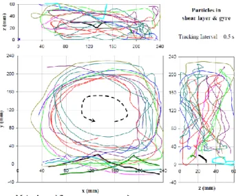
Figure I.29:Particle paths indicating the dynamically active regions of the shear layer and the gyre. (Jamieson and Gaskin,2007) . . . 16

Figure II.1. Photographs of the intersection facility at LMFA . . . .. . . . .19

Figure II.2. Sketch of the cavity geometry: top-view (left) and side-view (right) . . . 20

Figure II.3:The schema for measuring depth . . . 20

Figure II.4: Electromagnetic flowmeters. . . 21

Figure II.5:Classical PIV system, from Brossard (2009) . . . .22

Figure II.6. Cross-correction(Brossard,2009) . . . 23

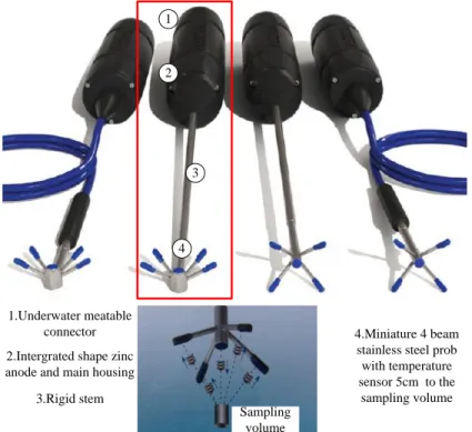
Figure II.7:The different probes and working principle of the side looking probe (Nortek) . . . .25

Figure II.8:Cumulative mean velocity in streamwise and transverse direction . . . . .25

Figure II.9:Application of the Phase-Space Thresholding Method (from Han,2015) .26 Figure II.10: the location for the comparison of ADV and PIV . . . 27

Figure II.11: The comparison of v oscillation signals. . . 27

Figure II.12:The comparison of v oscillation spectrum. . . .28

Figure III.1:Comparison of time-averaged horizontal velocitycomponents among different bed configurations, from Sanjou (2013). . . .31

Figure III.2:Time-Averaged Velocity Vectors, from Kimura (1997). . . . . . .32

Figure III.3:Definition sketch of coordinate system and computed and observed flow velocity in square embayment from Mizumura and Hasatani (2002). . . . .32

Figure III.4:Figure I.9: Measured depth-averaged velocity field, from Booij (1989). . . .33

Figure III.5:The channels of LMFA. . . .. . . ..33

Figure III.6: Horizontal PIV for upstream flow. . . .. . . .. . .34

Figure III.7:Horizontal PIV for upstream flow. . . .. . . .. . . .. . . .35

Figure III.8:Upstream velocity field (the zone from x/L=-0.5 to -1.5). . . .. . . .. . .35

Figure III.9:Upstream velocity field by closing the cavity (the zone from x/L=0.5 to -1.5) . . . .36

Figure III.10:Mean velocity along streamwise direction. . . .. . . .. . . 36

Figure III.11:Horizontal PIV for small cavities. . . .. . . .. . . .. . . 37

Figure III.12:Horizontal PIV for larger cavities. . . .. . . .. . . .37

(14)

List of Figures

Wei CAI, 2015, Experimental study of lateral cavities in open-channel flows XII

Figure III.14:Vertical PIV for lager cavities. . . .. . . .. . .. . . . . . 39

Figure III.15:Measured velocity field in a narrow cavity with two cells for W/L=0.3. . . .. . . .. . .. . . .40

Figure III:16:Measured velocity field in for W/L=0.6. . . .. . . .. . .. . . .. . . ..41

Figure III.17:Measured velocity field in the square cavity with one complete cell for W/L=1. . . .. . . .. . .. . . .41

Figure III.18:Measured velocity field for W/L=1.3. . . .. . . .. . .. . . ..41

Figure III.19:Measured velocity field for W/L=1.7. . . .. . . .. . .. . . ..42

Figure III.20:Cavity with two main cells for W/L=3. . . .. . . .. . .. . . .42

Figure III.21:Large cavity with two cells. . . .. . . .. . .. . . ..42

Figure III.22:Definition of Point 3 and Point 4. . . .. . . .. . .. . . ..43

Figure III.23:Definition of Point 3 and Point 4'. . . .. . . .. . .. . . ..43

Figure III.24:Definition of Point5. . . .. . . .. . .. . . . ..44

Figure III.25:Definition of Point6. . . .. . . .. . .. . . .. . . 44

Figure III.27:Characteristic velocity of main cell. . . .. . . .. . .. . . 45

Figure III.28:Characteristic velocity of the first cell Vc1/Um for all configurations. . .46

Figure III.29:x-position of the center of the cells for all configurations. . . .. . . .. 46

Figure III.30:y-position of the center of main cell for all configurations. . . . .. .. . . .. 47

Figure III.31:y-position of stagnation point for all configurations. . . .. . . .. .. 47

Figure III.32:x-position of stagnation point for all configurations. . . .. . . .. .. 48

Figure III.33:Velocity fields at different elevations for W/L=3. . . .. . . .. . .. . 49

Figure III.34:Velocity fields at different elevations for W/L=4. . . .. . .. . . .. .. .. . 50

Figure III.35:Velocity fields at different elevations for W/L=5. . . .. . . . .. .. .. .. . 51

Figure III.36:Data from Tuna et al. (2013). . . .. . . .. .. .. . . 52

Figure III.37: Velocity fields of second cell region at different transversal locations for W/L=3. . . .. . . .. .. .. . . .. . . 53

Figure III.40:First cells for different geometries with W/L from 1 to 5. . . .. . . . 56

Figure III.41:First cells at different elevations for W/L=3. . . .. . . . .. . . .. . . . 57

Figure III.42:Transition for configurations W/L=2, 2.1, 2.2, 2.3. . . .. . . .. . .. 58

Figure III.43:Streamlines of the flow averaged over 10 seconds, and plotted every 10 seconds for W/L=2. . . .. . . . .. . . .. . . . 58

Figure III.44:Streamlines of the flow averaged over 10 seconds, and plotted every 10 seconds for W/L=2.1. . . .. . . .. . . .. . . . 59

Figure III.47:Flow field averaged over increasing time for W/L=1. . . .. . . 60

(15)

List of Figures

Wei CAI, 2015, Experimental study of lateral cavities in open-channel flows XIII

Figure III.49:Flow field of the second cell averaged over increasing time for

W/L=2. . . 61

Figure III.50:Flow field averaged over increasing time for W/L=3. . . .. . . .62

Figure III.51:Flow field of the second cell averaged over increasing time for W/L=3. . . 62

Figure III.52:Flow field averaged over increasing time for W/L=4. . . .. . . .63

Figure III.53:Flow field of the second cell averaged over increasing time for W/L=4. . . 63

Figure III.54:Mean flow field in every 24 seconds for W/L=5. . . .. . . ..63

Figure III.55 Mean flow field of second cell in every 24 seconds for W/L=5. . . 64

Figure III.56. Velocity field for all configurations. . . 67

Figure IV.1: Scheme of the experimental set-up. . . 73

Figure IV.2:Mean velocity field in the mixing layer along with a few streamlines. . 73

Figure IV.3:(a): Transverse profiles of mean streamwise velocity, (b) and (c): transverse gradient of mean streamwise velocity with white symbols indicating the location of maximum gradient (the spatial resolution is reduced on the right graph for better reading); (d) magnitude of the maximum transverse gradient of mean streamwise velocity.. . . 74

Figure IV.4: (a): streamwise evolution for the outer velocity, the velocity difference and the velocity average. (b): Streamwise evolution of the measured (o) and estimated (*) mixing-layer widths and (c) non-dimensional transverse profiles from (Figure IV.3) of streamwise velocity across the mixing layer.. . . 75

Figure IV.5:(a) spatial distribution of Reynolds shear stress and (b) Transverse profiles of dimensionless Reynolds shear stress at several streamwise locations along the mixing layer... . . .. 76

Figure IV.6:(a) spatial distribution of transverse Reynolds stress and (b) Transverse profiles of dimensionless transverse Reynolds stress at several streamwise locations along the mixing layer.. . . .. . . 76

Figure IV.7: Location of the maximum transverse velocity gradient, Reynolds shear stress and transverse shear stress along the mixing layer.r.. . . .. . . 77

Figure IV.8:Spatial distribution of vorticity in the mixing layer and the cavity.. .. .. .77

Figure IV.9:Spatial distribution of turbulence production in the mixing layer and the cavity.. .. .. . . .78

Figure IV.10: Power spectral density for v(t) plotted for different streamwise locations. A similar scaling is used for all spectrum.. .. .. . . .. .79

Figure IV.11: (a) Streamwise and time evolution of the transverse velocity component along the mixing layer. The capital letters refer to the structures from Figures IV.12 and IV.15. (b) time evolution of u’ and v’ values at y=0 and x/L=0.7.. .. .. . . .80

(16)

List of Figures

Wei CAI, 2015, Experimental study of lateral cavities in open-channel flows XIV

Figure IV.12: Time evolution every 1/3s of fluctuation velocity field (black arrows) averaged over 4 consecutive times (4/30s) and contours of clockwise (blue color, 1<-0.55) and counter-clockwise (red color, 1>0.55) coherent

vortices obtained through POD with the white circle corresponding to the vortex core, that is the maximum local |1|. The dashed line represents the

mixing interface (y=0).. .. .. . . .82 Figure IV.13: Time-evolution of the streamwise location of the clockwise (blue) and

counter-clockwise (red) vortex centers located near the interface (with |y|<50mm). Red arrow corresponds to four periods and equals 6.5s... .. .. . . .. . . . .. . . .84 Figure IV.14: Statistics of spatial location of both types of vortex centers.. . . ... . . . 84 Figure IV.15: Same as Figure IV.12 for other times and other frequency exhibiting

vortices L and M originating from the cavity and ending-up in the mixing-layer. . . .85 Figure IV.16:Mean velocity profiles U/Um along the transverse direction at x/L=0.83

for series 3 and 4 . . . . . . .88 Figure IV.17:Outer velocities U1/Um, U2/Um and ratio r(x) for all configurations from

series 1 and 2 for x/L=0.33 and x/L=0.83 . . . .89 Figure IV.18:Outer velocities U1/Um, U2/Um and ratio r(x) for all configurations from

series 3 (as a function of Re) for x/L=0.33 and x/L=0.83 . . . .. . . ..89 Figure IV.19: Outer velocities U1/Um, U2/Um and ratio r(x) for all configurations from

series 4 for x/L=0.33 and x/L=0.83. . . .89 Figure IV.20: the mixing layer width (x) along the transverse direction for series 3

and 4. . . .90 Figure IV.21: Fit of the linear growth of the mixing layer width. . . 90 Figure IV.22: Fitted linear growth rate of the mixing layer width for all configurations

from series 1 and 2 at x/L=0.33 and 0.83. . . .. .91 Figure IV.23: Fitted linear growth rate of the mixing layer width for all configurations

from series 3 at x/L=0.33 and 0.83. . . .. . . .. . .91 Figure IV.24: Fitted linear growth rate of the mixing layer width for all configurations

from series 4 at x/L=0.33 and 0.83. . . .. . . .. . .92 Figure IV.25:Evolution of the peak frequency normalized by L and Um as a function

of:(a) the aspect ratio of the cavity (W/L) for series 1 (Um=0.167m/s) and

series 2 (Um=0.119m/s); (b): the velocity of the main stream Um and

Reynolds number Re in series 3; (c): the dimensionless water depth h/L in series 4. . . .. . . .. . . .. . . ..93 Figure IV.26: Mean non-dimensional celerity of the vortices in the mixing layer for

all configurations from series 1 and 2. . . .. . . .. . . .. . . .94 Figure IV.27: Mean non-dimensional celerity of the vortices in the mixing layer for all configurations from series 3. . . .. . . .. . . .. . . ..94 Figure IV.28: Mean non-dimensional celerity of the vortices in the mixing layer for

all configurations from series 4. . . .. . . .. . . .. . . ..95 Figure IV.29: Mean non-dimensional wave length in the mixing layerfor all

(17)

List of Figures

Wei CAI, 2015, Experimental study of lateral cavities in open-channel flows XV

Figure IV.30:Mean non-dimensional wave length in the mixing layerfor all configurations from series 3. . . .. . . .. . . .. . . ..95 Figure IV.31:Mean non-dimensional wave length in the mixing layer for all

configurations from series 4. . . .. . . .. . . .. . . ..96

Figure V.1:Mean velocity transverse to the interface between the main stream and the cavity along x axis for W/L=1, 2 ,3,4 and 5. . . .. . . .. . . .. . . ..102 Figure V.2:Scheme of the experimental set-up used for kconc estimation. . . .. . .103

Figure V.3:Calibration = establishing for one pixel the relation between light intensity and scalar concentration. . . .. . . .. . . .. . . .103 Figure V.4:Time-evolution of dye concentration maps for configurations with W/L=1,

red arrows refer to the mean flow direction in the mainstream. . . .104 Figure V.5:Time-evolution of dye concentration maps for configurations with

W/L=3. . . .. . . .. . . .. . . .104

Figure V.6:Time-evolution of dye concentration maps for configurations with

W/L=5. . . .. . . .. . . .. . . .105

Figure V.7:Time-evolution of spatially averaged dye concentration in the cavity for

W/L=1, 3 and 5. . . .. . . .. . . .. . . . . . .. . . .106

Figure V.8:Time-averaged 2D velocity field for W/L=1, 2, 3, 4 and 5. . . . .. . . .108 Figure V.9: Exchange coefficient kveloc estimated for Series 3 as a function of the bulk

velocity and Froude number of the inflow. . . .. .. .109 Figure V.10:Mean velocity transverse to the interface between the main stream and the cavity along x axis for Series 3. . . 109 Figure V.11:Exchange coefficient kveloc estimated for Series 4 as a function of the

dimensionless water depth and Reynolds number of the inflow. . . 110 Figure V.12:Mean velocity transverse to the interface between the main stream and

the cavity along x axis for Series 4. . . 110 Figure V.13: Exchange coefficient as a function of the morphometric parameter from Weitbrecht et al. (2008). . . .. . . 110

Figure A.1from figure III.33. Velocity fields at for W/L=3 for elevations z/h=0.07 (left) and 0.21 (right). . . .. .. . . .. . 117 Figure A.2 from Figure III.4 and III.10: Evolution along the mixing layer of the

mixing layer width and transverse velocity spectrum. . . 117 Figure A.3 from figure III.43:Streamlines of the flow averaged over 10 seconds, and

(18)

List of Figures

Wei CAI, 2015, Experimental study of lateral cavities in open-channel flows XVI

Figure A.4 from figure III.12: Detection of the coherent turbulent structures over time. . . 118 Figure A.5 from figure III.13:Time-evolution of the abscise of the coherent turbulent

structures. . . .. . . .. . . 119 Figure A.6: Data from figures III.16-17-18-56, evolution of the mean 2D-PIV velocity field for increasing aspect ratio of the geometry of the cavity: W/L =0.6, 1, 1.3, 1.6, 1.8. . . .. . . .. . . 119 Figure A.7 from Figure III.30: y-position of the center of main cell for all

configurations. . . .. . . 119 Figure A.8 from Figure III.20:Evolution of the mixing layer width (x) along the

transverse direction as the dimensionless water depth h/L increases. .. . 119 Figure A.9 from Figure III.27: Mean non-dimensional celerity of the vortices in the

mixing layer for all configurations from series 3. . . 121 Figure A.10: Evolution of kveloc coefficient from series as a function of Re (a) and of

(19)

List of Tables

Wei CAI, 2015, Experimental study of lateral cavities in open-channel flows XVII

List of Tables

Table I.1. Range of parameters in previous works. . . .9

Table II.1:Hydraulic conditions used as a reference flow. . . 21

Table III.1: PIV configurations. . . . . . .39

Table III.2:Vertical PIV configurations for different sections. . . .39

Table III.3:PIV configurations for different elevation. . . .40

Table III.4: The parameters of specific points 1, 2, 3, 4 measured at z/h=0.71. . . .45

Table III.5:The estimation time for the stability of the cells. . . .64

Table IV.1:Flow and geometry characteristics, corresponding values of the dimensionless parameters zmeas the altitude at which the velocity profile is measured using the 2D PIV. . . ... . . .. . .87

Table V.1:Flow and geometrical configurations along with k estimated from the literature. . . .. . ... . . .. . . ... . . .. . ..101

Table V.2:Flow and geometrical configurations along with k estimations from the literature with W and L the cavity width and length, h the water depth in the cavity and main stream in front of the cavity, Um the bulk velocity, Re and Fr corresponding Reynolds and Froude numbers in the mainstream, zmeas the altitude at which the velocity profile is measured using the 2D PIV, kveloc and kconc both estimates of the exchange coefficient.. . . . . .. . 107

(20)

List of Tables

(21)

Notations

Abbreviation

ADV Acoustic Doppler Velocimetry

CCD Charge-coupled Device

LMFA Laboratoire de Mecanique des Fluides et Acoustique

PIV Particle Image Velocimetry

POD Proper Orthogonal Decomposition

SNR Signal Noise Ratio

TKE Turbulent Kinetic Energy

W/L The aspect ratio of the cavity

Symbols

Symbol Description Unit

C The mean celerity in the mixing layer [m/s]

f The recording frequency of the camera [s-1]

Fr The froude number [-]

h The depth of the main flow [m]

L The width of the cavity [m]

Ld The total length of the downstream channel [m]

P The turbulent production term [m2_/s3_]

Q The inlet discharge of the main flow [m3/s]

r the outer velocity ratio [-]

R The resolution of the image [m/pixel]

Re The Reynolds number [-]

s The slopes of the upstream and downstream branches of the main channel

[-]

Stk The Stokes number [-]

T The time during the PIV video [s]

Um The mean velocity of the main stream [m/s]

U1 The streamwise velocity measured at the transverse location

in the main flow where the velocity gradient becomes negligibly small

[m/s]

U2 The streamwise velocity measured at the transverse location

in the cavity where the velocity gradient becomes negligibly small

[m/s]

Uex The mean streamwise velocity in the mixing layer [m/s]

u' Fluctuation of streamwise velocity u [m/s]

V1 The velocity at the mid-points between the center of the first

cell and the side wall along X/L=1

[m/s]

V2 The velocity at the mid-points between the center of the first

cell and the cavity interface

[m/s]

Vc1 The characteristic velocity of the first cell [m/s]

(22)

Notations

W The length of cavity [m/s]

x The position along the streamwise direction [m]

xc1 The distance from the center of the first cell to downstream

side wall of the cavity

[m]

xc2 The distance from the center of the second cell to downstream

side wall of the cavity

[m]

x4 The distance from the stagnation point 4 to the downstream

wall of the cavity

[m]

yc1 The distance from the center of the first cell l to the cavity

opening

[m]

yc2 The distance from the center of of the second cell to the cavity

opening

[m]

y3c The distance from the stagnation point 3 to the extremity of

the cavity

[m]

y The position along the transverse direction [m]

z The position along the vertical direction [m]

U The velocity difference [m/s]

t The time period between the two images. [s]

 The coefficient of linear growth rate of the mixing layer width [-]

 Angle between the ADV and the flume reference frames _[◦]

U Rotation angel of principle axis of 2ui and ui [◦]

m The measured width of mixing layer in section x [m]

(23)

Résumé étendu

Chapitre I: Introduction

Le Chapitre d’introduction a pour objectif de présenter les aspects généraux des cavités latérales. Il révèle que les cavités latérales sont une des singularités engendrant une zone de recirculation dans un écoulement permanent, aussi appelée zone d’eau morte. L’écoulement au sein de cette zone de recirculation est d’au moins un ordre de grandeur plus lent que l’écoulement principal et a un débit net nul. De plus, la grande différence de vitesse entre les deux régions donne naissance à une couche de mélange turbulente à l’interface entre ces deux régions. Cette couche de mélange est alors capable de transférer de la quantité de mouvement de l’écoulement principal à la cavité et ainsi de la mettre en mouvement et est aussi capable de transférer des scalaires (gaz, matières solides) entre les deux régions. Du point de vue biologique, les cavités latérales présentent une importance majeure du fait de l’aspect privilégié de cet habitat de faible vitesse mais de constant renouvellement de gaz et matière du fait de sa connexion avec l’écoulement. Les aspects principaux à étudier dans cette thèse sont donc doubles : 1. étudier la forme d’écoulement qui se met en place au sein de la cavité et 2. étudier la capacité de transport de masse entre les deux régions.

Plusieurs types de cavités latérales peuvent être rencontrés dans un écoulement à surface libre, de type rivière, tels que les espaces entre épis, ou les séries de cavités alignées. Dans notre cas, nous nous focaliserons sur les cavités latérales isolées qui correspondent à un élargissement brusque unique de la largeur du canal suivi d’un rétrécissement unique équivalent et qui peut représenter un bras mort, un ancien méandre, un port fluvial ou une zone ouverte sur le côté de l’écoulement (voir Figure. A).

Figure A: Exemple de cavités latérales,( google earth and Lecoz,2007)

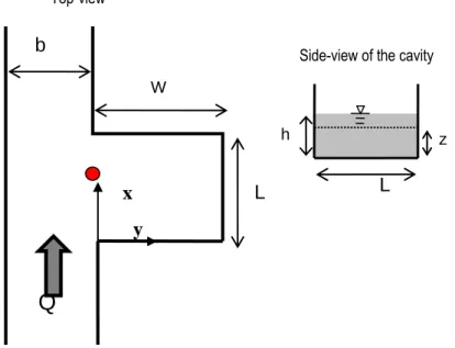
L’approche privilégiée dans la thèse est l’approche expérimentale à échelle réduire considérant une géométrie simplifiée à l’extrême avec une cavité rectangulaire horizontale caractérisée par sa longueur L dans l’axe de l’écoulement et sa largeur W dans la direction perpendiculaire, de la vitesse débitante et de la largeur de l’écoulement principal Um et b respectivement et enfin de la

(24)

Résumé étendu

Figure B:Schéma de la cavité latérale expérimentale

La littérature disponible sur de telles cavités latérales comprend des mesures de champ de vitesse et de transport de scalaire à l’interface. Concernant les champs de vitesse, les auteurs ont principalement étudiées des cavités alignées dans le sens de l’écoulement (W<L) ou carrées (W=L) et ont montré que pour W<<L deux cellules alignées dans l’axe de l’écoulement se développe alors que pour W=L une cellule horizontale occupe l’ensemble de l’espace disponible. Une étude de Booij (1989) a montré que deux cellules alignées dans la direction de W pouvaient être observées pour W=3L. Concernant le transport de scalaire passif, les données de la littérature s’avèrent peu nombreuses et ne permettent pas de conclure quant à l’importance des différents paramètres adimensionnels sur cette capacité de transport, ce qui sera l’objet d’un des chapitres.

Chapitre II: Méthode expérimentale

L’approche choisie pour mener à bien ces travaux est une approche expérimentale sur canal. Le chapitre II présente alors les moyens de mesure utilisés pour mesurer le débit de recirculation, la hauteur d’eau dans la cavité et les champs de vitesse et de concentration dans la cavité. Pour les mesures de vitesse, deux techniques sont utilisés, un ADV permettant de mesurer les 3 composantes de la vitesse localement à haute fréquence et la PIV 2D permettant de mesurer 2 composantes de la vitesse sur un plan rectangulaire à haute fréquence. Tout d’abord, des mesures dans le canal amont permettent de renseigner sur l’état de la couche limite latérale en approche de la cavité. Ensuite, la PIV horizontale est mise en place soit centrée sur la couche de mélange, soit centrée sur la cavité. Dans le cas où deux cellules de recirculation ont lieu dans la cavité, deux champs de PIV sont mesurés, centrés chacun sur une des cellules et une méthode de reconstruction du champs complet est utilisée. Enfin, dans les cas pù l’écoulement est fortement 3D, des plans de PIV verticaux sont mesurés et permettent de mieux appréhender la forme de l’écoulement.

Chapitre III: Formes d’écoulement dans la cavité

Pour ce chapitre, une configuration d’écoulement dite « de référence » est définie et les vitesses amont et hauteur d’eau sont conservées fixé tout au long du chapitre. Le seul paramètre que l’on fait alors varier est le rapport d’aspect géométrique horizontal de la cavité W/L. Pour chaque valeur de

W/L, une mesure PIV est réalisée à z/h=0.71 de la façon détaillée au chapitre II.

-Tout d’abord, pour 0.6<W/L<2, une cellule unique, appelée 1ère cellule, occupe l’ensemble de l’espace disponible (Figure. C), à l’exception de petites cellules contra-rotatives cantonnées dans les coins. Cette cellule est donc de dimensions proches de W*L et a déjà été observée dans la littérature.

U

m b L L W y x h

Side-view of the cavity Top-view

(25)

Résumé étendu

-Pour 2W/L<2.3, une deuxième cellule de plus petite taille prenant naissance au coin (x=W, y=L)

tend à grandir et occuper une plus grande partie de la largeur de la cavité x/L à mesure que W/L augmente (Figure. C). Des mesures additionnelles (voir Figure. D) ont montré que les configurations W/L=2 d’une part et 2.3 d’autre part, sont stables dans le temps alors que les configurations intermédiaires W/L=2.1 et 2.2 sont instables et oscillent entre i) une configuration d’écoulement où la 2e

cellule est confinée au coin (comme pour W/L=2) et une configuration où cette 2e cellule occupe l’ensemble de la largeur disponible (comme pour W/L=2.3). La valeur de

W/L=2.2-2.3 est alors définie comme la transition entre zone de recirculation à 1 cellule et à 2

cellules.

-Pour 2.3W/L3, deux cellules prennent place, l’une à côté de l’autre alignées suivant x, confirmant ainsi la mesure de Booij (1989) dans la littérature (Figure. C).

-Enfin, pour W/L>3, l’écoulement au-delà de la 1ere cellule devient fortement 3D et beaucoup plus complexe. La méthode de PIV 2D montre alors ses limites pour caractériser l’écoulement.

Maintenant, concernant la dimension des cellules, la Figure. C montre que:

-Pour W/L<2.2 l’extension de la 1ère cellule augmente à mesure que W augmente de telle sorte que cette extension reste égale à W.

-Pour W/L passant de 2.1 à 2.2, la dimension de la 1ere cellule diminue subitement de 2.1L à 1.7L et la 2e cellule grandit et occupe, pour W/L=2.2, les x=0.5L restant. Ensuite, pour 2.3W/L<3,

l’extension de la 1ère

cellule ne varie plus et reste égale à environ 1.7L alors que la 2e cellule occupe l’espace disponible et sa dimension augmente donc à mesure que W augmente.

-Enfin pour W/L>3, l’écoulement dans la 2e cellule devient fortement 3D et les dimensions telles qu’introduites ci-dessus perdent du sens.

Enfin, concernant la vitesse de l’écoulement au sein de ces cellules, la Figure. C montre qu’au sein de la 1ère cellule, la vitesse de rotation n’évolue que très peu à mesure que W augmente et vaut de l’ordre de 2cm/s soit de la vitesse débitante de l’écoulement principal. Il apparaît ainsi que la zone en noire (correspondant à une vitesse supérieure à 2.75cm/s) est mesurée pour W/L=0.6 à 5. En conséquence, les deux vitesses extérieures bordant la couche de mélange restent à peu près identiques. Cela explique le résultat du chapitre 4 où la capacité de transfert de masse ne varie quasiment pas lorsque W varie. Ensuite, la vitesse de la 2e cellule est nettement inférieure à celle de la 1ere, avec une vitesse caractéristique de l’ordre de 0.5cm/s pour W/L3, correspondant à un rapport de vitesse de 1/4 par rapport à la 1ère cellule et de l’ordre de 0.2cm/s (rapport de 1/10) pour

(26)

Résumé étendu

Figure C:Champs de vitesse moyenne 2D horizontal mesuré dans la cavité par PIV à l’élévation 0.71h pour différentes géométries où W/L varie.

W/L=0.3 W/L=0.6 W/L=1 W/L=1.3 W/L=1.6 W/L=1.7 W/L=1.8 W/L=1.9 W/L=2 W/L=2.1 W/L=2.2 W/L=2.3 W/L=2.6 W/L=3 W/L=3.3 W/L=3.6 W/L=4 W/L=4.3 W/L=4.6 W/L=5

(27)

Résumé étendu

Figure D:Lignes de courant du champ de vitesse 2D horizontal mesuré toutes les 10s et moyenné chacun sur 10s, pour la configuration W/L=2.2

Chapitre IV: Couches de mélange

Le chapitre IV présente le fait qu’à l’interface entre l’écoulement principal et la cavité, une intense couche de mélange a lieu du fait du fort gradient de vitesse entre ces deux régions. Cette couche de mélange (le long de l’axe x comme montré sur la Figure E.a) est contrainte entre les deux arrêtes situées à x=0 et x=b et il apparaît que l’axe de la couche de mélange, défini comme la position de maximum gradient transverse (selon y) de vitesse longitudinal (selon x), suit à peu près le segment reliant ces deux coins (voir Figure E.b et E.c), c’est-à-dire l’axe x lui-même.

a

b c

Figure E:Schéma de la cavité latérale carrée à surface libre (y>0) et de l’écoulement principal (y<0) adjacent (a). Evolution longitudinale (selon x) : des profils transverse (selon y) de vitesse moyenne

longitudinale (b), de gradient transverse de cette vitesse (c),

Ainsi, l’axe de la couche de mélange est contraint par la configuration géométrique et à son extrémité aval (x/b=1), la couche de mélange impacte le coin aval. Ces deux spécificités associées à

(28)

Résumé étendu

la géométrie de la singularité modifient les caractéristiques de la couche de mélange par rapport à une couche de mélange classique libre de toute paroi, comme détaillé ci-dessous :

-L’épaisseur de la couche de mélange augmente à peu près linéairement jusque vers x/b=0.8 mais diminue soudainement sur sa partie aval (Figure F.a).

-La contrainte de Reynolds de cisaillement horizontal normalisée par la différence des vitesses moyennes externes (U1 mesurée dans la cavité et U2 dans l’écoulement principal), augmente

d’amont en aval, atteint un maximum vers x/b=0.7 puis diminue en s’étalant transversalement (Figure F.b), en lien avec la réduction soudaine de l’épaisseur de couche de mélange.

a b

Figure F:Evolution longitudinale (selon x) : de l’épaisseur  de la couche de mélange (a) et des profils de contrainte turbulentes de cisaillement horizontal (b).

-Le spectre d’énergie de la vitesse transverse (selon y) montre (Figure G.a) que sur sa portion amont (x/b<0.5), la bande de fréquence de passage des structures turbulentes est assez étalée alors qu’entre

x/b=0.5 et 0.6, cette bande se resserre sur une fréquence pic (égale à 0.58Hz dans le cas présent) ;

on peut dire que la couche de mélange « s’organise » le long de son axe de développement. Plus à l’aval, entre x/b=0.6 et 0.8, ce pic de fréquence est maintenu, mais à l’approche du coin aval, la couche de mélange tend à se désorganiser et à perdre toute énergie.

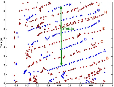
-Ce pic à f=0.6Hz est retrouvé sur la Figure G.b où la vitesse transverse instantanée (v, selon y) est tracée le long de la couche de mélange (x/b, en abscisse) au cours du temps (t, en ordonnées). Cette figure permet de visualiser l’alternance de vitesse dirigée de l’écoulement vers la cavité (v>0 en jaune-orange) et de la cavité vers l’écoulement (v<0 en bleu). Dans la zone organisée (x/b>0.5), cette alternance correspond à l’alternance de passage des structures turbulentes (voir Figure G.b). La flèche rouge couvrant 4 périodes mesure environ 6.5s, ce qui confirme la fréquence de passage de 0.6Hz.

-La Figure G.c présente i) en flèches noires les champs de vitesse instantanés tracés tous les 1/3 de secondes et ii) en couleur les isovaleurs de 1 définit par Graftieux et al. (2001), correspondant à la

zone centrale des structures de rotation horaire en bleu et anti-horaire en rouge. Il apparaît, de plus, que les zones de forte vitesse transverse sur la Figure G.b correspondent aux zones situées entre ces centres de structures alors que la Figure H présente la position longitudinale de leur centre où il apparaît que le leur célérité est relativement constante et que leur fréquence de passage vaut bien ~0.6 Hz. La Figure G.c montre que les centres de ces structures cohérente ne se trouvent pas sur l’axe de la couche de mélange mais plutôt décalés vers la cavité ou l’écoulement principal et que deux organisations principales sont observées : i. les cellules bleues (sens horaire) dans la cavité et les rouges (sens anti-horaire) dans l’écoulement principal (tel à t=1.9s) ou ii. l’opposé (tel à t=6.2s). Au final, la couche de mélange à l’interface de la cavité révèle une alternance de 4 phases consécutives : 1. une forte vitesse transverse dirigée vers la cavité, 2. une cellule cohérente de sens de rotation horaire, 3. une forte vitesse transverse dirigée vers l’écoulement principal et 4. une cellule cohérente de sens de rotation anti-horaire. Cette organisation très périodique de structures cohérentes et de zones de vitesse transverse permettra de mieux comprendre la capacité de transport de scalaire entre la cavité et l’écoulement principal.

(29)

Résumé étendu

a b

c

Figure G:Evolution longitudinale des spectres d’énergie de la vitesse transverse (a). Evolution spatio-temporelle de la norme de vitesse transverse instantanée (b). Champs de vitesses chaque 1/3s

(30)

Résumé étendu

Figure H:Evolution spatio-temporelle de la position longitudinale des centres des cellules cohérentes identifiées sur le graphique h (d).

Chapitre V: Echange de masse entre les deux régions

Dans le chapitre V, le dispositif expérimental est adapté pour l’étude des échanges de scalaire passif entre la cavité et l’écoulement. Dans un premier temps, seul l’eau claire recirculante est utilisée et l’écoulement dans la cavité se met en place. A un instant donné, un débit faible mais très concentré en colorant (alimentaire ici) est injecté à débit constant à l’amont de l’écoulement amont de façon à optimiser son homogénéisation, comme montré sur la Fig. Ia. Lorsque le colorant entre dans la cavité, des photographies sont prise depuis le dessus de la surface libre et grâce à une calibration antérieure, les champs de concentration peuvent être reconstruits, comme présenté sur la Figure I.b pour une cavité carrée (W/L=1) et Ic pour une cavité rectangulaire (W/L=3). Il apparaît que dans un premier temps les processus associés à ce transfert sont identiques. Les structures cohérente présentes dans la couche de mélange permettent un transfert turbulent de colorant tout au long de la couche de mélange de l’écoulement vers la cavité (t~5s sur Figure I.b-c). Ce colorant est alors advecté par la cellule de recirculation vers le coin aval où cette concentration augmente puis le long de la paroi aval de la cavité (t~10s), puis tout le long de la zone externe de la première cellule de recirculation (celle située le plus à gauche au contact avec l’écoulement). Ainsi vers t~20s pour la cavité carrée ou t~35s pour celle rectangulaire, l’ensemble de la couche externe de la première cellule est colorée et le colorant se trouve en contact avec l’écoulement près du coin amont. Le fait que ce temps soit plus court pour la cavité carrée est due au fait que la vitesse est légèrement supérieur et que l’extension de cette cellule est plus faible pour la cavité carrée que pour celle rectangulaire (Figure C). Dans le même temps, la diffusion turbulente permet un transfert de colorant de la couche externe vers le centre de la cellule où la concentration augmente lentement. De plus pour le cas de la cavité rectangulaire, une part du colorant de la première cellule rejoint la deuxième cellule (t~80s sur la Figure I.c), qui met donc beaucoup plus de temps à se polluer, du fait aussi de sa faible vitesse d’advection et faible niveau de turbulence.

(31)

Résumé étendu

Figure I: Schéma de la cavité modifiée pour étudier le trasnport de scalaire de l’écoulement principal vers la cavité (a). Champs de concentration de scalaire au cours du temps pour la cavité

carrée (W/L=1) (b) et la cavité rectangulaire (W/L=3) (c).

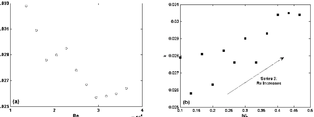
Ces travaux permettent enfin de calculer un coefficient de transfert du scalaire de l’écoulement principal (noté k) vers la cavité qui s’avère être identique pour les deux géométries de cavité. L’analyse dimensionnelle révère que dans notre configuration simplifiée, en régime fluvial et lisse, 3 paramètres sont susceptibles d’affecter ce coefficient k : la forme géométrique de la cavité W/L, la hauteur d’eau normalisée h/L et le nombre de Reynolds de l’écoulement amont Re. Tout d’abord il s’avère pour deux écoulements que la géométrie de la cavité W/L n’a que très peu d’effet sur k. De plus, la Figure J.a montre que lorsque Re augmente, k diminue à peu près linéairement, alors que la Figure J.b montre que lorsque h/L augmente (ainsi que Re), k augmente à peu près linéairement. Cela révèle que k tend à augmenter lorsque Re décroit ou h/L augmente et que l’effet de h/L domine celui de Re dans la gamme des paramètres étudiés.

b=0.3m b 2m 2m b=0.3m L 2m 2m W Q h Dye release t=5s t=10s t=20s t=35s t=55s t=80s t=105s t=130s t=5s t=20s t=35s t=80s t=130 s t=180s a b c b=0.3m b 2m 2m b=0.3m L 2m 2m W Q h Dye release t=5s t=10s t=20s t=35s t=55s t=80s t=105s t=130s t=5s t=20s t=35s t=80s t=130 s t=180s a b c

(32)

Résumé étendu

Figure J:Evolution du paramètre k en fonction du nombre de Reynolds Re (a) et de la hauteur d’eau normalisée h/L (b, avec Re qui augmente lorsque h/L augmente).

(33)

Chapter I: Introduction

The aim of this Chapter is to give an overview of main researches on the open-channel lateral cavities, focusing on the main three aspects considered in this work i.e. the studies of flow patterns in the cavity, of the mixing layer at the interface with the main stream and of the mass transfer between the two regions.

Chapter I:Introduction ... 1

1 Dead zones in river flow ... 3 2 Lateral cavities ... 5 3 Mixing layer ... 11 4 Mass transfer ... 14 5 Scientific issue and organization of the manuscript... 16

(34)

(35)

1 DEAD ZONES IN RIVER FLOW

A river flow is a complex watercourse including portions where the flow is rapid, almost 1D directed towards downstream parallel to the main axis of the river and zones of complex flow patterns where the flow direction is varying spatially. Among these zones are the so-called “dead zones” that are defined as volumes, either aligned along a vertical or horizontal axis, where the integral of the mean discharge is nil, so that this portion of the river does not participate to the river discharge capacity. These dead zones thus exhibit streamwise velocities oriented towards upstream and towards downstream that cancel each other so that the net discharge is nil. These zones of complex flows are usually created by singularities in the river topography or artificial structures. These dead zones are either naturally present in the flow, downstream boulder or macro-roughness (see for instance Mignot et al., 2009 or Franca, 2005), downstream islands (see for instance Babarutsi et al., 1989), in a bifurcation (see Mignot et al., 2014 and Figure I.2) or a junction (see Shakibainia et al., 2010 and Figure I.3), downstream a flow enlargement (see Babarutsi et al., 1989 – Figure I.1 below – and Han, 2015), etc. They can also be a consequence of an artificial structure added to the river, reviewed by Li and Djilali (1995) in Figure I.4, such as a bridge pier (see for instance Chen and Jirka, 1995 and Figure I.5) a groyne or dike (see Peltier et al., 2013 and Figure I.6), around an obstacle (Hattori and Nagano, 2010 and Figure I.7). Among these dead zones are the cavities, which can be defined as an area connected to a main stream through one face, with a free surface and closed along the 3 other sides and that we will detail in the sequel.

These dead zones are of major importance for the river biology and chemistry activity (see Lecoz, 2007) as they are areas with velocities of about one order of magnitude lower than the main stream but still connected to the main stream. Fauna and Flora can thus encounter there a location to rest where the concentration of gazes, nutriments etc. remains high thanks to the exchanges with the adjacent main stream through a turbulent mixing layer. These areas are thus of primary importance for the river restoration programs (see for example Klein et al., 1994 for a French example).

Figure I.1:Shallow Open Channel Flow downstream a sudden Channel Expansion, from Babarutsi et al. (1989)

(36)

Figure I.2. Velocity magnification to unveil the recirculation region from Mignot et al. (2014)

Figure I.3: Conceptual model of separation zone in channel confluences from Shakibainia et al. (2010)

(37)

Figure I.5: shallow near-wake flow pattern produced by cylinder: unsteady bubble wake with weaker downstream instabilities, from Chen and Jirka (1995)

Figure I.6:Two-dimensional depth-averaged velocity fields for flow-cases (Peltier et al. ,2013)

Figure I.7:Streamlines around the step, from Hattori (2010)

Figure I.8:Interpretation of the investigated flow field, from Franca (2005)

2 LATERAL CAVITIES

Two main types of cavities can be encountered: a) “closed-conduit cavities”, thus without free-surface, bounded by walls and a connection with the main stream; the cavity may be located either on the side, top or underneath the main stream and b) the “open-channel cavities”, thus with a free surface, connected to the main stream through a lateral face, and comprised within three lateral and

(38)

a bottom wall plus the free surface above. The main difference between both types lies in the existence or not of a free surface and thus of a vertical confinement of the cavity flow. "Open-channel cavities" are generally referred to as "lateral cavities" or "side cavities".

Lateral cavities consist of a relatively large volume of water initially located on the side of a main flow of relatively high speed. These lateral cavities can themselves be divided into: A. the isolated cavities (as in the present case), B. the cavities located between two consecutive groins (see Uijttewaal et al., 2001 and Figure I.9) and C. the series of lateral cavities (see Erpicum et al., 2009 and Figure I.10). Differences between these configurations mainly lie in the direction of the main stream velocity as reaching the upstream limit of the cavity. Unlike case A, in cases B and C the transverse velocity of the main stream is not nil when reaching the studied cavity ; it is directed towards the main stream as it is influenced by the flow leaving the upstream cavity. Moreover, coherent turbulent structures originating from upstream cavities or groynes influence the flow. Literature on groyne fields focuses more on the number of recirculation cells and the exchanges between the main stream and the cavity. Such experiments are proposed by Langendoen et al. (1994), Uijtewaal et al. (2001), Weitbrecht et al. (2008, see Figure I.11). They show that, compared to a single cavity, the groyne fields are characterized by the interaction between the successive cavities. Recent numerical contributions are the ones of Hinterberger et al. (2007) and McCoy et al. (2008), the latter emphasizing on the three-dimensionality of the flow in the cavity.

Figure I.9:Schematized Top View of Shallow Flume with Five Groyne Fields Adjacent to Main Stream, from Uijttewaal et al. (2001)

Figure I.10:Plane view of the test flume (above) and definition of the parameters of the macro-rough geometrical configurations (below), from Erpicum et al. (2009)

(39)

Figure I.11. Schematic of the idealized groin field model, from Weitbrecht et al. (2008) The present paper is dedicated to lateral cavities of type A, which are encountered in various open channel flow hydrodynamics situations. Oxbows, cut-off meanders are natural isolated lateral cavities connected to rivers while harbors connected to a river or sea streams are typical artificial isolated lateral cavities. In the fluvial environment, these situations correspond to meanders (Figure I.12a); to old dead rivers channels (Figure I.12b) or spacing ears positioned perpendicularly to the banks; to river ports (Figure I.12d) where the artificial socket is then connected to the adjacent stream. In the coastal environment, the cavity is generally a port (Figure I.12c), connected to the sea in which a coastal current parallel to the coast develops.

Figure I.12. Lateral cavities,from google earth and Lecoz (2007)

Contributions concerning lateral cavities mix experimental (based on PIV measurements) and numerical approaches (Kimura and Hosoda, 1997; Nezu et al., 2002 ; Mizumura and Yamasaka, 2002). Kodotani et al. (2008) measured simultaneously the velocity field at the surface and surface level oscillations to correlate seiching and streamwise velocity in the main stream.

When focusing on the recirculation cells (often referred to as “recirculations” throughout manuscript) that develop in the cavity, the main parameter emerging from literature is the aspect ratio W/L of the cavity with W the cavity width (along the crosswise direction, perpendicularly to the main stream direction) and L its transverse dimension. Most studies in the literature consider a low aspect ratio (W/L1)

1. For W/L<<1, two cells are observed, aligned in the streamwise direction, as for instance in Sanjou and Nezu (2013).

(40)

Figure I.13:Comparison of time-averaged horizontal velocity components among different bed configurations, from Sanjou and Nezu (2013)

2. For W/L1, a single quasi 2D recirculation cell occupies the whole cavity, as for instance in Mizumura and Kimura (2002)

Figure I.14:Time-Averaged Velocity Vectors:Definition sketch of coordinate system and computed and observed flow velocity in square embayment. From Mizumura and Kimura (2002)

(41)

Figure I.15. Time-Averaged Velocity Vectors, from Kimura and Hosoda (1997)

3. For W/L>1, only one contribution was encountered: the work by Booij (1989) where two cells are observed. Note that for a groyne field, Weitbrecht et al. (2008)’s experiments, with W/L reaching 2, also obtained a second recirculation.

Figure I.16:Measured depth-averaged velocity field, from Booij (1989)

Figure I.17: Mean flow properties in groin field flows with aspect ratios W/L=2, where the 2-gyre systems are visible, from Weitbrecht et al. (2008)