HAL Id: hal-01724972
https://hal.archives-ouvertes.fr/hal-01724972
Submitted on 1 Apr 2019HAL is a multi-disciplinary open access archive for the deposit and dissemination of sci-entific research documents, whether they are pub-lished or not. The documents may come from teaching and research institutions in France or abroad, or from public or private research centers.
L’archive ouverte pluridisciplinaire HAL, est destinée au dépôt et à la diffusion de documents scientifiques de niveau recherche, publiés ou non, émanant des établissements d’enseignement et de recherche français ou étrangers, des laboratoires publics ou privés.
Typology of the flow structures in dividing open channel
flows
Adrien Momplot, Gislain Lipeme Kouyi, Emmanuel Mignot, Nicolas Rivière,
Jean-Luc Bertrand-Krajewski
To cite this version:
Adrien Momplot, Gislain Lipeme Kouyi, Emmanuel Mignot, Nicolas Rivière, Jean-Luc Bertrand-Krajewski. Typology of the flow structures in dividing open channel flows. Journal of Hydraulic Research, Taylor & Francis, 2017, 55 (1), pp.63-71. �10.1080/00221686.2016.1212409�. �hal-01724972�
Typology of the flow structure in dividing open channel flows
1
ADRIEN MOMPLOT1, GISLAIN LIPEME KOUYI1, EMMANUEL MIGNOT2, NICOLAS
2
RIVIERE2, JEAN-LUC BERTRAND-KRAJEWSKI1
3 4
1 Université de Lyon, INSA de Lyon, LGCIE – Laboratory of Civil & Environnemental Engineering, 5
F-69621 Villeurbanne cedex, FR Emails: [email protected] (Corresponding Author);
6
[email protected]; [email protected] 7
8
2 LMFA, CNRS-Université de Lyon, INSA de Lyon, Bât. Joseph Jacquard, 20 Avenue Albert Einstein, 9
F-69621 Villeurbanne cedex, FR Emails: [email protected]; [email protected]
10 11
ABSTRACT
12
The present study reports the occurrence of a new recirculation structure taking place in the lateral
13
branch of a 90° bifurcation flow. This recirculation structure is “helix-shaped” and strongly differs
14
from the typical “closed” recirculation often reported in the literature. The aim of the study is to detail
15
their characteristics using experimental and numerical approaches and to establish a typology, i.e. the
16
flow conditions leading to each recirculation structure based on the upstream Froude number and the
17
upstream aspect ratio.
18
Keywords: bifurcation, hydraulic parameters, open-channel flow, RANS model, recirculation
19
structures 20
1 Introduction 21
Bifurcations of open-channel flows are specific structures frequently encountered in sewer 22
systems or river delta. Bifurcation flows have been widely studied (Grace and Priest, 1958; 23
Shettar and Murthy, 1996; Hsu et al., 2002; Ramamurthy et al., 2007; Mignot et al., 2013; 24
Momplot et al., 2013). Hence, governing parameters of a bifurcation flows are well identified: 25
inlet discharge and discharge repartition in downstream channels. In the literature, the 26
principal challenge for bifurcations lies in the prediction of the flow distribution from the 27
incoming flow towards each outgoing flow. A review of analytical models developed to 28
access such prediction can be found in Rivière et al. (2007, 2011). The model proposed by the 29
authors is based on the momentum conservation law as proposed by Ramamurthy et al. 30
(1990), suitable stage-discharge relationships for the downstream controls in the outflow 31
channels and an empirical correlation obtained through experimental data. 32
Nevertheless, understanding the behavior of the flow structures within the bifurcation 33
is also important, as they strongly impact pollutant or sediment transport and mixing 34
processes. The general pattern of a steady subcritical 3-branch bifurcation is described by 35
Neary et al. (1999). A three-dimensional recirculating region develops in the lateral branch 36
and secondary flows appear in both outlets. Mignot et al. (2014) detailed the mixing layer 37
taking place at the frontier between the main flow and the recirculation zone in the lateral 38
branch. Recirculation zones, also defined as bubbles, are encountered in various geometries as 39
listed by Li and Djilali (1995). 40
Regarding specifically the recirculation zone, authors such as Kasthuri and 41
Pundarikanthan (1987), Shettar and Murthy (1996) and Neary et al. (1999) sketch the 42
recirculation zone (in top view) as a closed semi-elliptic region developing along the 43
upstream wall of the lateral branch with maximum length and width at the free-surface and 44
minimum extensions in the near-bed region. Kasthuri and Pundarikanthan (1987) and Shettar 45
and Murthy (1996) respectively measure and compute the free-surface length and width of 46
this recirculation zone. The authors agree that as the relative lateral discharge increases, the 47
dimensions of the recirculation zone decreases. Neary et al. (1999) then compute flow 48
configurations with varying channel width ratios and dimensionless water depths and exhibit 49
varying characteristics of the recirculation zone pattern without clear explanation of the 50
different types of recirculation zones. 51
The aim of the present paper is twofold: first to describe the two main flow structures 52
that can be observed in the lateral branch of a 90° bifurcation and second to determine the 53
flow conditions for which each structure is observed. The paper is organized as follows: after 54
presenting the experimental and numerical approaches, the characteristics of the different 55
types of recirculation zones are described based on two measured and computed flows (F1 56
and F2) and finally a campaign of numerical simulations (including 16 different cases) is led 57
in order to establish the flow typology. 58
2 Material and methods 59
2.1 Experimental set up
60
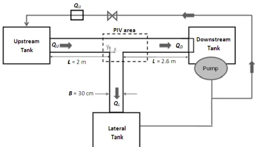
The experimental set-up (see Fig. 1) is a horizontal 3-branch equal width (B=30 cm) glass 61
open-channel bifurcation of 2 and 2.6 meters long channels for the inlet and both outlet 62
respectively. Boundary conditions are the inlet discharge QU (measured by a flow-meter in the 63
pumping loop) and the weir crest height CD and CL at the downstream end of each of the two 64
outlet channels. The water depths in the upstream, lateral and downstream branches are 65
defined as hU, hL and hD respectively and are measured using a digital point gauge. The 66
discharge distribution QL/QU in the bifurcation is measured through an additional flow-meter 67
in the pumping loop. In the studied cases, flow conditions are sub-critical everywhere. Details 68
about this set-up are available in Mignot et al. (2013 and 2014). 69
70
71
Figure 1. Experimental set up used for flow validation. 72
2.2 Modelling strategy
73
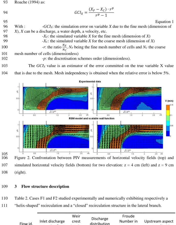
Numerical simulations are performed under the commercial software ANSYS Fluent version 74
14.0, following the modelling strategy proposed by Momplot et al. (2013) for computing 75
bifurcation flow F0 (see Table 1), these simulations are confronted with PIV measurements of 76
the horizontal velocity fields (see Fig. 2). Overall performances are fair. Additionally, 77
simulated discharge repartition and measured discharge repartition shows fair agreement 78
(differences are less than 10%). 79
Table 1. Characteristics of the validated flow. 80 Flow id. Inlet discharge QU (L.s-1) Weir crest height hcrest (m) Discharge distribution (QL/QU) Froude Number in upstream channel (-) Upstream aspect ratio B/hU (-) F0 4 0.12 0.51 0.102 2.5 81
The model solves the RANS (Reynolds Averaged Navier-Stokes) equations using the 82
Volume of Fluid - VOF -method for computing the free-surface curve and a Reynolds stress 83
model - RSM - as turbulence model for system closure (see Launder et al., 1975). Scalable 84
wall-functions (see Grotjans and Menter, 1998) are used for walls; a uniform velocity UInlet is 85
set at the inlet cross-section; atmospheric pressure P0 is set at the top of the computational 86
domain and at outlets. Crest heights are explicitly represented in the mesh. After the weirs, 87
standard pressure outlet conditions are set. Discretisation scheme use for pressure is Body-88
Force Weighted and Second-Order Upwind for other variables. Pressure-velocity coupling
89
algorithm is PISO. 90
Mesh independency is verified using the grid convergence index (GCI) defined by 92 Roache (1994) as: 93 𝐺𝐶𝐼𝑋 = (𝑋𝐹− 𝑋𝐶) ∙ 𝑟𝑝 𝑟𝑝− 1 94 Equation 1 95
With : -GCIX: the simulation error on variable X due to the fine mesh (dimension of 96
X), X can be a discharge, a water depth, a velocity, etc.
97
-XF: the simulated variable X for the fine mesh (dimension of X) 98
-XC: the simulated variable X for the coarse mesh (dimension of X) 99
-r: the ratio 𝑁𝐹
𝑁𝐶, NF being the fine mesh number of cells and NC the coarse
100
mesh number of cells (dimensionless) 101
-p: the discretisation schemes order (dimensionless). 102
The GCIX value is an estimator of the error committed on the true variable X value 103
that is due to the mesh. Mesh independency is obtained when the relative error is below 5%. 104
105
Figure 2. Confrontation between PIV measurements of horizontal velocity fields (top) and 106
simulated horizontal velocity fields (bottom) for two elevation: z = 4 cm (left) and z = 9 cm 107
(right). 108
3 Flow structure description 109
Table 2. Cases F1 and F2 studied experimentally and numerically exhibiting respectively a 110
“helix-shaped” recirculation and a “closed” recirculation structure in the lateral branch. 111
Flow id. Inlet discharge
QU (L.s-1) Weir crest height hcrest (m) Discharge distribution (QL/QU) Froude Number in upstream channel (-) Upstream aspect ratio B/hU (-) F1 8 0.09 0.47 0.218 2.50 F2 4 0.025 0.50 0.448 6.69 112 113
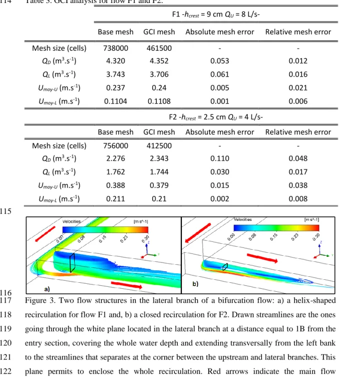
Table 3. GCI analysis for flow F1 and F2. 114
F1 -hcrest = 9 cm QU = 8 L/s-
Base mesh GCI mesh Absolute mesh error Relative mesh error
Mesh size (cells) 738000 461500 - -
QD (m3.s-1) 4.320 4.352 0.053 0.012
QL (m3.s-1) 3.743 3.706 0.061 0.016
Umoy-U (m.s-1) 0.237 0.24 0.005 0.021
Umoy-L (m.s-1) 0.1104 0.1108 0.001 0.006
F2 -hcrest = 2.5 cm QU = 4 L/s-
Base mesh GCI mesh Absolute mesh error Relative mesh error
Mesh size (cells) 756000 412500 - -
QD (m3.s-1) 2.276 2.343 0.110 0.048 QL (m3.s-1) 1.762 1.744 0.030 0.017 Umoy-U (m.s-1) 0.388 0.379 0.015 0.038 Umoy-L (m.s-1) 0.211 0.21 0.002 0.008 115 116
Figure 3. Two flow structures in the lateral branch of a bifurcation flow: a) a helix-shaped 117
recirculation for flow F1 and, b) a closed recirculation for F2. Drawn streamlines are the ones 118
going through the white plane located in the lateral branch at a distance equal to 1B from the 119
entry section, covering the whole water depth and extending transversally from the left bank 120
to the streamlines that separates at the corner between the upstream and lateral branches. This 121
plane permits to enclose the whole recirculation. Red arrows indicate the main flow 122
directions. 123
124
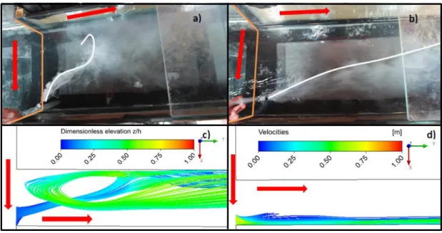
Figure 4. Laboratory and simulation observations of two different flow structures in the 125
lateral branch of two bifurcation flows: F1 (a-c) and F2 (b-d). (a-b) show experiments, (c-d) 126
show numerical streamlines colored by the dimensionless elevation z/hL (from blue, being the 127
bottom of the channel; to red, being the free-surface). For (a-b), a white dye tracer is injected 128
in the downstream corner of the lateral channel, near the bottom, the white line represents the 129
limit of the tracer extension, red arrows indicate flow directions and orange lines mark the 130
inlet section of the lateral branch. 131
132
Among all studied flows, two recirculation structures could be observed. Table 2 presents two 133
flow cases investigated numerically and experimentally, each one exhibits a different 134
recirculation structure: a so-called “helix shaped” for F1 and a “closed” one for F2. Fig. 4 135
shows numerical results for these flow cases and particularly the behaviour of some selected 136
streamlines. Fig. 4 compares experimental observations for the two flow cases regarding the 137
transport of white dye tracer in the lateral branch and numerical streamlines obtained through 138
RANS simulations. In both cases, injection takes place near the bottom part of the 139
downstream corner region. These results confirm the fair agreement between simulated and 140
measured flow patterns. Additionally, results of the GCI analysis displayed in Table 3 141
indicates that meshes used to compute both flows are efficient for the prediction of discharge 142
and bulk velocities in the lateral branch. Surprisingly, the mesh for flow F2 is less efficient 143
for discharge and velocities representation in the upstream branch than the mesh for flow F1. 144
The two figures permit to describe both recirculation structures: 145
- The closed recirculation observed for flow F2 is a 2D semi-elliptic closed region 146
developing along the upstream wall of the lateral branch as described in the literature: no flow 147
enters or leaves this region and it is of larger streamwise and transverse extension at the free-148
surface than near the bed (Fig. 3b). Consequently, the streamlines starting from the 149
downstream corner of the intersection remain quite parallel to the banks of the lateral channel 150
towards downstream and do not interact with the recirculation zone (Fig. 4b). 151
- The helix-shaped recirculation observed for flow F1 is a 3D ascendant flow (see Fig. 152
3a and 4c): i. supplied by the bottom flow of the upstream channel, ii. entering the lateral 153
branch near the bottom part of the downstream corner area, iii. approaching the opposite 154
(upstream) wall of the lateral branch, iv. raising towards the free-surface, first in the direction 155
of the intersection (towards upstream) and then towards downstream along center of the 156
branch. v. escaping towards downstream in the upstream half of the branch. Consequently, the 157
streamlines starting from the downstream corner of the intersection enter the recirculation 158
structure (Fig. 4a). These two distinct flow structures corroborate the different streamlines 159
plots near the bottom reported by Neary et al. (1999) in their figure 10 and the pathlines in 160
their figure 11c. 161
4 Flow typology 162
In order to establish the flow conditions for which each recirculation structure is observed, a 163
flow typology is established following the parameters obtained through dimensional analysis. 164
Using the same approach as Mignot et al. (2013) and assuming (as for the authors) that the 165
flow is turbulent (see Table 10) and smooth, the 8 parameters governing the flow 166
characteristics are: the three discharges (QU, QL, QD), the three water depths (hU, hL, hD) and 167
the two weir crest heights (CD, CL). Mass conservation equation (QU = QL + QD) permits to 168
remove one parameter (QL); both known stage discharge equations (hD = f(QD, CD) and hL = 169
f(QL, CL)) permit to remove hL and CD; the momentum equation introduced by Ramamurthy et 170
al. (1990) permits to remove hD; the empirical closure equation introduced by Rivière et al. 171
(2007) permits to remove QD; finally, the following simplification considered in the present 172
work CD=CL permits to remove CL. We end up with the two remaining parameters QU and hU, 173
which can be transformed (see Mignot et al., 2013) as dimensionless independent parameters: 174
upstream Froude number FrU and upstream aspect ratio B/hU. Note that the present 175
simplification CD = CL is responsible for the reduction of independent parameters from 3 in 176
Mignot et al. (2013) to 2 in the present work and leads to a discharge distribution QL/QU of 177
about 45 to 55%. 178
The aim of the part being a flow typology assessment for a recirculation zone, a quick 179
look at others recirculation zone typologies is needed. There is many situations leading to a 180
recirculation zone (listed by Li and Djilali, 1995). For each of these situations, a flow 181
typology can be established by studying specific forces configurations. For example, Chu et 182
al. (2004) establish a typology for a recirculation zone where confinement and friction are the 183
determining forces. Dufresne et al. (2010) also establish a recirculation zone typology in 184
rectangular shallow reservoirs, where inertial forces and pressure/water depth gradients are 185
determining forces. These two cases lead to two different typologies. In the present case, the 186
suspected determining forces are centrifugal force and pressure force: when the centrifugal 187
force effect is significant, we can observe the helix-shaped recirculation because of the 188
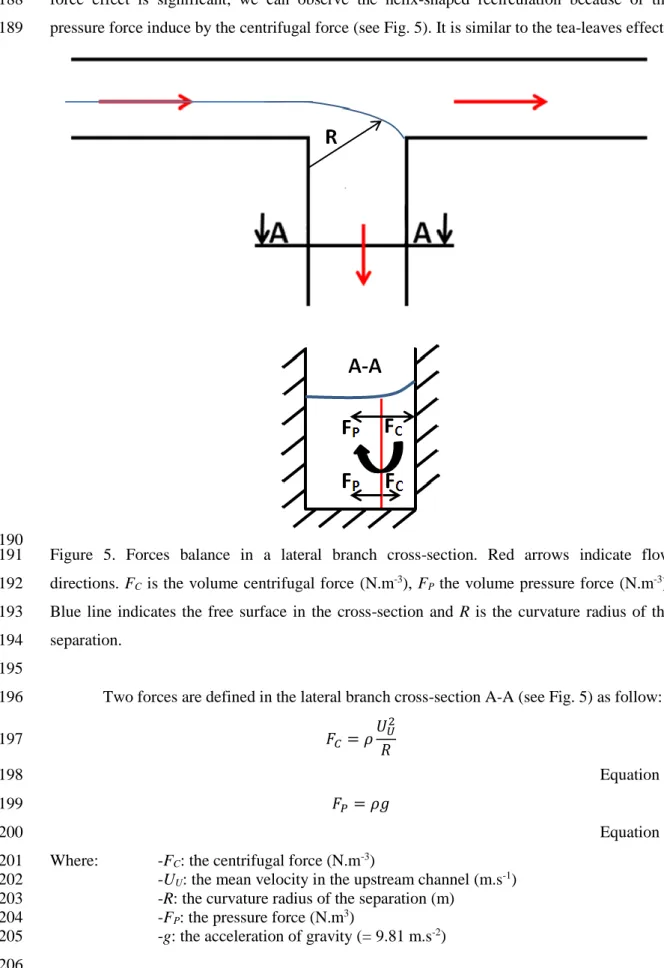
pressure force induce by the centrifugal force (see Fig. 5). It is similar to the tea-leaves effect. 189
190
Figure 5. Forces balance in a lateral branch cross-section. Red arrows indicate flow 191
directions. FC is the volume centrifugal force (N.m-3), FP the volume pressure force (N.m-3). 192
Blue line indicates the free surface in the cross-section and R is the curvature radius of the 193
separation. 194
195
Two forces are defined in the lateral branch cross-section A-A (see Fig. 5) as follow: 196 𝐹𝐶 = 𝜌 𝑈𝑈2 𝑅 197 Equation 2 198 𝐹𝑃= 𝜌𝑔 199 Equation 3 200
Where: -FC: the centrifugal force (N.m-3) 201
-UU: the mean velocity in the upstream channel (m.s-1) 202
-R: the curvature radius of the separation (m) 203
-FP: the pressure force (N.m3) 204
-g: the acceleration of gravity (= 9.81 m.s-2)
205 206
A comparison between the two defined forces gives: 207 𝐹𝐶 𝐹𝑃 =𝜌 𝑈𝑈2 𝑅 𝜌𝑔 = 𝑈𝑈2 𝑅𝑔 208 Equation 4 209
It is possible to assimilate R to the channel width B. Equation 4 becomes: 210 𝐹𝐶 𝐹𝑃 = 𝑈𝑈 2 𝐵𝑔= 𝑈𝑈2 𝐵 ℎ𝑈∙ 𝑔ℎ𝑈 = 𝐹𝑟𝑈 2 𝐵 ℎ𝑈 211 Equation 5 212
With: -hU: the water depth in the upstream channel (m) 213
Equation 5 indicates that a relationship between the squared Froude number in the 214
upstream channel FrU² and the upstream aspect ratio B/hU can determine the flow topology. 215
A numerical campaign is led to investigate this possible relationship. 216
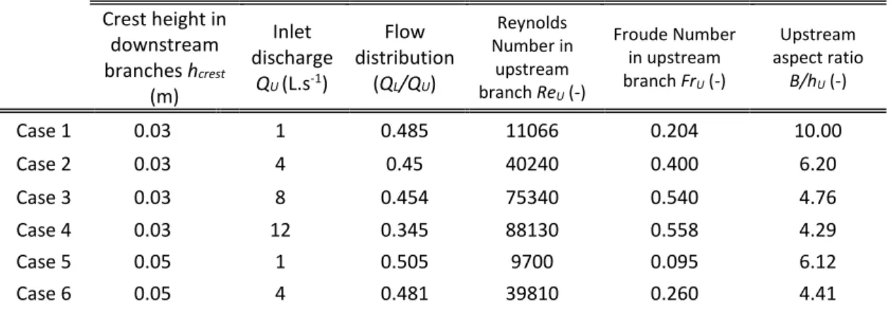
Table 4 presents the numerical campaign, comprising 16 flow cases, led to establish 217
the flow typology. For each case, Froude number is upstream channel FrU is defined as: 218 𝐹𝑟𝑈= 𝑈𝑈 √𝑔 ∙ ℎ𝑈 ∈ [0.035; 0.558] 219
Reynolds number in upstream channel ReU is defined as: 220 𝑅𝑒𝑈= 4 ∙ 𝑈𝑢∙ 𝐵 ∙ ℎ𝑈 𝜐 ∙ (𝐵 + 2 ∙ ℎ𝑈) ∈ [7400; 103900] 221
With : -UU: the mean velocity in the upstream channel (m.s-1) 222
-B: the channel width (m) 223
-hU: the upstream channel water depth (m) 224
All tested cases are thus subcritical and turbulent (see Table 4). 225
For this campaign, the crest height in both outlet branches CD and CL (CD = CL) and 226
the upstream discharge QU are the two varying boundary conditions which permit to vary the 227
two independent parameters: FrU and B/hU. 228
229
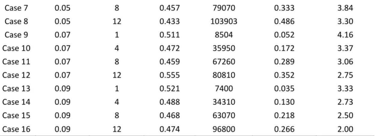
Table 4. Simulated cases for the typology numerical campaign. 230 Crest height in downstream branches hcrest (m) Inlet discharge QU (L.s-1) Flow distribution (QL/QU) Reynolds Number in upstream branch ReU (-) Froude Number in upstream branch FrU (-) Upstream aspect ratio B/hU (-) Case 1 0.03 1 0.485 11066 0.204 10.00 Case 2 0.03 4 0.45 40240 0.400 6.20 Case 3 0.03 8 0.454 75340 0.540 4.76 Case 4 0.03 12 0.345 88130 0.558 4.29 Case 5 0.05 1 0.505 9700 0.095 6.12 Case 6 0.05 4 0.481 39810 0.260 4.41
Case 7 0.05 8 0.457 79070 0.333 3.84 Case 8 0.05 12 0.433 103903 0.486 3.30 Case 9 0.07 1 0.511 8504 0.052 4.16 Case 10 0.07 4 0.472 35950 0.172 3.37 Case 11 0.07 8 0.459 67260 0.289 3.06 Case 12 0.07 12 0.555 80810 0.352 2.75 Case 13 0.09 1 0.521 7400 0.035 3.33 Case 14 0.09 4 0.488 34310 0.130 2.73 Case 15 0.09 8 0.468 63070 0.218 2.50 Case 16 0.09 12 0.474 96800 0.266 2.00 231
Fig. 6 shows the distribution of each recirculation structure, according to two parameters: 232
squared upstream Froude number FrU² and upstream aspect ratio B/hU. Both regions are 233
clearly separated from each other: a linear – at least with the present set of experiments – 234
oblique boundary separates the two types. For low FrU² and high B/hU values, the closed 235
recirculation takes place whilst for high FrU² and low B/hU values, the helix-shaped 236
recirculation occurs. 237
238
Figure 6. Flow typology in the lateral branch. Flow F1 and F2 are circled. The red-dashed line 239
represents the boundary between a classic recirculation in lateral branch and a helix-shaped 240
one. 241
5 Conclusions and perspectives 242
The present papers aimed at defining the flow patterns occurring in the lateral branch of an 243
open-channel bifurcation. A typology comprising two flow structures was established based 244
on the characteristics of the recirculation zone. The two structures are named i. “closed 245
recirculation”, similar to the flow pattern previously described in the literature and ii. “helix-246
shaped recirculation” for which the flow pattern strongly differs and is described in the 247
present paper. Both structures were observed using both experimental and numerical 248
approaches. Following the assumptions of a smooth and turbulent flow regime and equal weir 249
crest heights at both outlets, the typology is based on the comparison between centrifugal 250
force effect and pressure force effect by the mean of squared upstream Froude number FrU² 251
and upstream aspect ratio B/hU and exhibits two clear regions of recirculation structure 252
occurrence. 253
As perspectives, bed friction effect should be investigated, as well as Reynolds number effect. 254
As the define flow topology depends on curvature radius of the separation, the effect of 255
channel width ratio and discharge repartition will have an effect and should also be 256
investigated. 257
Acknowledgements 258
These works are part of the laboratory of excellence IMU (Smartness on Urban Worlds) and 259
the OTHU (Field Observatory for Urban Hydrology) at Lyon. Authors would like to thank: 260
the French ministry of research for the Ph.D. funding and the ANR (National Agency for 261
research) project funding (ANR-11-ECOTECH-007-MENTOR) and the INSU (National 262
Institute for Universe Science, project EC2CO-Cytrix 2011 project No 231). 263
Notations 264
B = channel width (m)
265
CL = crest height in the lateral branch (m) 266
CD = crest height in the downstream branch (m) 267
FC = centrifugal force (N.m-3) 268
FP = pressure force (N.m-3) 269
FrU = Froude number in upstream channel (-) 270
GCIX = grid convergence index value for variable X (dimension of variable X) 271
hU = water depth in the upstream channel (m) 272
hL = water depth in the lateral branch (m) 273
hD = water depth in the downstream branch (m) 274
hcrest = crest height for case F1 and F2 (m) 275
k = wall roughness (m)
276
NC = number of cells of the coarse mesh (-) 277
NF = number of cells of the fine mesh (-) 278
P0 = atmospheric pressure (Pa) 279
QU = upstream discharge (L.s-1) 280
QL = lateral branch discharge (L.s-1) 281
QD = downstream branch discharge (L.s-1) 282
r = cell number ratio between fine mesh and coarse mesh (-)
283
R = curvature radius of the separation zone (m)
284
ReU = Reynolds number in upstream branch (-) 285
UInlet = numerical velocity set at the inlet cross-section of the upstream channel (m.s-1) 286
UU = mean velocity in the upstream channel (m.s-1) 287
XC = value of variable X for coarse mesh (variable) 288
XF = value of variable X for fine mesh (variable) 289 z = elevation (m) 290 ν = viscosity of water (= 1.10-6 m2.s-1) 291
References
292Chu, V. H., Liu, F., & Altai, W. (2004). Friction and confinement effects on a shallow 293
recirculating flow. Journal of Environmental Engineering and Science, 3(5), 463-475. 294
Dufresne, M., Dewals, B. J., Erpicum, S., Archambeau, P., & Pirotton, M. (2010). 295
Experimental investigation of flow pattern and sediment deposition in rectangular 296
shallow reservoirs. International Journal of Sediment Research, 25(3), 258-270. 297
Grace, J. L. & Priest, M. S. (1958). Division of flow in open channel junctions. Bulletin 298
No.31. Engineering Experiment Station, Alabama Polytechnic Institute.
299
Grotjans H. & Menter F. R. 1998. Wall functions for industrial applications. In Proceedings 300
of Computational FluidDynamics’98, ECCOMAS, 1(2), Papailiou KD (ed.). Wiley: 301
Chichester, U.K.. 1112–1117 302
Hsu, C. C., Tang, C. J., Lee, W. J. & Shieh, M. Y. (2002). Subcritical 90 equal-width open-303
channel dividing flow. Journal of Hydraulic Engineering, 128(7), 716-720. 304
Kasthuri B. & Pundarikanthan N. V. (1987). Discussion of “Separation zone at open channel 305
junctions”. Journal of Hydraulic Engineering, 113(4), 543. 306
Launder B. E., Reece G. J. & Rodi W. (1975). Progress in the Development of a Reynolds-307
Stress Turbulence Closure. Journal of Fluid Mechanics. 68(3). 537–566 308
Li X. & Djilali N. (1995). On the scaling of separation bubbles. JSME international journal. 309
Series B, fluids and thermal engineering, 38(4), 541-548.Mignot, E., Zeng, C.,
310
Dominguez, G., Li, C. W., Rivière, N. & Bazin, P. H. (2013). Impact of topographic 311
obstacles on the discharge distribution in open-channel bifurcations. Journal of 312
Hydrology, 494, 10-19. 313
Mignot, E., Doppler, D., Riviere, N., Vinkovic, I., Gence, J. N. & Simoens, S. (2014). 314
Analysis of flow separation using a local frame-axis: application to the open-channel 315
bifurcation. Journal of Hydraulic Engineering. 280-290. 316
Momplot, A., Lipeme Kouyi, G., Mignot, E., Rivière, N. & Bertrand-Krajewski, J.-L. (2013) 317
URANS Approach for Open Channel Bifurcation Flows Modelling. 7th International 318
Conference on Sewer Processes and Network, Sheffield, August 2013, 8 pages.
319
Neary, V. S., Sotiropoulos, F. & Odgaard A. J. (1999). Three-dimensional numerical model 320
of lateral intake inflows. Journal of Hydraulic Engineering, 125(2), 126-140. 321
Ramamurthy, A. S., Tran, D. M. & Carballada, L. B. (1990). Dividing flow in open channels. 322
Journal of Hydraulic Engineering, 116(3), 449-455.
323
Ramamurthy, A. S., Qu, J. & Vo, D. (2007). Numerical and experimental study of dividing 324
open-channel flows. Journal of Hydraulic Engineering, 133(10), 1135-1144. 325
Rivière, N., Travin, G. & Perkins R. J. (2007). Transcritical flows in open channels junctions. 326
Proceedings, 32nd IAHR Congress, Venice, Italy, IAHR, paper SS05-11.
327
Rivière, N., G. Travin, and R. J. Perkins (2011), Subcritical open channel flows in four branch 328
intersections, Water Resour. Res., 47, W10517, doi:10.1029/2011WR010504. 329
Shettar, A. S. & Keshava Murthy, K. (1996). A numerical study of division of flow in open 330
channels. Journal of Hydraulic Research, 34(5), 651-675. 331