HAL Id: hal-01796021
https://hal-amu.archives-ouvertes.fr/hal-01796021
Submitted on 2 Jun 2018
HAL is a multi-disciplinary open access
archive for the deposit and dissemination of
sci-entific research documents, whether they are
pub-lished or not. The documents may come from
teaching and research institutions in France or
abroad, or from public or private research centers.
L’archive ouverte pluridisciplinaire HAL, est
destinée au dépôt et à la diffusion de documents
scientifiques de niveau recherche, publiés ou non,
émanant des établissements d’enseignement et de
recherche français ou étrangers, des laboratoires
publics ou privés.
Searching Data Cube for Submerging and Emerging
Cuboids
Viet Phan-Luong
To cite this version:
Viet Phan-Luong. Searching Data Cube for Submerging and Emerging Cuboids. 2017 IEEE 31st
International Conference on Advanced Information Networking and Applications (AINA), Mar 2017,
Taipei, France. �10.1109/AINA.2017.77�. �hal-01796021�
Searching Data Cube for Submerging and Emerging
Cuboids
Viet Phan-Luong Aix-Marseille Universit´e
LIF - UMR CNRS 7279 Marseille, France Email: viet.phanluong@lif.univ-mrs.fr
Abstract—Many existing approaches to data cube computation search for the group-by partitions on fact table with support greater than some threshold, that is, those can be obtained from the SQL group-by queries with the clause HAVING COUNT(*) >= supp, where supp is a support threshold. Those partitions constitute what is called the iceberg data cube.
The present work proposes an efficient method to compute the similar partitions, but in contrast to those previous approaches, in the clause HAVING, COUNT(*) can be >= supp or < supp. Generally, the method can search for the partitions that can be in the emerging part or in the submerging part of data cube, and on any other aggregate functions, not only the function COUNT. Keywords-Data warehouse, Data mining, Iceberg data cube, Infrequent itemset.
I. INTRODUCTION
The concept of data cube [1] offers important interests to business intelligence by providing aggregate views over multiple combinations of dimensions of data. These views help managers to make appropriate decision in their business. In fact, for a fact table 𝑅 with 𝑛 dimensions and 𝑘 measures, the data cube on 𝑅 can be seen as the collection of all results of the Structured Query Language (SQL) group-by queries over all subsets of the dimension scheme of𝑅, with aggregate functions on the measures. The result of each such a query is called a cuboid.
The concept is simple, but the computation and storage space of data cube can have important issues, because of the exponential number of cuboids and the big volume of the fact table in data warehouse. Iceberg data cube [2][3][4][5] is a restriction to the concept of data cube to limit the computation and the storage space: instead of computing all aggregate tuples of the cuboids, only those with COUNT value above certain thresholds are computed.
Related to research in frequent itemset mining [6], tuples in iceberg data cube are in fact frequent itemsets, as the aggregate function COUNT computes the support of tuples that represent the partition groups. Methods for mining frequent itemsets are broadly applied in association rule mining and in classification. In market basket, frequent itemsets represent the items that frequently appear in the transactions, and association rules represent the relations between the frequent itemsets. Such relations help decision on market prospecting, investment pre-vision, etc. Many efficient algorithms for mining association rules and classification based on frequent itemsets as [6], CBA
[7], CMAR [8], HARMONY [9], SIM [10]. As in data cube, all itemsets are available with their support, it is interesting to use data cube for searching for frequent itemsets and apply it to extract information as association rules, classification, page ranking, etc.
In contrast to research in frequent itemsets, research in infrequent itemsets [11] [12] searches for rare items: those that do not frequently appear. Computing infrequent itemsets are in general more cost than search for frequent itemsets. However, infrequent itemsets represent important interests in prevention of risk, intrusion, or anomalies. Related to research in data cube, tuples in cuboids with COUNT value less than the support threshold are infrequent itemsets. But iceberg data cubes exclude those itemsets.
Many other approaches to data cube search to represent the entire data cube with efficient methods for computation and storage [13][14][15]. The computing time and storage space can be optimized based on equivalence relations defined on aggregate functions [16] [17] or on the concept of closed itemsets in frequent itemset mining [18] or by reducing redundancies between tuples in cuboids, using tuple references [13][19] [16][20] [21][17][22][23]. In these approaches, the computation is usually organized on the complete lattice of subschemes of the fact table dimension scheme. The computa-tion can traverse the complete lattice in a top-down or bottom-up manner. For grobottom-uping tbottom-uples to create cuboids, the sort operation can be used to reorganize tuples: tuples are grouped over the prefix of their scheme and the aggregate functions are applied to the measures. To optimize the storage space of a cuboid, only aggregated subtuples with aggregated measures are directly stored on disk. Non-aggregated subtuples are not stored but represented by references to the (sub)tuples where the non aggregated tuples are originated or to tuples in the fact table.
Using a representation of the entire data cube, we can mine frequent or infrequent itemsets by querying data cube with the aggregate function COUNT. However, when we change the support threshold we need to renew the query, and need to re-read the entire data cube.
The work [24] proposed another approach to compute and to represent the entire data cube that is not based on the complete lattice, neither on the reduction of the storage of cuboids. By this approach, the entire data cube is represented by a half number of its cuboids. These cuboids are characterized by their
schemes: all their schemes contain the last dimension of the dimension scheme of the fact table. The other cuboids of the data cube can be obtained from the representation by a simple operation. Another difference from the above approaches is that, instead of computing the data cube for a specific aggregate function, in the approach [24], the representation is prepared for computing the data cube on any aggregate function.
A. Contributions
This work is developed on the paper [24] that presents a simple and efficient approach to represent the entire data cubes. The main ideas of [24] are:
1) Among the cuboids of a data cube, there are ones that can be easily and quickly got from the others, with no important computing time. We call these others the prime and next-prime cuboids.
2) The set of all prime and next-prime cuboids, called the last-half data cube, is computed and stored on disk using an integrated binary search prefix tree structure for compact representation and efficient search. In contrast to the other approaches, the approach in [24] does not compute the data cube representation for a specific aggregate function, neither for a specific measure. But it compute a representation that allows for computing all cuboids with any measure and any aggregate function. In fact, for each cuboid in the representation, it computes an index: each tuple in the cuboid is associated with a set of rowIds that reference to tuples in the fact table.
Based on this representation, the present work proposes an approach to mine both frequent and infrequent itemsets that allows for avoiding to re-read the entire data cube when changing the threshold and allows for mining with non-fixed threshold.
The contribution consists of the followings:
– We define the concepts of emerging and submerging tuples and cuboids that generalize the concepts of frequent and infrequent itemsets.
– An intermediate structure for cuboid storage that allows for efficient search for both emerging and submerging tuples and cuboids based on the last-half representation. Indeed, pruning technique can be done when searching frequent and infrequent itemsets on this structure.
– The implementation of these algorithms and the experi-mentation that allows to evaluate the approach.
The paper is organized as follows. Section 2 recalls the main concepts and algorithms in [24], in particular, the concept of prime and next-prime schemes and cuboids, and an algorithm for computing the group-by SQL with aggregate functions on data cube. Section 3 recalls the concepts in mining frequent and infrequent itemsets. These concepts are generalized in the concepts of emerging and submerging cuboids. It presents a structure and algorithms for efficient mining submerging and emerging cuboids. Section 4 reports the experimental results. Finally, discussion and conclusion are in Section 5.
II. LAST-HALF DATA CUBE REPRESENTATION
This section recalls the main concepts and algorithms pre-sented in [24].
A. A structure of the power set
A data cube over a dimension scheme𝑆 is the set of cuboids built over all subsets of𝑆, that is the power set of 𝑆. As in most of existing work, attributes (dimensions) are encoded in integer, let us consider 𝑆 = {1, 2, ..., 𝑛}, 𝑛 ≥ 1. The power set of𝑆 can be recursively defined as follows.
1) The power set of 𝑆0= ∅ (the empty set) is 𝑃0= {∅}. 2) For 𝑛 ≥ 1, the power set of 𝑆𝑛 = {1, 2, ..., 𝑛} can be
recursively defined as follows:
𝑃𝑛 = 𝑃𝑛−1∪ {𝑋 ∪ {𝑛} ∣ 𝑋 ∈ 𝑃𝑛−1} (1)
𝑃𝑛 is the union of 𝑃𝑛−1 (the power set of 𝑆𝑛−1) and the set in which each element is got by adding𝑛 to each element of 𝑃𝑛−1.
Let us call 𝑃𝑛−1 the first-half power set of 𝑆𝑛 and the second operand of𝑃𝑛 the last-half power set of𝑆𝑛.
Example 1: For𝑛 = 3, 𝑆3= {1, 2, 3}, we have:
𝑃0= {∅};
𝑃1= {∅, {1}};
𝑃2= {∅, {1}, {2}, {1, 2}};
𝑃3= {∅, {1}, {2}, {1, 2}, {3}, {1, 3}, {2, 3}, {1, 2, 3}}.
The first-half power set of 𝑆3 is {∅, {1}, {2}, {1, 2}} and the last-half power set of𝑆3is{{3}, {1, 3}, {2, 3}, {1, 2, 3}}.
B. Last-half data cube and first-half data cube
We call:
– A scheme in the last-half power set a prime scheme and a cuboid over a prime scheme a prime cuboid. Note that all prime schemes contain the last attribute𝑛 and any scheme that contains attribute𝑛 is a prime scheme.
– For efficient computing, the prime cuboids are computed by pairs. composed of two prime cuboids. The scheme of the first one has attribute (dimension) 1 and the scheme of the second one is obtained from the scheme of the first one by deleting attribute1. We call the second prime cuboid the
next-prime cuboid.
– The set of all cuboids over the prime (or next-prime) schemes is called the last-half data cube. The set of all remaining cuboids is called the first-half data cube. In this approach, the last-half data cube is computed and stored on disks. Cuboids in the first-half data cube are computed as queries based on the last-half data cube.
C. Integrated binary search prefix tree
For efficient storage and search in cuboids, [24] proposed to store cuboids in an integrated binary search prefix tree structure (BSPT). With this structure, tuples with the same prefix are stored as follows:
– The prefix is stored once.
– The suffixes of those tuples are organized in siblings and stored in a binary search tree.
Precisely, in C language, the structure is defined by :
typedef struct bsptree Bsptree; // Binary search prefix tree struct bsptree{ Elt data; // data at a node
Ltid *ltid; // list of RowIds Bsptree *son, *lsib, *rsib;};
where𝑠𝑜𝑛, 𝑙𝑠𝑖𝑏, and 𝑟𝑠𝑖𝑏 represent respectively the son, the left and the right siblings of nodes. With this representation, each binary search tree contains all siblings of a node in the normal prefix tree.
The field 𝑙𝑡𝑖𝑑 is reserved for the list of tuple identifiers (𝑅𝑜𝑤𝐼𝑑) associated with nodes. For efficient memory use,
𝑙𝑡𝑖𝑑 is stored only at the last node of each path in the BSPT.
Example 2:
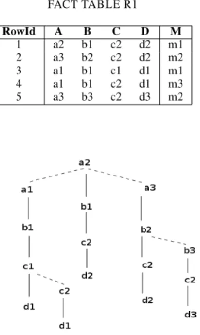
Consider Table I that represents a fact table over the dimen-sion scheme 𝐴𝐵𝐶𝐷 and a measure 𝑀. Figure 1 represents the BSPT of the tuples over the scheme 𝐴𝐵𝐶𝐷 of the fact table R1, where we suppose that with the same letter 𝑥, if
𝑖 < 𝑗 then 𝑥𝑖 < 𝑥𝑗, e.g., 𝑎1 < 𝑎2 < 𝑎3. In this figure, the
continuous lines represent the son links and the dashed lines represent the lsib or rsib links.
TABLE I FACT TABLE R1 RowId A B C D M 1 a2 b1 c2 d2 m1 2 a3 b2 c2 d2 m2 3 a1 b1 c1 d1 m1 4 a1 b1 c2 d1 m3 5 a3 b3 c2 d3 m2
Fig. 1. A binary search prefix tree
Algorithm Tuple2Ptree: Insert a tuple into a BSPT.
Input: A BSPT represented by node 𝑃 , a tuple 𝑙𝑑𝑎𝑡𝑎 and its
list of tids𝑙𝑡𝑖.
Output: The tree𝑃 updated with 𝑙𝑑𝑎𝑡𝑎 and 𝑙𝑡𝑖. Method:
If (P is null) then
create P with P->data = head(ldata), P->son = P->lsib = P->rsib = NULL; if queue(ldata) is null then P->ltid =lti;
else P->son = Tuple2Pree(P->son, queue(ldata), lti); Else if (P->data > head(ldata)) then
P->lsib=Tuple2Ptree(P->lsib, ldata,lti); else if (P->data < head(ldata)) then
P->rsib=Tuple2Ptree(P->rsib, ldata,lti); else if queue(ldata) is null then
P->ltid = append(P->ltid, lti);
else P->son = Tuple2Ptree(P->son, queue(ldata), lti); return P;
In the Tuple2Ptree algorithm,ℎ𝑒𝑎𝑑(𝑙𝑑𝑎𝑡𝑎) returns the first element of 𝑙𝑑𝑎𝑡𝑎, 𝑞𝑢𝑒𝑢𝑒(𝑙𝑑𝑎𝑡𝑎) returns the queue of 𝑙𝑑𝑎𝑡𝑎 after removing ℎ𝑒𝑎𝑑(𝑙𝑑𝑎𝑡𝑎), and 𝑎𝑝𝑝𝑒𝑛𝑑(𝑃 ->𝑙𝑡𝑖𝑑, 𝑙𝑡𝑖) adds the list𝑙𝑡𝑖 of 𝑡𝑖𝑑𝑠 to the list of tids associated with node 𝑃 .
Using the Tuple2Ptree algorithm we can create a BSPT on a table of tuples. In this BSPT, tuples are regrouped over the dimension scheme of the table, hence constitute a cuboid. As nodes corresponding to each attribute of tuples are organized in binary search tree structures, we can get the cuboid with groups of tuples in increasing (or decreasing) order.
In what follows, we consider a fact table𝑅 over a dimension scheme𝑆 = {1, 2, ..., 𝑛} and the measures 𝑀1, ..., 𝑀𝑘.
D. Computing the last-half data cube
The last-half data cube on the fact table 𝑅 can be built as follows.
– Firstly, build the prime and next-prime cuboids based on the fact table, one over𝑆 and the other over 𝑆 − {1}. To keep the computation track, the scheme𝑆 is added to a list called the running scheme and denoted by RS.
– In the following, for the currently pointed scheme 𝑋 in RS, for each dimension 𝑗 ∈ 𝑋, 𝑗 ∕= 1 and 𝑗 ∕= 𝑛 (𝑛 is the last dimension of the fact table), if𝑋 − {𝑗} is not yet in RS, then we append 𝑋 − {𝑗} to RS, and build the cuboids over
𝑋 − {𝑗} and 𝑋 − {𝑗} − {1} based on the previously built
cuboid over𝑋.
In RS, each prime scheme is associated with information that allows to locate the corresponding prime and next-prime cuboids stored on disk.
Example 3: Generation of running scheme (RS).
Table II shows the simplified last-half data cube generation process on the fact table 𝑅 over the dimension scheme
𝑆 = {1, 2, 3, 4, 5}. It shows only generation of the prime
cuboid schemes. The prime schemes appended to RS are in the first column named RS. The final state of RS is
{12345, 1345, 1245, 1235, 145, 135, 125, 15}. In Table II the
schemes marked with x (e.g., 145x) are those already added to RS and are not re-appended to RS.
E. Data Cube representation
The data cube of 𝑅 is represented by three elements: 1) The last-half data cube of which the cuboids are precom-puted and stored on disk in the format of BSPT.
2) The running scheme RS: Each prime scheme in RS has an identifier number that allows to locate the files corresponding to the prime and next-prime cuboids in the last-half data cube. 3) A relational table 𝐹 over 𝑅𝑜𝑤𝐼𝑑, 𝑀1, ..., 𝑀𝑘 that rep-resents the measures associated with each tuple of𝑅.
TABLE II
GENERATION OF THE RUNNING SCHEME OVER𝑆 = {1, 2, 3, 4, 5}.
RS Generated 12345 1345 1245 1235 1345 145 135 1245 145x 125 1235 125x 135x 145 15 135 15x 125 15x 15
Clearly, such a representation reduces about 50% space of the entire data cube, because it consists mainly of the last-half data cube stored in the BSPT format.
F. Computing the first-half data cube
Let 𝑋 = {𝑥𝑖1, ..., 𝑥𝑖𝑘} be the scheme of a cuboid in the first-half data cube that we need to retrieve (𝑋 ⊂ {1, 2, ..., 𝑛}). The size of𝑋 is 𝑘 (𝑘 < 𝑛). Based on the last-half data cube, the cuboid over 𝑋 is computed as follows.
Let𝐶 be the stored cuboid over 𝑋 ∪ {𝑛} (𝐶 is in the last-half data cube). The only difference between the scheme of
𝐶 and 𝑋 is the last attribute 𝑛. As tuples of a prime or
next-prime cuboid are stored in the BSPT format, tuples with the same prefix are regrouped together. To build the cuboid over
𝑋 based on 𝐶, we can read 𝐶 sequentially and for each group
of the tuples with the same prefix over 𝑋, we create a tuple for cuboid over𝑋, and merge the lists of rowIds associated to different suffixes (over attribute𝑛) to create the list of rowIds to associate with the created tuple. We call this process the
aggregate-projection of the cuboid 𝐶 on 𝑋. G. Querying data cubes
The general form of a group-by query on a fact table is: Select ListOfDimensions, f1(m1),..,fi(mi) From Fact_Table
Where ConditionsOnDimensions Group by ListOfDimensions
Having ConditionsOn f1(m1), ..., fi(mi); Where f1(m1), ..., fi(mi) are values of the aggregate functions f1, ..., fi on the measures m1, ..., mi. As we can see, the present approach does not compute the representation of the data cube for a specific measure, neither for a specific aggregate function, but it computes the representation that is ready for the computation on any measure and any aggregate function. In fact, each cuboid over a scheme 𝑋 in the last-half data cube is an index table for groups of tuples of the fact table (regrouped over 𝑋).
To get the cuboid over a scheme𝑋 with a specific measure
𝑚 and a specific aggregate function 𝑓, based on the
represen-tation in subsection II-E, we can process as follows.
1) If 𝑋 is prime or next-prime, then 1.1) Use RS to get the cuboid over 𝑋;
let 𝐶 be this cuboid. 2) Else, let 𝑆𝑐ℎ = 𝑋 ∪ {𝑛};
2.1) Use RS to get the cuboid over 𝑆𝑐ℎ;
2.2) Apply the aggregate-projection to get the cuboid over 𝑋; let 𝐶 be this cuboid.
3) For each tuple 𝑡 in the cuboid 𝐶,
3.1) If 𝑡 satisfies the WHERE condition, then 3.1.1) Using the table 𝐹 in the data cube representation (section II-E) and the rowIds associated with 𝑡 to get the set of values of the measure 𝑚 associated with 𝑡,
3.1.2) Compute 𝑓(𝑚) on this set of values. 3.1.3) If 𝑓(𝑚) satisfies the HAVING condition, then put 𝑡 and 𝑓(𝑚) into the response.
III. EMERGING AND SUBMERGINGCUBOIDS
In mining frequent itemsets and association rules, a dataset is a set of objects (transactions, tuples). Each object is rep-resented by an identifier and a list of valued attributes. Each valued attribute is called an item. Letℐ be the set of all items of a dataset𝒟. A subset of ℐ is called an itemset.
The support of an itemset 𝐼 with respect to a dataset 𝒟, denoted by 𝑠𝑢𝑝𝑝(𝐼), is the number of the objects in 𝒟 that have all the items of𝐼. The relative support of 𝐼 is the ratio
𝑠𝑢𝑝𝑝(𝐼)/∣𝐷∣, where ∣𝐷∣ is the cardinality of 𝐷.
The itemsets with support larger than some threshold
𝑚𝑖𝑛𝑠𝑢𝑝𝑝 are called frequent itemsets.
An association rule (AR) is an expression of the form𝑋 →
𝑌 , where 𝑋 and 𝑌 are itemsets and 𝑋 ∩ 𝑌 = ∅. A class-association rule (CAR) is an expression of the form𝑋 → 𝐶,
where 𝑋 is an itemset and 𝐶 a class label.
The above method for querying data cube can be used for searching frequent and infrequent itemsets by defining the condition on the function COUNT and the support thresholds, in the clause HAVING. In data warehouse, for OLAP, we need frequent analysis with various supports. By the above method, when we change the support thresholds, we need to do a new query. Moreover, on a fact table, the distribution of attribute values is usually not uniform, and for analysis, it is not adequate to use the same support threshold for all itemsets, and the above method does not allow non-fixed support threshold.
To generalize the concept of frequent and infrequent item-sets, we define the concepts of emerging and submerging aggregated tuples.
Definition 1. Given an aggregate function 𝑓 and the min
and max thresholds denoted respectively by 𝜃𝑚𝑖𝑛 and 𝜃𝑚𝑎𝑥 (𝜃𝑚𝑎𝑥 < 𝜃𝑚𝑖𝑛), an aggregated tuple 𝑡 is called submerging
(or emerging) if 𝑓(𝑡) ≤ 𝜃𝑚𝑎𝑥 (or 𝑓(𝑡) ≥ 𝜃𝑚𝑖𝑛, respectively). Given a cuboid𝐶, the set of all aggregated tuples in 𝐶 that are submerging (or emerging) is called a submerging cuboid (or an emerging cuboid, repectively).
A frequent (or infrequent) itemset is an aggregated tuple that is emerging (or submerging, respectively) with respect to the aggregate function COUNT. An iceberg data cube is the collection of all emerging cuboids with respect to COUNT.
In querying submerging or emerging cuboids, to avoid renewing the SQL group-by query and to use non-fixed 𝜃𝑚𝑖𝑛
and 𝜃𝑚𝑎𝑥 thresholds, we use a binary search tree structure where the search is organized on the concerned aggregate function values. As many different aggregated tuples (partition groups of a SQL group-by query) can have the same aggregate function value, each such a value is associated with a list of the representative rowIds: one rowId per partition group. Concretely, we use the following binary search tree structure.
A. Binary search tree structure on aggregate function
The binary search tree structure for querying submerging and emerging cuboids, called the binary search tree structure on aggregate function (BSTA), is defined in C language as follows.
typedef struct bsta BSTA; struct bsta { Ltid *lti;
int val; int len;
BSTA *lsib, *rsib; };
The binary tree is organized on the order of the val field. When running the group-by SQL query with COUNT function, the count value is stored in val. In general, the val field is used for the aggregate function value. All groups with the same value of val but different on attribute data (different rowIds) are stored at one node of the BSTA tree. The list of tids of these groups (one rowId per group) is stored in the lti field. The field len represents the number of groups (length of lti) that have same value on the aggregate function.
B. Building BSTA
The BSTA tree is built incrementally by inserting ag-gregated tuples into an empty tree using the algorithm
In-sert2BSTA.
Algorithm Insert2BSTA
Input: a BSTA tree B, a rowId tid, and a value val (the
aggregate function value of the group represented by row tid).
Output: The tree B updated with tid and val. Method:
if (B is NULL) {
Create B; B->lti = NULL; Insert tid into B->lti; B->val = val; B->len = 1;
B->lsib = NULL; B->rsib = NULL; }
else
if (val < B->val)
B->lsib=Insert2BSTA(B->lsib,tid,val); else if (val > B->val)
B->rsib=Insert2BSTA(B->rsib,tid,val); else {
Insert tid into B->lti; Increase (B->len); }
return B;
C. Algorithm GetAll
As the BSTA is organized on the order of the values of aggregate function, given a threshold (𝜃𝑚𝑎𝑥 or 𝜃𝑚𝑖𝑛), it is possible that all values in some of the subtrees of the BSTA do not satisfy the threshold or all values in some of the subtrees of the BSTA satisfy the threshold. In the former case, those subtrees are pruned from the search. In the latter case, we do not need to check the condition on the thresholds when traversing the tree, and just need to get all those values with their aggregated tuples into the result file. The algorithm GetAll does this task: it gets all tuples with aggregate values of a BSTA without checking the condition on thresholds.
Algorithm GetAll: From a BSTA, get all aggregated tuples
on a scheme sch using a fact table T.
Input: a BSTA B, a dimension scheme sch, a fact table T. Output: a file f of tuples on sch with their aggregate function
value obtained from B using the fact table T.
Method:
if (B is not NULL) { write T->val to f;
for each RowId in T->lti do
write_tuple(f, sch, RowId, T); getAll(f, B->lsib, sch, T);
getAll(f, B->rsib, sch, T); }
where write_tuple(f, RowId, sch, T) write to f the projection on sch of the row identified by RowId of T.
D. Computing Emerging cuboids
Algorithm QEmergCubo: To build the emerging cuboid on
a BSTA over a dimension scheme, on a min threshold and a fact table.
Input: A BSTA B, a threshold𝜃𝑚𝑖𝑛, a dimension scheme sch, and a fact table T.
Output: The file of tuples in the emerging cuboid built on B,
𝜃𝑚𝑖𝑛, sch, and T.
Method:
if (B is not NULL) { if (T->val >= 𝜃𝑚𝑖𝑛) {
for each RowId in T->lti do
write_tuple(f, sch, RowId, T); GetAll(f, sch, B->rsib); QEmergCubo(f,B->lsib,𝜃𝑚𝑖𝑛,sch,T); } else QEmergCubo(f,B->rsib,𝜃𝑚𝑖𝑛,sch,T); }
E. Computing Submerging cuboids
Algorithm QSubmergCubo: To build the submerging cuboid
on a BSTA over a dimension scheme, on a min threshold and a fact table.
Input: A BSTA B, a threshold𝜃𝑚𝑎𝑥, a dimension scheme sch, and a fact table T.
Output: The file of tuples in the submerging cuboid built on
B,𝜃𝑚𝑎𝑥, sch, and T.
Method:
if (B is not NULL) { if (T->val <= 𝜃𝑚𝑎𝑥) {
for each RowId in T->lti do
write_tuple(f, sch, RowId, T); GetAll(f, sch, B->lsib); QSubmergCub(f,B->rsib,𝜃𝑚𝑎𝑥,sch,T); } else QSubmergCubo(f,B->lsib,𝜃𝑚𝑎𝑥,sch,T); }
F. Query Submerging/Emerging cuboids
To computing the response to submerging/emerging cuboid query on an aggregate function𝑓 applied to a measure 𝑚, we can modify the algorithm given in section II-G as follows. Let
𝑋 be the scheme of the submerging/emerging cuboid that we
need to compute.
1) If 𝑋 is prime or next-prime, then 1.1) Use the running scheme RS to get the cuboid over 𝑋; let 𝐶 be this cuboid. 2) Else, let 𝑆𝑐ℎ = 𝑋 ∪ {𝑛};
2.1) Use RS to get the cuboid over 𝑆𝑐ℎ.
2.2) Apply the aggregate-projection to get the cuboid over 𝑋; let 𝐶 be this cuboid.
3) Initialize a BSTA tree B to empty. 4) For each tuple 𝑡 in the cuboid 𝐶, 4.1) Using the table 𝐹 in the data cube representation (section II-E) and the rowIds associated with 𝑡 to get the set of values of measure 𝑚 associated with 𝑡,
4.2) Compute 𝑓(𝑚) on this set of values. 4.3) Insert 𝑡 and 𝑓(𝑚) into the BSTA tree B. 5) Apply the algorithms QSubmergCubo and QEmergCubo to the BSTA tree B.
IV. EXPERIMENTAL RESULTS
The present approach is implemented in C and exper-imented on a laptop with 8 GB memory, Intel Core i5-3320 CPU @ 2.60 GHz x 4, running Ubuntu 12.04 LTS. To get some ideas about its efficiency in data cube query-ing, we recall here some experimental results in [23] as references. The experiments in [23] were run on a Pen-tium 4 (2.8 GHz) PC with 512 MB memory under Win-dows XP. The work [23] has experimented many existing and well known methods for computing and representing data cube as Partitioned-Cube (PC), Partially-Redundant-Segment-PC (PRS-PC), Partially-Redundant-Tuple-PC (PRT-PC), BottomUpCube (BUC), Bottom-Up-Base-Single-Tuple (BU-BST), and Totally-Redundant-Segment BottomUpCube (TRS-BUC). The results were reported on real and synthetic datasets. For the present work, we report only the experimental results on two real datasets CovType [25] and SEP85L [26].
By reporting the results of [23], we do not want to really compare the present approach to those methods, because we
do not have sufficient conditions to implement and to run those methods on the same system and machine. Moreover, in those methods, the data cube representation is computed for a spe-cific measure and a spespe-cific aggregate function, whereas in the present approach, the representation is prepared for computing data cube with any measure and any aggregate function. In fact, each cuboid representation in the present approach is an index table that makes references to the tuples in the fact table. Hence, we cannot compare the present approach with the approaches cited in [23] on the run time and the storage space. Apart CovType and SEP85L, the present approach is also experimented on two other real datasets that are not used in [23]. These datasets are STCO-MR2010 AL MO [27] and
OnlineRetail [28][29]. The method for mining submerging and
emerging cuboids is experimented on all these four datasets. CovType is a dataset of forest cover-types. It has 581,012 tuples on ten dimensions with cardinality as follows: Horizontal-Distance-To-Fire-Points (5,827), Horizontal-Distance-To-Roadways (5,785), Elevation (1,978), Vertical-Distance-To-Hydrology (700), Horizontal-Distance-To-Hydrology (551), Aspect (361), Hillshade-3pm (255), Hillshade-9am (207), Hillshade-Noon (185), and Slope (67).
SEP85L is a weather dataset. It has 1,015,367 tuples on nine dimensions with cardinality as follows: Station-Id (7,037), Longitude (352), Solar-Altitude (179), Latitude (152), Present-Weather (101), Day (30), Present-Weather-Change-Code (10), Hour (8), and Brightness (2).
STCO-MR2010 AL MO is a census dataset on population of Alabama through Missouri in 2010, with 640,586 tuples over ten integer and categorical attributes. After transforming categorical attributes (STATENAME and CTYNAME), the dataset is reorganized in decreasing order of cardinality of its attributes as follows: RESPOP (9,953), CTYNAME (1,049), COUNTY (189), IMPRACE (31), STATE (26), STATENAME (26), AGEGRP (7), SEX (2), ORIGIN (2), SUMLEV (1).
OnlineRetail is a data set that contains the transactions occurring between 01/12/2010 and 09/12/2011 for a UK-based and registered non-store online retail. This dataset has incom-plete data, integer and categorical attributes. After verifying, transforming categorical attributes into integer attributes, for the experiments, we retain 393,127 complete data tuples and the following ten dimensions ordered in their cardinality as follows: CustomerID (4,331), StockCode (3,610), UnitPrice (368), Quantity (298), Minute (60), Country (37), Day (31), Hour (15), Month(12), and Year (2).
Table III presents the experimental results approximately got from the graphs in [23], where “avg QRT” denotes the average query response time and “Construction time” denotes the time to construct the (condensed) data cube. Note that, [23] did not specify whether the construction time includes the time to read/write data to files.
A. On building last-half cube and querying first-half cube
Table IV reports the experimental results of this approach on CovType, SEP85L, STCO-MR2010 AL MO and OnlineRe-tail for building the last-half cube and querying first-half cube
TABLE III
EXPERIMENTAL RESULTS IN [23]
CovType
Algorithms Storage space Construction time avg QRT PC #12.5 Gb 1900 sec
PRT-PC #7.2 Gb 1400 sec
PRS-PC #2.2 Gb 1200 sec 3.5 sec
BUC #12.5 Gb 2900 sec 2 sec
BU-BST #2.3 Gb 350 sec
BU-BST+ #1.2 Gb 400 sec 1.3 sec
TRS-BUC #0.4 Gb 300 sec 0.7 sec
SEP85L
PC #5.1 Gb 1300 sec
PRT-PC #3.3 Gb 1150 sec
PRS-PC #1.4 Gb 1100 sec 1.9 sec
BUC #5.1 Gb 1600 sec 1.1 sec
BU-BST #3.6 Gb 1200 sec
BU-BST+ #2.1 Gb 1300 sec 0.98 sec
TRS-BUC #1.2 Gb 1150 sec 0.5 sec
TABLE IV
EXPERIMENTAL RESULTS OF THIS WORK ON COVTYPE, SEP85L, STCO-MR2010 AL M, AND ONLINERETAIL
CovType Storage space Run time avg QRT
Last-Half Cube 7 Gb 1018 sec
First-Half Cube 6,2 Gb 435 sec
Data Cube 13,2 Gb 1453 sec 0.43 sec
SEP85L
Last-Half Cube 2.8 Gb 444 sec
First-Half Cube 2.6 Gb 172 sec
Data Cube 5.4 Gb 616 sec 0.34 sec
STCO-MR2010 AL MO
Last-Half Cube 3.4 Gb 740 sec
First-Half Cube 3.2 Gb 209 sec
Data Cube 6.6 Gb 949 sec 0.20 sec
OnlineRetail
Last-Half Cube 3 Gb 426 sec
First-Half Cube 2.4 Gb 185 sec
Data Cube 5.4 Gb 611 sec 0.18 sec
on the last-half cube. In this table, the term “run time” means the time from the start of the program to the time the last-half (or first-half) data cube is completely constructed, including the time to read/write input/output files.
The column avg QRT in Table IV corresponds to the average run time for retrieving a cuboid based on the precomputed and stored cuboids. That is, the average query response time for SEP85L is 172s/512 = 0.34 second and for CovType 435s/1024 = 0.43 second, because the cuboids in the last-half data cube are precomputed and stored, only querying on the first-half data cube needs computing.
B. On query with aggregate functions
Based on the representation of data cube by its last-half, The group-by SQL queries with aggregate functions can be evaluated. The queries on the following aggregate functions COUNT, MAX, SUM, AVG, and VARIANCE are experi-mented on datasets CovType and SEP85L, on the last-half and on the first-half of each data cube. The queries are in the
TABLE V
TOTAL RESPONSE TIME OF AGGREGATE FUNCTION QUERY
CovType
MAX COUNT SUM AVG VAR MEAN
Last 484 467 481 552 531 503
First 352 422 444 514 497 446
Cube 836 889 925 1066 1028 949
SEP85L
MAX COUNT SUM AVG VAR MEAN
Last 196 172 195 223 225 202
First 148 154 180 204 207 179
Cube 344 326 375 427 432 381
following simple form:
Select ListOfDimensions, f(m) From Fact_Table
Group by ListOfDimensions;
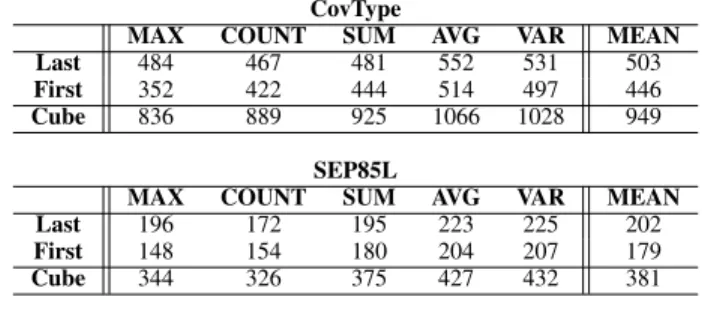
For each dataset and each half of the corresponding data cube, we compute the above query for all cuboids in the half. For instance, for the last-half data cube of CovType, we run the above query for 512 cuboids of the last-half and 512 cuboids of the first-half. In Table V, Last, First, and Cube represent respectively the last-half, the first-half data cube and the data cube itself. A value in each column of Table V represents the total query response time in seconds on the corresponding aggregate function. The total time on each line is the sum of the query response time of all cuboids of the corresponding data cube part of the line. For instance, for the last-half data cube of CovType, the total query response time is the sum of the query response time of 512 cuboids. In particular, the last column (MEAN) represents average of the total query response time on the five aggregate functions. All time includes all computing and i/o time, in particular, the time to write the results to disk.
C. On mining emerging and submerging cuboids
The approach to mine emerging and submerging cuboids is experimented on the aggregate functions COUNT and SUM using dynamic thresholds defined for each cuboid as follows:
𝜃𝑚𝑎𝑥= 𝑎𝑣𝑔(𝑣𝑎𝑙) − 𝑠𝑡𝑑𝑑𝑒𝑣(𝑣𝑎𝑙)
𝜃𝑚𝑖𝑛= 𝑎𝑣𝑔(𝑣𝑎𝑙) + 𝑠𝑡𝑑𝑑𝑒𝑣(𝑣𝑎𝑙)
where 𝑎𝑣𝑔(𝑣𝑎𝑙) and and 𝑠𝑡𝑑𝑑𝑒𝑣(𝑣𝑎𝑙) are respectively the average and the standard deviation of values (of COUNT or SUM) in the cuboid under consideration. The experiments are done on the same four datasets and for computing the submerging and emerging cuboids over all subschemes of the dimension scheme of the concerned dataset. For instance, on the dataset CovType, we compute all submerging and emerging cuboids on 1023 cuboids of the data cube. The experimental results are reported in Tables VI and VII, where – #sCub and #eCub represent respectively the number of submerging cuboids and the number of emerging cuboids.
– #stup and #etup represent respectively the average number of tuples in the submerging cuboids and the average number of tuples in the emerging cuboids.
TABLE VI
MINING SUBMERGING/EMERGING CUBOIDS ON COUNT
Dataset #sCub #stup #eCub #etup TotTime
CovType 169 574137 1023 100025 782
SEP85L 132 508387 507 153539 358
STCO-M 319 87323 1005 42052 353
OnlineR 20 79 1023 11979 278
TABLE VII
MINING SUBMERGING/EMERGING CUBOIDS ON SUM
Dataset #sCub #stup #eCub #etup TotTime
CovType 924 114416 1023 103765 1026
SEP85L 275 101883 511 63783 419
STCO-M 554 37150 1023 26515 441
OnlineR 506 58082 1023 31369 409
– TotTime represents the total time for mining all submerg-ing and emergsubmerg-ing cuboids, from the start to the end of the program, including the time to read/write data/results from/to disk. Note that the tuples are entirely write to disk, with no compact form: they are ready to be visualized.
V. DISCUSSION AND CONCLUSION
With respect to the total time for computing on CovType and SEP85L (Tables V, VI, and VII ),
– On COUNT, the total time for computing the response to all simple queries is 889s and 326s and the total time for mining all submerging and emerging cuboids is 782s and 358s. – On SUM, the total time for computing the response to all simple queries is 925s and 375s and the total time for mining all submerging and emerging cuboids is 1026s and 419s.
The computation of submerging and emerging cuboids is more complicated than retrieving simple cuboids, because we need to select only aggregated tuples that satisfy the HAVING condition. Morever, for each cuboid, we compute not only one query, but two queries: one for the emerging cuboid and the other for the submerging cuboid. However, on COUNT, the total time for mining all submerging and emerging cuboids is pretty comparable to the total time for computing the response to all simple queries. On SUM, the total time for mining both submerging and emerging cuboids is about 11% longer.
On these results, we can conclude that, based on the last-half representation of data cubes, this approach to compute submerging and emerging cuboids is efficient.
REFERENCES
[1] J. Gray et al., “Data Cube: A Relational Aggregation Operator Gen-eralizing Group-by, Cross-Tab, and Sub-Totals”, in Data Mining and Knowledge Discovery 1997 , 1 (1), pp. 29-53.
[2] Beyer, K.S., Ramakrishnan, R., “ Bottom-up computation of sparse and iceberg cubes”, in Proc. of ACM Special Interest Group on Management of Data (SIGMOD’99), 359-370.
[3] J. Han, J. Pei, G. Dong, and K. Wang, “Efficient Computation of Iceberg Cubes with Complex Measures”, in Proc. of ACM SIGMOD’01, pp. 441-448.
[4] D. Xin, J. Han, X. Li, and B. W. Wah, “Star-cubing: computing iceberg cubes by top-down and bottom-up integration”, in Proc. of VLDB’03, pp. 476-487.
[5] Z. Shao, J. Han, and D. Xin, “Mm-cubing: computing iceberg cubes by factorizing the lattice space”, in Proc. of Int. Conf. on Scientific and Statistical Database Management (SSDBM 2004), pp. 213-222. [6] R. Agrawal and R. Srikant, “Fast algorithms for mining association rules”,
in Proc. 20th Intl. Conference on Very Large Databases, VLDB’94, pp. 487-499.
[7] B. Liu and W. Hsu and Y. Ma, “Integrating Classification and Association Rule Mining“, in Proc. 4th Intl. Conference on Knowledge Discovery and Data Mining (KDD’98), pp. 80-86.
[8] W. Li and J. Han and J. Pei, “CMAR: Accurate and Efficient Classification based on multiple class-association rules“, in Proc. IEEE Intl. Conference on Data Mining (ICDM’01), 2001, pp. 369-376.
[9] J. Wang and G. Karypis, “On Mining Instance-Centric Classification Rules”, in IEEE Transactions on Knowledge and Data Engineering, Vol. 18, No.11, pp. 1497-1511.
[10] V. Phan-Luong, ”Auto Determining Parameters in Class-Association Mining”, in Proc. IEEE 26th Intl. Conference on Advanced Information Networking and Applications (AINA 2012), pp. 183-190
[11] X. Wu, C. Zhang and S. Zhang, “Efficient Mining of Both Psitive and Negative Association Rules”, in ACM Transactions on Information Systems, Vol. 22, No. 3, July 2004, pp. 381-405.
[12] L. Zhou and S. Yau, “Efficient Association Rule Mining among both fre-quent and infrefre-quent items“, in int’l journal Computers and Mathematics with Applications, 54 (2007) Elsevier, pp. 737-749.
[13] V. Harinarayan, A. Rajaraman, and J. Ullman, “Implementing data cubes efficiently”, in Proc. of SIGMOD’96, pp. 205-216.
[14] K. A. Ross and D. Srivastava, “Fast computation of sparse data cubes”, in Proc. of VLDB’97, pp. 116-125.
[15] A. Casali, S. Nedjar, R. Cicchetti, L. Lakhal, and N. Novelli, “Loss-less Reduction of Datacubes using Partitions”, in Int. Journal of Data Warehousing and Mining (IJDWM), 2009, Vol. 5, Issue 1, pp. 18-35. [16] L. Lakshmanan, J. Pei, and J. Han, “Quotient cube: How to summarize
the semantics of a data cube”, in Proc. of VLDB’02, pp. 778-789. [17] L. Lakshmanan, J. Pei, and Y. Zhao, “QC-Trees: An Efficient Summary
Structure for Semantic OLAP”, in Proc. of ACM SIGMOD’03, pp. 64-75. [18] A. Casali, R. Cicchetti, and L. Lakhal, “Extracting semantics from data cubes using cube transversals and closures”, in Proc. of Int. Conf. on Knowledge Discovery and Data Mining (KDD’03), pp. 69-78. [19] Y. Zhao, P. Deshpande, and J. F. Naughton, “An array-based algorithm
for simultaneous multidimensional aggregates”, in Proc. of ACM SIG-MOD’97, pp. 159-170.
[20] Y. Sismanis, A. Deligiannakis, N. Roussopoulos, and Y. Kotidis, “Dwarf: shrinking the petacube”, in Proc. of ACM SIGMOD’02, pp. 464-475. [21] W. Wang, H. Lu, J. Feng, and J. X. Yu, “Condensed cube: an efficient
approach to reducing data cube size”, in Proc. of Int. Conf. on Data Engineering 2002, pp. 155-165.
[22] Y. Feng, D. Agrawal, A. E. Abbadi, and A. Metwally, “Range cube: efficient cube computation by exploiting data correlation”, in Proc. of Int. Conf. on Data Engineering 2004, pp. 658-670.
[23] K. Morfonios and Y. Ioannidis, “Supporting the Data Cube Lifecycle: The Power of ROLAP”, in The VLDB Journal, 2008, Vol. 17, No. 4, pp. 729-764.
[24] V. Phan-Luong, “A Simple and Efficient Method for Computing Data Cubes”, in Proc. of 4th Int. Conf. on Communications, Computation, Networks and Technologies INNOV 2015, pp. 50-55.
[25] J. A. Blackard, “The forest covertype dataset”, ftp://ftp. ics.uci. edu/pub/machine-learning-databases/covtype, [retrieved: April, 2015]. [26] C. Hahn, S. Warren, and J. London, “Edited synoptic cloud
re-ports from ships and land stations over the globe”, http://cdiac. esd.ornl.gov/cdiac/ndps/ndp026b.html, [retrieved: April, 2015]. [27] 2010 Census Modified Race Data Summary File for Counties Alabama
through Missouri http://www.census.gov/popest/research/modified/ STCO-MR2010 AL MO.csv, [retrieved: September, 2016].
[28] Online Retail Data Set, UCI Machine Learning Repository, https://archive.ics.uci.edu/ml/datasets/Online+Retail, Source: Dr Daqing Chen, Director: Public Analytics group. chend’@’lsbu.ac.uk, School of Engineering, London South Bank University, London SE1 0AA, UK. [29] Daqing Chen, Sai Liang Sain, and Kun Guo, Data mining for the online
retail industry: A case study of RFM model-based customer segmentation using data mining, Journal of Database Marketing and Customer Strategy Management, Vol. 19, No. 3, pp. 197-208, 2012.