HAL Id: hal-01264416
https://hal.archives-ouvertes.fr/hal-01264416v2
Submitted on 2 Mar 2017
HAL is a multi-disciplinary open access archive for the deposit and dissemination of sci-entific research documents, whether they are pub-lished or not. The documents may come from teaching and research institutions in France or abroad, or from public or private research centers.
L’archive ouverte pluridisciplinaire HAL, est destinée au dépôt et à la diffusion de documents scientifiques de niveau recherche, publiés ou non, émanant des établissements d’enseignement et de recherche français ou étrangers, des laboratoires publics ou privés.
Structural Graph-Based Morphometry: a multiscale
searchlight framework based on sulcal pits
Sylvain Takerkart, Guillaume Auzias, Lucile Brun, Olivier Coulon
To cite this version:
Sylvain Takerkart, Guillaume Auzias, Lucile Brun, Olivier Coulon. Structural Graph-Based Mor-phometry: a multiscale searchlight framework based on sulcal pits. Medical Image Analysis, Elsevier, 2017, 35, pp.32-45. �10.1016/j.media.2016.04.011�. �hal-01264416v2�
Structural Graph-Based Morphometry: a multiscale
searchlight framework based on sulcal pits
Sylvain Takerkart⋆a,b, Guillaume Auziasa,c, Lucile Bruna,c, Olivier Coulona,c
⋆Corresponding author: [email protected]
a
Institut de Neurosciences de la Timone UMR 7289, Aix-Marseille Universit´e, CNRS Facult´e de M´edecine, 27 boulevard Jean Moulin, 13005 Marseille, France b
Aix-Marseille Universit´e, CNRS, Laboratoire d’Informatique Fondamentale UMR 7279 Facult´e des Sciences, 163 avenue de Luminy, Case 901, 13009 Marseille, France
c
Aix-Marseille Universit´e, CNRS, LSIS laboratory, UMR 7296
Bˆatiment Polytech Saint J´erˆome, Avenue Escadrille Normandie-Niemen, 13013 Marseille, France
Abstract
Studying the topography of the cortex has proved valuable in order to char-acterize populations of subjects. In particular, the recent interest towards the deepest parts of the cortical sulci – the so-called sulcal pits – has opened new avenues in that regard. In this paper, we introduce the first fully auto-matic brain morphometry method based on the study of the spatial organi-zation of sulcal pits – Structural Graph-Based Morphometry (SGBM). Our framework uses attributed graphs to model local patterns of sulcal pits, and further relies on three original contributions. First, a graph kernel is defined to provide a new similarity measure between pit-graphs, with few parame-ters that can be efficiently estimated from the data. Secondly, we present the first searchlight scheme dedicated to brain morphometry, yielding dense information maps covering the full cortical surface. Finally, a multi-scale inference strategy is designed to jointly analyze the searchlight information maps obtained at different spatial scales. We demonstrate the effectiveness of our framework by studying gender differences and cortical asymmetries: we show that SGBM can both localize informative regions and estimate their preferred spatial scales, while providing results which are consistent with the literature. Thanks to the modular design of our kernel and the vast array of available kernel methods, SGBM can easily be extended to include a more detailed description of the sulcal patterns and solve different statistical prob-lems. Therefore, we suggest that our SGBM framework should be useful for both reaching a better understanding of the normal brain and defining imaging biomarkers in clinical settings.
Keywords: morphometry, brain, sulcal pits, graph kernel, searchlight, multi-scale methods
1. Introduction
In the past few years, the topography of the cortical surface has raised a lot of interest, in particular to find biomarkers of pathologies (Im et al. (2012); Auzias et al. (2014)) or to detect features associated with functional specificities (Sun et al. (2012b)). In order to perform automatic morphometry based on the local organization of the cortex, studying high-level objects such as cortical sulci allows to alleviate the dependency on the one-to-one voxel/vertex correspondence which is required in traditional Voxel-Based and Surface-Based Morphometry (VBM, Ashburner and Friston (2000); SBM Van Essen et al. (2001)). This has led to the development of Object-Based Morphometry (OBM, Mangin et al. (2004)), in which each sulcus is described by a large set of attributes. OBM has been successfully used to characterize various populations of subjects, for instance by mapping gender differences Duchesnay et al. (2007) or by distinguishing patients from control subjects in pathologies such as schizophrenia Cachia et al. (2008) or autism Auzias et al. (2014).
More recently, a specific attention has been brought to the deepest part of sulci, either to elaborate theoretical models of cortical anatomy and de-velopment R´egis et al. (2005), or to automatically extract robust cortical landmarks Meng et al. (2014); Auzias et al. (2015). For the latter, the semi-nal work of Lohmann et al. (2008) has been particularly important in defining the concept of sulcal pits, with follow-ups brought by Im et al. (2010) and Auzias et al. (2015). This provides a finer spatial representation than the one offered by sulci – because a single sulcus can contain several sulcal pits. In particular, modelling local patterns of sulcal pits as graphs (see Fig.2) has proved effective in order to establish links with genetic factors Lohmann et al. (2008); Im et al. (2011) or characterize groups of patients Im et al. (2012, 2015). These studies are all based on the statistical analysis of between-subjects comparisons of pit-graphs defined within a pre-determined region of interest (ROI). These comparisons use a carefully designed similarity mea-sure described in Im et al. (2011), that relies on a spectral matching method to define pit-to-pit correspondences between subjects.
The main limitations of this ROI-based method are the following. First, the effectiveness of the similarity measure of Im et al. (2011) strongly depends
on the choice of the values of seven hyper-parameters which required a large set of specific experiments. Secondly, as with any ROI-based approach, one need to have strong a priori hypotheses to define the location and the size of the region to study. In that regard, the literature offers very little a priori information. The few published studies that looked at cortical folding patterns using sulcal pits examined either brain lobes in Im et al. (2011, 2012) or single sulcal basins Im et al. (2010); Auzias et al. (2015). Since both these approaches made it possible to detect significant effects at very different scales, it seems necessary to systematically conduct such study over a large range of spatial scales.
In order to overcome these limitations, we here introduce Structural Graph-Based Morphometry (SGBM), which is an extension of the work previously presented in Takerkart et al. (2015). This framework relies on three main contributions:
i) The design of a graph kernel that provides a new similarity measure between pit-graphs and allows – through the vast array of existing kernel methods Scholkopf and Smola (2001) – to perform various statistical analyses directly in graph space. This kernel has very few parameters that can be efficiently inferred from the data.
ii) The definition of a searchlight scheme – the first designed to perform brain morphometry – that yields information maps estimated from patterns of sulcal pits constructed at different spatial scales. Searchlight methods, introduced by Kriegeskorte et al. (2006), consist in fitting a multivariate statistical model (e.g a classifier) on patterns defined in a local neighborhood, and repeating this operation in a sliding window fashion to fully cover the brain. A summary statistic (for instance the accuracy of the classifier) is then assigned to the center of each neighborhood, thus yielding a spatial information map that allows the localization of the informative regions.
iii) The construction of a non parametric multi-scale inference strategy that facilitates this localization by jointly analyzing the searchlight informa-tion maps obtained at all scales and offers a high detecinforma-tion power. Multi-scale methods aim at studying phenomena for which the optimal scale to be used is unknown Koenderink (1984); Lindeberg (1994), as when studying the local organization of sulcal pits. They have been used in neuroimaging for various tasks, such as the description of activation patterns in PET (Coulon et al. (2000)) and fMRI (Operto et al. (2012)) data or the segmentation of sub-cortical regions in anatomical MRI (Wu et al. (2015)). Etzel et al. (2013) also suggested that multi-scale strategies could be useful to desambiguate the
a posteriori interpretation of regions detected by searchlight-based methods, which we implement here.
SGBM combines these three novelties in order to build a new fully auto-matic brain morphometry framework. This framework studies local patterns of sulcal pits by comparing them using our graph kernel, in order to define a classification-based searchlight scheme that overcomes the limitations of ROI-based approaches while embedding a multi-scale inference framework. This makes it possible to detect differences in local folding patterns at dif-ferent scales between several groups of individuals. In the following, we first present the SGBM framework step by step, including a detailed description of our three contributions. We then demonstrate the power of our frame-work on two classical brain mapping problems for which complex patterns of anatomical differences have previously been reported in the literature: the mapping of asymmetries between the left and right brain hemispheres and the detection of cortical shape differences between male and female subjects.
2. Methods
2.1. Extracting sulcal pits from T1 MR images
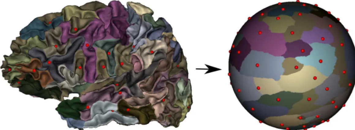
In order to obtain the sulcal pits from an anatomical MR image, we first perform the segmentation of the cortical ribbon and the cortical reconstruc-tion according to Dale et al. (1999) using the freesurfer image analysis suite 1. Then, we use the method describe in Auzias et al. (2015) to extract the sulcal pits from the cortical sheet of each subject and the Depth Potential Function of Boucher et al. (2009) to define a depth feature for each sulcal pit. This pit extraction method was carefully designed to obtain reproducible sulcal pits in every cortical region and not only in the deepest sulci, which is of critical importance to study patterns of pits centered around all cor-tical locations, as aimed at by the framework introduced in this paper. In order to compare pits between different subjects of the population S to be studied, we need to bring them into a common space. We use the cortical registration algorithm available in freesurfer Fischl et al. (1999) in order to align the convexity information across individuals after having inflated these meshes to a sphere. This sphere, onto which all subjects are aligned, will serve as our common space onto which we project the sulcal pits and basins
1www.freesurfer-software.org
of every subject, as illustrated on Fig. 1. For each subject s ∈ S, we thus obtain the set of sulcal pits Ps = {πs
i}i=N
s
i=1 localized on the sphere and their corresponding basins {βis}i=N
s
i=1 . Note that the number of pits Ns can vary across subjects.
Figure 1: Left: sulcal pits of one subject, represented on the cortical sheet. Right: after cortical registration to the template and projection to the common spherical space, in which inter-subject pits locations are compared.
2.2. Representing folding patterns as pit-graphs
A natural way to formally represent the local folding pattern of a given part of the cortex is to construct a region adjacency graph from the set of sul-cal pits and basins located within this region, as proposed in Im et al. (2011). Given a subset P ⊂ Ps of N pits (N ≤ Ns), each pit πs
i ∈ P defines a node of the graph. The graph edges are then given by the spatial adjacency of their associated basins: this defines a binary adjacency matrix A = (aij) ∈ RN ×N (aij = 1 if βi and βj are adjacent, and 0 otherwise), that encodes the spa-tial organization of the folding pattern. We can then add attributes to each graph node in order to better characterize the folding pattern. In the present paper, we use two attributes for each pit: i) its euclidean coordinates on the common sphere Xi, to compare graph nodes localization across subjects, and ii) its depth di, because it is an intrinsic characteristic of the pit. The map-ping from each subject to the common sphere explicitly minimizing metric distorsions Fischl et al. (1999), this sphere is a good space to compare pits locations across subjects in a spatially uniform manner. Note that other at-tributes can be added in the same manner without affecting the rest of the
method, making these graphs a versatile representation. Let D = {di} ∈ RN be the vector of depth values and X = {Xi} ∈ RN ×3 be the matrix of coor-dinates of all graph nodes. Any pattern of sulcal pits can therefore be fully represented by an attributed graph defined as G = (P, A, D, X ). Examples of sulcal pit graphs are shown on Fig. 2.
Figure 2: Sulcal pit-graphs in the right frontal lobe for four subjects, displayed on the inflated cortex. The node color encodes the depth of the pit, from blue (shallow) to red (deep).
2.3. Measuring pattern similarity using a graph kernel
Our first contribution is to introduce a graph kernel that provides a new similarity measure between pit-graphs. It is adapted from of a graph kernel that we designed to handle inter-subject variability in fMRI data Takerkart et al. (2014). In order to compare two pit-graphs G = (PG,AG,DG,XG) and H = (PH,AH,DH,XH), our kernel exploits the different characteristics of the graphs by comparing all pairs of nodes (i.e potential edges) gij and hkl, respectively in G and H. As such, it belongs to the class of walk-based graph kernels G¨artner et al. (2003) and uses the most elementary walks, of length one. It combines (see eq. 4) the different features of the graphs by using several sub-kernels within the convolution kernel framework Haussler (1999). A first sub-kernel acts on the graph structure itself, by ensuring that the comparisons are performed only if gij and hkl are actual edges. This is done with the linear kernel on the binary entries of the adjacency matrices:
ka(gij, hkl) = aGij.aHkl, (1)
which takes the value 1 if aG
ij = aHkl = 1 and 0 otherwise. A second sub-kernel uses a product of Gaussian kernels on the coordinates of the nodes of gij and hkl to compare the locations of edges across subjects:
kx(gij, hkl) = e−kX
G
i −XkHk2/2σ2x· e−kXjG−XlHk2/2σ2x. (2)
In practice, kx acts as a spatial filter that weights the comparisons of edges with their proximity, thus eliminating the comparisons of edges that are far away from eachother while tolerating inter-subject variability (if edges are close, but not perfectly matched across subjects). Finally, the last sub-kernel compares the depth attributes using the same principle:
kd(gij, hkl) = e−kdGi −dHkk2/2σd2· e−kd G j−d
H
l k2/2σ2d (3)
Other optional attributes that could be added to further characterize the sulcal pits would be treated in the same manner.
The full kernel is defined as the combination of all sub-kernels applied on all pairs of nodes of G and H, which gives in our case:
K(G, H) = NG X i,j=1 NH X k,l=1
ka(gij, hkl) · kx(gij, hkl) · kd(gij, hkl) (4)
Note that the number of nodes NG and NH in G and H can be different. We then perform the following normalization
˜
K(G, H) = K(G, H)
pK(G, G)K(H, H), (5) which ensures that ∀G, ˜K(G, G) = 1, i.e that the similarity between a graph and itself does not depend on the graph.
Note that this kernel has two hyper-parameters σx and σd, which are the bandwidths of the gaussian sub-kernels that respectively act on the co-ordinates and the depth features. In order to choose the values of these parameters, we use an extension of a standard practice whose effectiveness has been demonstrated in Takerkart et al. (2014): we set σx and σd to the median euclidean distances between the coordinates and depth attributes of the nodes in all graphs available at training time. Note that in the case where the pit-graphs represent local folding patterns, as in the rest of the paper, the value of σx will adapt to this property of the graphs and consequently, kx will act as a spatial filter within the neighborhood of interest.
Figure 3: Illustrations of the pit-based searchlight scheme used in our SGBM framework. A: The sulcal pits and basins of a set of subjects projected onto the common spherical space. B: The Fibonacci point set used to sample the sphere. C: Around one of these points (larger green ball), the local pit-graphs defined for each subject within a spherical neiborhood (the node color encodes the depth of the sulcal pit). D: Classifying local pit-graphs into two categories (ex: patients vs. controls). E: Repeating this at all locations to obtain the searchlight information map: the Fibonacci points are projected onto the folded (left) or inflated (right) mesh (the sphere color encodes the amount of information available at this location for the classification task).
2.4. Searchlight mapping
Our second contribution is the definition of a searchlight method (Kriegesko-rte et al. (2006)) that enables the mapping of cortical shape differences based on local folding patterns represented as sulcal pit-graphs. In order to con-struct a searchlight scheme for a given task, one needs to define the five following items: A: the domain of interest; B: the sampling strategy used to cover this domain; C: how to define local patterns at each location; D: the multivariate statistical model that addresses the task itself and E: the sum-mary statisticto be used to create the information map. We now instantiate these five items, as illustrated on Fig.3.
In order to define our pit-based searchlight scheme in a domain where the sulcal pits of all subjects can be compared, we use the common spherical
space where all subjects have been aligned (see 2.1) as our domain of inter-est (item A). Then, the Fibonacci point set (Niederreiter and Sloan (1994)) provides a pseudo-evenly distributed sampling of the sphere, with an arbi-trary number of points Q; this defines the sampling strategy of our searchlight scheme (item B). For a given location q ∈ {1, · · · , Q} and a given subject s ∈ S, we then define the set Pq,rs of sulcal pits located within a radius r of point q, i.e Ps
q,r = {πis ∈ Ps | dist(q, πis) < r}, where dist designates the euclidean distance between two points. Given this set of pits, we can directly apply the graph construction scheme described in 2.2 to obtain the attributed graph that we note Gs
q,r. The set of graphs {Gsq,r}s∈S defines the local patternsat location q (item C) that will serve as inputs to the statistical model defined hereafter.
Equipped with our graph kernel ˜K defined in 2.3, we can use any kernel method to address a wide range of problems including regression, clustering or classification. Here, we focus on supervised classification to perform group discrimination and we use a non linear Support Vector Classifier as our mul-tivariate statistical model (item D). Such a classifier is easy to estimate by using ˜K, which is a positive definiete kernel, and the so-called kernel trick – an idea that was introduced in Aizerman et al. (1964). We then assess the generalization power of the classifier by measuring its accuracy. In practice, for a given location q and a given value of r, we have a fully labeled dataset {(Gs
q,r, ys)}s=Ss=1 at our disposal, where the label ys encodes the group subject s belongs to (for instance, ys = −1 for a control subject and ys = +1 for a patient). In order to obtain the accuracy ¯ar
q of the classifier, we resort to a 10-fold cross-validation which offers a good estimate of the true accuracy Kohavi (1995).
The final step in setting up a searchlight scheme consists in defining a summary statistic from the output of the statistical model in order to con-struct the searchlight information map. Because the distribution of ¯arq is unknown, we first resort to a permutation scheme in order to estimate it under the null hypothesis of no differences between groups, as advocated in neuroimaging in general by Bullmore et al. (1999); Nichols and Holmes (2002) and more particularly in statistical analyses of searchlight information maps by Kriegeskorte et al. (2006); Stelzer et al. (2013). Assuming the stationar-ity of this null distribution over the cortex, we pool together the classifier results at all searchlight locations to obtain an estimate of the cortex-wise distribution of ¯arq. This provides a map of uncorrected point-wise p-values {pr
corresponds to pr
q, which we note zqr; this non linear transformation is in fact given by the so-called Inverse Error Function erf−1, also called Nor-mal Inverse Cumulative Distribution function. We use this zrq-score as our summary statistic (item E in the definition of our searchlight scheme), which defines the searchlight information map Zr = {zr
q}q∈[1,··· ,Q]. This Zr map can easily be used to perform inference because we estimated its underlying distribution, and presents the nice property of being highly contrasted – as compared with the original accuracy map – thanks to the non linear trans-formation used to create the zr
q-scores. The latter property will be useful at a later stage in our SGBM framework. The estimation of these information maps is implemented by the following algorithm, in which card designates the function that returns the size of the set given in input.
Algorithm 1: Computing the searchlight information map at scale r Input : a labeled dataset {(Xs, ys)}s=Ss=1
Input : a set of M permutations {Γj}j=Mj=1 , Γ1 being the identity foreach permutation Γj do
foreach searchlight location q do compute ¯ar
q(j) from the re-labeled dataset {(Gsq,r, yΓj(s))}
s=S s=1 foreach permutation Γj do
foreach searchlight location q do prq(j) = Q×M1 card({(j′, q′) | ¯ar
q′(j′) ≥ ¯arq(j))}
zrq(j) = erf−1(pr q(j))
this defines the map Zr(j) = {zr
q(j)}q∈[1,··· ,Q] Output: a set of M maps {Zr(j)}j=M
j=1
Output: the map corresponding to the true labels is Zr = Zr(1)
Note that we also compute the set of information maps {Zr(j)}j=M j=1 ob-tained for all permutations because they will be used in the following. Also, by convention, the first permutation is set to be the identity, which means that the true information map Zr is included in this set as Zr(1).
2.5. Multi-scale spatial inference
In this section, we describe our third contribution, which is a multi-scale spatial inference strategy that both localizes the regions of the cortex where folding patterns are significantly different and estimates the spatial scale of these effects. First, we repeat the previously described searchlight procedure
for a given set of ρ scales R= {r1. ,· · · , rρ}, yielding a set of information maps {Zr}
r∈R, which each comes with its permuted versions {Zr(j)}j=Mj=1 , forming a full set of M × ρ maps. Detecting at which locations q and scales r the classifier performance is above chance level – i.e testing zr
q > 0, ∀(q, r) – is a massively univariate inference problem for which it is crucial to correct for multiple comparisons. Because these information maps exhibit correlations across both scales and space, an appealing way to deal with the multiple comparisons problem is to resort to cluster-based statistics, as introduced in Poline and Mazoyer (1993) and vastly used since in the neuroimaging literature. Following the non-parametric scheme described in Bullmore et al. (1999), this can be done in three steps:
❼ applying an arbitrary threshold to a statistical map to form contiguous regions of supra-threshold locations, classically referred to as clusters; ❼ defining a cluster-wise statistic and computing it for each cluster; ❼ estimating the null distribution of the maximum cluster statistic using
a set of maps obtained by permuting the labels of the observations, which provides corrected cluster-wise p-values (see Nichols and Holmes (2002)).
Thanks to the way our zr
q statistic was designed (see 2.4), the initial cluster-forming operation is easy to perform by setting a threshold τ that corresponds to the desired one-sided uncorrected point-wise p-value; for in-stance, thresholding at zr
q > τ with τ = 3.090 corresponds to prq < 0.001. Note that because this is true for all values of r, a single threshold value can be used for all scales. Then, we need to select a cluster-wise statistic. The most commonly used one is the cluster size – the number of locations inside a cluster Poline and Mazoyer (1993), but it naturally favors large clusters. In order to avoid this bias, we use the cluster mass (Bullmore et al. (1999); Zhang et al. (2009)), i.e the sum of supra-threshold point-wise statistics, which should better preserve the chances of small clusters to be detected thanks to the high contrast of our Zr maps. Note that this potential benefit brought by using the cluster mass – instead of the cluster size – would have been lesser if we had directly used the accuracy as our summary statistic. Finally, we introduce two complementary strategies to estimate the empirical distribution of the cluster-wise statistic in this multi-scale setting. They are described in the following and summarized on Fig.4.
Figure 4: Illustrations of the two inference strategies. A: the set of permutations of the labels (each column is a permutation, black corresponds to y = −1 and white to y = +1; the first permutation in the left-most column contains the true labels). B: single-scale searchlight information maps, for each scale and each permutation. C & D: single scale clusters, and the null distributions of their maximum cluster mass, estimated from the set of permuted single-scale clusters at each scale. E, F & G: multi-scale information maps, multi-scale clusters, and the null distribution of their maximum cluster mass. The distribution shown in D and G are then used to assess the corrected p-values, respectively for the single-scale and the multi-scale clusters obtained with the true labels.
2.5.1. Single-scale clusters with corrections for multiple comparisons across space and scales
The first strategy consists in defining clusters by independently thresh-olding each Zr map. We therefore designate these as single-scale clusters in the rest of the paper. The multi-scale nature of this first inference method hails from the correction for multiple comparisons, which is performed in two steps. First, we estimate the null distributions of the maximum cluster mass separately for each single scale, by pooling the masses of clusters obtained with all permutations at the considered scale (see Alg. 2). This yields p-values corrected for the multiple comparisons due to the repetition of tests in space. Note that it was necessary to distinguish null distributions between scales because they ended up being fairly different. In a second step, we used a Bonferroni correction to account for the repetition of tests across scales: multiplying the p-values obtained in the first step by the number of scales included in the analysis allows estimating corrected p-values that take into account the repetition of tests both in space and across scales, which can then be thresholded at the desired significance level to perform inference.
Algorithm 2: Computing spatially-corrected p-values for single-scale clusters
Input : a scale r
Input : a set of permuted single-scale maps {{Zr(j)}j=M
j=1 , with the one obtained with the true labels for j = 1
Input : a threshold τ foreach permutation j do
apply thresholding on Zr(j) with zr
q(j) > τ get the set of clusters {cji}i=Nj
i=1 from the thresholded map foreach cluster cji do
compute cluster mass mji = P q∈cji
zqr(j)
compute maximum mass Mj = max i ({m
j i}i=N
j
i=1 ) foreach true cluster ci = c1i do
compute cluster mass mi = P q∈ci
zrq(1)
compute corrected p-value pi = M1 card({j | Mj ≥ mi}) Output: single-scale clusters with their p-values {ci, pi}i=N1
i=1 (corrected for multiple spatial testing)
2.5.2. Multi-scale clusters with corrections for multiple comparisons across space
Our second strategy starts by designing a statistic that summarizes the results obtained across all scales at a given location q. Because we expect an effect to be observable across several consecutive scales, we first compute a sliding average of zr
q across scales. Then, in order to detect effects potentially present at any scale, we select the maximum value from the results of the sliding average operation. This gives
ZRq = max r∈R( 1 R X r′, |r−r′|≤R/2 zqr′), (6)
where R represents the size of the averaging window used across scales. This results in a single multi-scale information map ZR = {ZR
q}q∈[1,··· ,Q], which summarizes the content of all single-scale maps {Zr}r∈R. We note {ZR(j)}j=M
j=1 the set of corresponding permuted multi-scale maps. In the following, we will use the term multi-scale clusters to designate the clusters obtained by thresholding these multi-scale information maps. By changing the second input of Alg. 2 to this {ZR(j)}j=M
j=1 set of permuted multi-scale maps, we can estimate the p-value – corrected for the repetition of tests per-formed in space – for each multi-scale cluster. Furthermore, at any location q within a significant cluster, we can estimate the preferred scale of the effect as the value of r that maximised the sliding average of zr
q across scales for the true labels:
ˆ rR(q) = arg max r∈R( 1 R X r′, |r−r′|≤R/2 zqr′) (7)
3. Experiments and results
3.1. Mapping gender and hemispheric differences
In order to explore the capabilities of our framework, we study two clas-sical brain morphometry problems: the mapping of gender differences and cortical asymmetries. Because some neurological disorders are expressed dif-ferently in males and females (see Ruigrok et al. (2014)) and others are associated with abnormal cortical lateralization Toga and Thompson (2003), studying these problems can directly provide information on the pathologies
themselves. While they have already been studied using automatic morphom-etry methods such as VBM, SBM and OBM (see 3.3), our SGBM framework should shed a new light on both questions by examining differences in the organization of local folding patterns.
For this purpose, we use data from the Open Access Series of Imag-ing Studies2 (OASIS) cross-sectional database, which offers a collection of 416 subjects aged from 18 to 96. For each subject, three to four individ-ual T1-weighted MP-RAGE scans were obtained on a 1.5T Vision system (Siemens, Erlangen, Germany) with the following protocol: in-plane resolu-tion = 256x256 (1 mm x 1 mm), slice thickness = 1.25 mm, TR = 9.7 ms, TE = 4 ms, flip angle = 10➦, TI = 20 ms, TD = 200 ms. Images were co-registered and averaged to create a single image with a high contrast-to-noise ratio. From this database, we selected two groups of 67 male and 67 female healthy right-handed subjects, aged 18 to 34.
In practice, for the gender problem, we used the 134 subjects to set up a binary classification problem, with labels defined by y = −1 for a male subject and y = +1 for a female. For the asymmetry problem, an extra pre-processing step was carried out using the symmetric cortical template described in Greve et al. (2013), as used in Auzias et al. (2015) to study pit-based asymmetries. We then used the 134 symmetrized hemispheres of the male subjects to set up a binary classifcation problem where labels are y = −1 for a left hemisphere and y = +1 for a right hemisphere. For both problems, we use a Fibonacci point set of size Q = 2500, which provides a dense enough sampling of the sphere (see Fig. 3) to observe the expected continuity in the information maps estimated by the searchlight scheme (see results hereafter). The number of permutations was set to M = 5000, en-suring that the empirical distributions are accurately estimated. The cross-validation used to estimate the average classification accuracy was carefully designed to ensure class balance in both the training and test datasets for each fold. As with any cluster-based analyses – which represent the vast ma-jority of spatial inference methods used in neuroimaging, the initial cluster-forming thresholding has an influence on the final results. With this in mind, we repeated our analysis with different threshold values and empir-ically selected the one that gave results which offered a good compromise between sensitivity and specificity. The results shown hereafter have been
obtained with a cluster-forming threshold of τ = 3.090, which corresponds to a thresholding at p < 0.001 on the uncorrected point-wise p-values as-sociated with the classification score. Finally, we used the following set of scales in order to study the multi-scale properties of local sulcal patterns: R = {30, 35, 40, 45, 50, 55, 60, 65, 70, 75, 80, 85, 90mm}. Each scale value de-. fines the radius of a searchlight spherical neighborhood that is computed on the freesurfer sphere, i.e. the common space for all subjects, which has a 100mm radius. The smallest neighborhood (30mm Euclidean radius) is a spherical cap whose surface area is 2.25% of the sphere surface area. Equiva-lently, the largest neighborhood (90mm scale) represents 20.75% of the sphere area. In other words, we use a scale range that varies between 2.25% and 20.75% of an hemisphere surface area. This will yield patterns between the size of a small gyrus and one of a brain lobe, thus covering the smallest (Im et al., 2010; Auzias et al., 2015) and largest (Im et al., 2011, 2012) effects previously reported in the literature when studying sulcal pits.
3.2. Results: methodological considerations
In this section, all the maps presented follow the same format. Each of the elements of the spherical Fibonacci point set is represented by a small sphere and projected onto the inflated cortical mesh. This allows for an easy visualization of the global maps.
3.2.1. Examining raw information maps
In order to assess the results provided by our SGBM framework, we first qualitatively observe raw single-scale and multi-scale information maps ob-tained with our pit-based searchlight scheme.
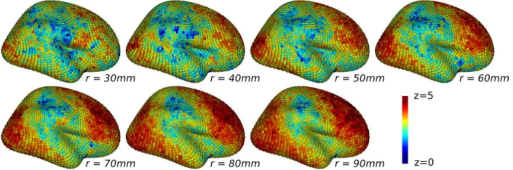
Single-scale maps Zr are shown on Fig. 5. They display some contrast at all scales r, i.e they contain locations of low and high zr
q-values, sometimes reaching zr
q = 5 or more – which corresponds to very significant uncorrected point-wise p-values (pr
q < 10−6). We can clearly observe the spatial corre-lation through the fact that the points of high statistic values are grouped together. Furthermore, the spatial smoothness of the maps and the size of the groups of searchlight locations with high zr
q-values increase with r, which is a typical behavior of searchlight information maps Kriegeskorte et al. (2006). Finally, the persistence of the regions with high zr
q-values across several con-secutive values of r attests of the correlation across scales of the Zr maps, which also supports the relevance of the construction scheme used to define the multi-scale statistic ZR
q (see Eq. 6). 16
Figure 5: Examples of raw single-scale information maps Zr
for different neighborhood radiuses r (gender differences, external face of the right hemisphere).
We now examine the multi-scale maps ZR, displayed on Fig. 6. Each of them summarizes the information contained at all scales r ∈ R. For R = 1, ZRq is the max of all zrq across all scales r; for R = card(R), i.e for R = 13 in our experiments, ZR
q is the average of zqr across all scales. Overall, these maps are smoother than the single-scale Zr maps, which is expected because the construction of the multi-scale statistic ZRq acts as a smoothing operation across scales. For the smaller values of R, the contrast of the statistic map is weaker than the one offered by single-scale maps: some very large portions of the cortex show high values of ZRq, which means that the specificity offered by low values of R is limited. For very large values of R, the maps contain less locations with high statistical values, which is also expected because in this case, a high ZRq-value reflects a phenomena that exist over a larger number of consecutive scales. Therefore, it seems adequate to use an intermediary value of R, for which ZR
q averages zqr over a limited number of consecutive scales.
3.2.2. Qualitative assessment of single-scale clusters
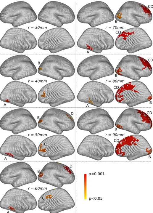
We then examine the single-scale clusters. Figs. 7 and 8 show the clusters which present a p-value lower than 0.05, after correction for multiple com-parisons across space and scales with the method described in Section 2.5.1. For both the gender and asymmetry problems, our framework detects signif-icant clusters at all scales with r at least 40mm, demonstrating its detection power. Almost all clusters are persistent across scales, i.e for a given clus-ter at scale r, there exist clusclus-ters at nearby cortical locations for nearby scales. The clusters detected at finer scales are overall smaller than the ones
Figure 6: Examples of raw multi-scale information maps ZR
(gender differences, external face of the right hemisphere). Each of these maps summarizes the information from all single-scale Zr
maps shown on Fig 5. This multi-scale statistic depends on the number R of consecutive scales r over which the single-scale statistic is averaged (see Eq. 6).
detected with larger window sizes. This is caused by the larger smoothing effect of the large window sizes (as previously observed on the raw maps, see on Fig. 5); furthermore, we noted that the critical cluster mass correspond-ing to a corrected p-value of 0.05 (estimated by the procedure described in Section 2.5.1) increases with the size of the window, which therefore discards the smallest clusters at large scales. However, some small clusters remain significant at large scales. This overall demonstrates that our cluster-based spatial inference strategy is effective; in particular, the use of the cluster mass associated with our zr
q statistic makes it possible to detect clusters at fine spatial scale and small clusters at larger scales, which is known to be challenging in practice in such a multi-scale context.
3.2.3. Qualitative assessment of multi-scale clusters
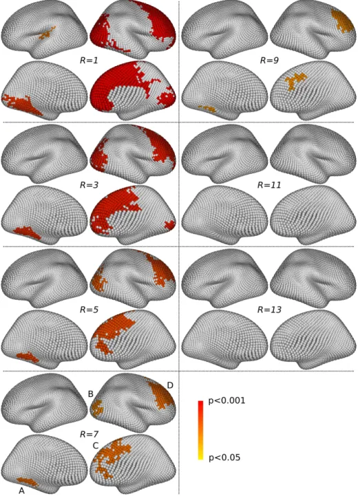
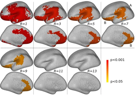
Figs. 9 and 10 show the significant clusters (corrected p < 0.05) obtained with the method described in 2.5.2, for R ∈ {1, 3, 5, 7, 9, 11, 13}. The ob-servations made previously on the raw statistic map gets confirmed: some overly large clusters are detected for the smaller values of R, while nothing is detected for larger values (R ≥ 11). This confirms that an intermediary value of R might offer a satisfactory compromise between specificity and sen-sitivity. This is concordant with the intuition that an effect can live across several consecutive scales, but not over a very large number of consecutive scales as sought after with large R values.
3.2.4. Comparing single-scale and multi-scale results
We will now compare the clusters detected by our single-scale and multi-scale approaches. Our objective is two-fold: i) to assess the consistency, or lack thereof, of the results of the two approaches, and ii) to facilitate the
Figure 7: Gender differences. For each value of r, four views are shown, two per hemi-sphere: the left hemisphere is shown on the left, and the right on the right, with re-spectively their external and internal faces at the top and the bottom. The significant single-scale clusters (corrected p < 0.05) are colored with their p-value. Four main clus-ters, tagged A, B, C and D, appear to be persistent across scales, sometimes after having
Figure 8: Asymmetries. For each value of r, the single-scale clusters presenting significant differences between the left and right hemispheres (corrected p < 0.05) are shown on the external and internal faces of the left hemisphere. Two main clusters, tagged A and B, appear to be persistent across scales.
Figure 9: Gender differences. Simlarly to Fig.7, four views are presented for each value of R, showing thresholded significant multi-scale clusters (corrected p < 0.05). For R = 7, four clusters survive, at similar locations as single-scale ones; they are tagged A, B, C and D, accordingly to Fig. 7.
Figure 10: Asymmetries. Significant muli-scale thresholded clusters. For R = 7, the same two clusters as in the single-scale analysis are detected; they are tagged A and B, accordingly to Fig. 8.
selection of the value of the R parameter of our multi-scale statistic.
For the gender problem, we examine Fig. 7 (single-scale clusters) and Fig. 9 (multi-scale clusters). The single-scale approach detects clusters in four main locations (tagged A, B, C and D on Fig. 7), which are present across a large number of scales. Their precise location and extent vary smoothly across scales. For instance, the cluster at location B slightly moves forward when the scale r increases; some merging phenomena also happen between clusters, as with the clusters at locations C and D, which are separated at scales r ≤ 60mm and fused into one larger cluster at scales r ≥ 70mm. The multi-scale approach detects clusters in similar locations for various values of the R parameter; however, the results with R = 7 are the only ones for which there are four separated clusters at the four locations A, B, C and D. For the asymmetry problem, we examine Fig. 8 (single-scale clusters) and Fig. 10 (multi-scale clusters). The single-scale approach detects clusters in two main locations (tagged A and B on Fig. 8), which are present across almost the full range of scales from r = 30mm to r = 90mm. The clusters present around these locations also fuse together for r ≥ 80mm. The multi-scale approach detects clusters in similar locations for various values of the R parameter; however, only the results obtained with R = 7 and R = 9 provide two separated clusters for each location A and B.
Overall, both our single- and multi-scale inference strategies offer satis-factory detection power. The fact that the significant clusters of both ap-proaches occupy similar locations clearly demonstrates their consistency. In order to choose the value of the parameter R of the multi-scale strategy, we showed that choosing an intermediary value provides a good compromise be-tween sensitivity and specificity, as found in our restults with R = 7 for the gender differences and asymmetry problems studied here.
3.3. Results: neuroscience considerations
In this section, we examine the neuroscientific relevance of the results obtained with our SGBM framework for the two problems of gender differ-ences and cortical asymmetries, based on the multi-scale clusters detected with R = 7. Each map shown on Figs. 11 and 12 presents the set of search-light locations (i.e the Fibonacci points displayed on the sphere on Fig. 3) included in a given significant cluster and projected onto the folded cortical mesh. This allows for a precise localization of the extent of each cluster on the cortex which can facilitate the interpretation.
3.3.1. Gender differences
Gender differences have mostly been studied using standard morphometry tools such as VBM, with notably a meta-analysis presented in Ruigrok et al. (2014) and SBM, for instance in Im et al. (2006); Lv et al. (2010)). To our knowledge, the only sulcus-based study that used OBM is Duchesnay et al. (2007).
Our SGBM framework detected four clusters that contain the center lo-cations of searchlight windows in which the patterns of sulcal pits differ between genders, which are shown on Fig. 11. Cluster A is centered in the collateral sulcus of the left hemisphere. It is a fairly small cluster comprising 35 searchlight points, with an average preferred scale of ˆr= 60mm (following the definition of ˆr in 2.5.2). Its localization is consistent with regions that were significant in Ruigrok et al. (2014); Im et al. (2010); Lv et al. (2010). Cluster B is located in the right hemisphere, centered around the lateral oc-cipital sulcus. It comprises 29 searchlight locations, has an average preferred scale of ˆr = 65mm, and is concordant with very small spots appearing in the surface based studies only (Im et al. (2010); Lv et al. (2010)). More-over, the depth difference observed in the lingual sulcus in Duchesnay et al. (2007) probably contributes to the effect detected in this cluster – which, in its single scale version at r = 80mm, includes the lingual sulcus on the internal face (see Fig. 7). Cluster C, located in the right hemisphere, has its center of mass in the cingulate gyrus. It is a large cluster with 98 searchlight locations with an average preferred scale of ˆr= 75mm. Finally, cluster D is a large cluster centered in the middle frontal gyrus, comprising 130 search-light locations and with an average preferred scale of ˆr = 75mm. Small regions located within the large clusters C and D were also found significant in Ruigrok et al. (2014); Im et al. (2010); Lv et al. (2010), demonstrating the overall consistency of our results with the literature.
3.3.2. Asymmetries
Cortical asymmetries have been studied using a large variety of methods, from VBM (see Good et al. (2001) for instance) and SBM (in Van Essen et al. (2012)) to OBM (see Duchesnay et al. (2007)) and sulcal pits characterization (in Im et al. (2010); Auzias et al. (2015)).
By studying the organization of local patterns of sulcal pits, our SGBM framework was able to detect two clusters containing the center locations of searchlight windows in which cortical folding patterns present local asym-metries, which are shown on Fig. 12. The first one (Cluster A) is a large
Figure 11: Gender clusters. Each map presents the Fibonacci points included in a given cluster, among the four significant clusters detected using our multi-scale statistic ZR
and R= 7. The larger green sphere represents the center of mass of the cluster.
Figure 12: Asymmetry clusters. These maps each present one of the two significant clusters detected using our multi-scale statistic ZR
with R = 7. The larger green sphere represents the center of mass of the cluster. For clarity, the map of Cluster B (right) is presented under two different views.
cluster comprising 295 searchlight locations, with an average preferred scale of ˆr = 70mm, which is centered around the planum temporale and also en-compasses the posterior part of the sylvian fissure, the supra-marginal gyrus and some parts of the superior temporal gyrus and sulcus. These regions are all individually reported in the literature dedicated to cortical asymmetries – Van Essen et al. (2012); Im et al. (2010); Auzias et al. (2015), all using univariate analyses, and Duchesnay et al. (2007), which found a depth dif-ference in the superior temporal sulcus. This shows that the multivariate nature of our analysis allows to detect such locally distributed effects among a complex pattern of sulcal basins. Cluster B comprises 205 searchlight lo-cations centered around the frontal pole and presents an average preferred scale of ˆr= 60mm. It includes part of the lateral prefrontal cortex, and ex-tends on the internal face to the middle part of the cingulate sulcus. These regions have been consistently detected with morphometry approaches such as VBM (Good et al. (2001)) and also with the study of sulcal pits frequency described in Auzias et al. (2015) – which used the same pit extraction algo-rithm as ours. These concordant results corresponds to the frontal petalia, a protrusion of the anterior part of left hemisphere towards the right one Toga and Thompson (2003).
4. Discussion
We have introduced Structural Graph-Based Morphometry (SGBM), a new fully automatic brain morphometry framework based on a multi-scale searchlight scheme that enables to localize differences in graphs of sulcal pits between populations. This is the first time that a searchlight scheme is de-signed for anatomical MR images of the brain and embedded in a multi-scale inference strategy. The main strengths of our framework are i) to capitalize on structural pattern recognition tools in order to discriminate complex cor-tical folding patterns represented as graphs of sulcal pits, ii) to overcome the intrinsic limitations of approaches that focus on a pre-defined region thanks to the searchlight approach, iii) to embed this searchlight approach into a powerful cluster-based multi-scale inference strategy.
The results obtained in this paper demonstrate the detection power of our SGBM framework in order to localize regions where sulcal pit-graphs are significantly different between groups, thus showing its ability to overcome the intrinsic limitations of previous ROI-based approaches. The multi-scale character of our SGBM framework was called for by the lack of a priori knowledge on the size of the relevant patterns. The multi-scale nature of these effects is clearly confirmed by our results: on the one hand, single-scale clusters are detected over a large span of scales, with varying locations and sizes (see Figs. 7 and 8), and on the other hand, the detection of multi-scale clusters (see Figs. 9 and 10) shows that these effects are present over several consecutive scales. These multi-scale clusters also come with an estimate of the preferred scale of the effect, which vary between 60 and 75mm for the studied problems. These values, which are defined in freesurfer’s common spherical space, correspond to intermediary region sizes between the small-est and largsmall-est previously reported effects, i.e to folding patterns comprising several sulci. This confirms that local interactions between neighboring sul-cal basins or sulci can be informative. Moreover, our two inference strategies showed their complementarity. The multi-scale scheme is computationally efficient and offers a compact representation of the results, summarized in a single map, which eases the interpretation of the results. Comparatively, the single-scale clusters provide a more detailed scale by scale description of the phenomena at hand, but come at a higher computational cost – because the number of permutations to perform is multiplied by the number of scales considered. And because of the large number of resulting maps – one per scale, the results of the single-scale scheme might be more difficult to
in-terpret. Future work could address this latter drawback by modelling more precisely the relations between clusters obtained at different scales, as was done in Operto et al. (2012) for fMRI data. Finally, note that our multi-scale inference strategy could benefit to other searchlight applications, in partic-ular for fMRI data analysis where it has grew very poppartic-ular; indeed, Etzel et al. (2013) suggested to use a systematic multi-scale approach to provide more robust statistical results and thus improve the interpretability, and our method directly fullfills this need.
The fact that the results obtained with our SGBM framework are in line with the existing literature also validate the non linear Support Vector Clas-sifier as an adequate statistical model to study patterns of sulcal pits and their differences between populations. This demonstrates that the graph kernel that we introduced in 2.3 is a valid similarity measure for comparing pit-graphs, thus providing an alternative to the one of Im et al. (2011). It is to be noted that the choice of the weights that define Im’s metric required a set of dedicated experiments (see Im et al. (2011)) and the result of their follow-up work (Im et al. (2012, 2015)) heavily depends on the values of these seven hyper-parameters. In contrast, our kernel only has two hyper-parameters that we directly estimate from the data. The only available element of com-parison between the two measures is their ability to detect gender differences. In Im et al. (2012), the authors reported no gender differences in their con-trol group (first sentence in Results, p.3011), whereas our technique was able to find several regions with highly significant differences between male and female subjects. These differences can be explained by several reasons: i) our dataset was much larger (134 vs. 26 subjects); ii) our pit detection algorithm is slightly different; iii) their study focused on predetermined large regions (brain lobes), whereas our framework automatically estimates the localiza-tion and the size of the region; iv) our inference strategy is more powerful, thanks to the exploitation of the local redundancy that exist between loca-tions within a cluster. In theory, it is also possible that our kernel provides a more expressive graph similarity measure, but we have no element to concur with this possibility. On the contrary, it was shown – respectively in Im et al. (2010) and in Takerkart et al. (2014) (where a kernel with a similar design was used on fMRI patterns) – that both similarity measures effectively use all elements of the graphs – their structure, the location of the graph nodes and their attributes. We therefore believe that they are sensitive to the same features of the folding pattern, that include:
❼ differences in sulcal depth distributed across a local folding pattern, as suggested by the concordant results with Duchesnay et al. (2007) which detected depth differences co-localized with some of the SGBM clusters,
❼ differences in the local number of pits, as showed by the consistent results of SGBM and the pit frequency study of Auzias et al. (2015), ❼ differences in pits localization, as suggested by the agreement between
our results and the one of Im et al. (2010) which examined pits dis-placements;
❼ local organization differences, which might be induced by the two pre-vious types of effects.
When it comes to interpreting the results provided by our SGBM frame-work, we demonstrated that a visualization tool such as the one used in 3.3 allows to easily localize the detected clusters on the cortex, which makes it possible to directly compare SGBM with other automatic morphometry methods such as VBM, SBM and OBM. For the gender differences and asym-metry problems, our results are consistent with previously reported differ-ences in grey matter volume (VBM), cortical thickness (SBM) and sulcal shape (OBM), which was expected because these different features are – at a certain level – linked together. But for the first time, SGBM makes it possi-ble to automatically detect markers associated with the spatial organization of cortical folding. To go beyond a simple reporting of the localization of the detected clusters and in order to unveil the neuroscientific underpinnings of such effect, there is a crucial need to understand which of the four aforemen-tioned characteristics of the folding patterns actually contributes to the group discrimination in a given cluster. This is a very challenging problem because of the complex nature of cortical folding and because our graph kernel com-bines several feature types in a single similarity measure. But its modular design makes it possible to conduct posthoc sensitivity analyses similarly to what was done in Im et al. (2011, 2012, 2015) and in Takerkart et al. (2014), which simply consists in adding or removing a feature, repeating the analy-sis and assessing its contribution by examining the performance difference. Finally, because our similarity measure is a positive definite kernel, we can exploit the vast array of available kernel methods to perform other types of posthoc analyses that could help us gain further neuroscientific insights.
For instance, we could perform dimensionality reduction using kernel PCA in order to examine the dimensions in graph-space that explain the largest variance in a given cluster. Then, similarly to what was done in Sun et al. (2012a) using another dimensionality reduction technique, it is possible to project the pit-graphs of all subjects along each principal dimension and to plot them along the corresponding axis in order to visually assess the main factor(s) of influence. Beyond these two leads – sensitivity analyses and di-mentionality reduction, the intrinsic complexity of the folding pattern leads us to believe that further work will be needed to better understand what contributes to the differences detected with our SGBM framework and how.
5. Conclusion
We have introduced a new brain mapping technique dedicated to study-ing differences in the local organization of cortical anatomy, by the mean of patterns constructed from the deepest part of the cortical sulci – the sulcal pits. Our technique – that we called Structural Graph-Based Morphometry (SGBM), is the first morphometry framework that combines a graph kernel to compare sulcal pit-graphs, a searchlight scheme to overcome the limitations of ROI-based approaches and a multi-scale inference strategy that allows to find significant effects at different spatial scales. We have demonstrated that SGBM offers good detection power on two problems that respectively exam-ined the anatomical gender differences and the cortical asymmetries. This versatile and powerful pit-based morphometry framework should therefore find numerous applications, in particular to study cortical development and clinical populations, two fields where examining the organization of sulcal patterns at different spatial scales is particularly relevant.
Acknowledgments
We would like to thank the anonymous reviewers for their constructive suggestions and comments. G. Auzias and L. Brun were funded through re-search grants from Fondation de France (OTP 38872) and Fondation Orange (S1 2013-050). The research of S. Takerkart and O. Coulon is supported by the French Centre National de la Recherche Scientifique.
Vitae
Sylvain Takerkart is a research engineer at the French Centre National de la Recherche Scientifique (CNRS), working as the manager of the scientific computing facility of the Institut de Neurosciences de la Timone. His research activities focus on developing and applying machine learning tools for new image processing problems encountered in neuroscience.
Guillaume Auzias received the Masters degree in Applied Mathematics from University Pierre and Marie Curie - Paris 6 in 2006 and his PhD at the Brain and Spine (ICM) institute in 2009. The main goal of his work is to demonstrate the benefit of integrating information derived from cortical folds in order to define correspondences between subjects.
Lucile Brun is a research engineer at the Institut de Neurosciences de la Timone. With a dual qualification in medical imaging and neuroscience, she is a member of the Social Cognition across Lifespan and Pathologies research group, which studies morphology changes in neuro-developmental pathologies. She contributes to the design of extraction methods for new anatomical features such as the sulcal pits.
Olivier Coulon is a director of research at the Laboratoire des Sciences de l’Information et des Syst`emes, CNRS, Aix-Marseille University, and the head of the Methods and Computational Anatomy research group (http: //www.meca-brain.org). For more than 15 years his research has been dedicated to neuroimaging data analysis. He is particularly interested in modelling and quantifying cortical organization and variability, and the link between anatomy and function.
References
Aizerman, M., Braverman, E., Rozonoer, L., 1964. Theoretical foundations of the potential function method in pattern recognition learning. Automation and Remote Control 25, 821 – 837.
Ashburner, J., Friston, K.J., 2000. Voxel-based morphometry—the meth-ods. NeuroImage 11, 805–821. URL: http://linkinghub.elsevier.com/ retrieve/pii/S1053811900905822, doi:10.1006/nimg.2000.0582. Auzias, G., Brun, L., Deruelle, C., Coulon, O., 2015. Deep sulcal
land-marks: Algorithmic and conceptual improvements in the definition and extraction of sulcal pits. NeuroImage 111, 12–25. URL: http://
linkinghub.elsevier.com/retrieve/pii/S1053811915001007, doi:10. 1016/j.neuroimage.2015.02.008.
Auzias, G., Viellard, M., Takerkart, S., Villeneuve, N., Poinso, F., Da Fons´eca, D., Girard, N., Deruelle, C., 2014. Atypical sulcal anatomy in young children with autism spectrum disorder. NeuroImage: Clinical 4, 593–603. URL: http://linkinghub.elsevier.com/retrieve/pii/ S2213158214000382, doi:10.1016/j.nicl.2014.03.008.
Boucher, M., Whitesides, S., Evans, A., 2009. Depth potential function for folding pattern representation, registration and analysis. Medical im-age analysis 13, 203–14. URL: http://www.ncbi.nlm.nih.gov/pubmed/ 18996043.
Bullmore, E.T., Suckling, J., Overmeyer, S., Rabe-Hesketh, S., Taylor, E., Brammer, M.J., 1999. Global, voxel, and cluster tests, by theory and permutation, for a difference between two groups of structural MR images of the brain. Medical Imaging, IEEE Transactions on 18, 32–42. URL: http://ieeexplore.ieee.org/xpls/abs_all.jsp?arnumber=750253. Cachia, A., Paill`ere-Martinot, M.L., Galinowski, A., Januel, D., de
Beau-repaire, R., Bellivier, F., Artiges, E., Andoh, J., Bartr´es-Faz, D., Duchesnay, E., Rivi`ere, D., Plaze, M., Mangin, J.F., Martinot, J.L., 2008. Cortical folding abnormalities in schizophrenia patients with re-sistant auditory hallucinations. NeuroImage 39, 927–935. URL: http:// linkinghub.elsevier.com/retrieve/pii/S1053811907007720, doi:10. 1016/j.neuroimage.2007.08.049.
Coulon, O., Mangin, J.F., Poline, J.B., Zilbovicius, M., Roumenov, D., Samson, Y., Frouin, V., Bloch, I., 2000. Structural group analysis of functional activation maps. NeuroImage 11, 767–782. URL: http:// linkinghub.elsevier.com/retrieve/pii/S1053811900905809, doi:10. 1006/nimg.2000.0580.
Dale, A., Fischl, B., Sereno, M.I., 1999. Cortical surface-based analysis: I. segmentation and surface reconstruction. NeuroImage 9, 179 – 194. Duchesnay, E., Cachia, A., Roche, A., Rivi`ere, D., Cointepas, Y.,
Papadopoulos-Orfanos, D., Zilbovicius, M., Martinot, J.L., R´egis, J., Man-gin, J.F., 2007. Classification based on cortical folding patterns. IEEE Trans. Med. Imaging 26, 553–565.
Etzel, J.A., Zacks, J.M., Braver, T.S., 2013. Searchlight analysis: Promise, pitfalls, and potential. NeuroImage 78, 261–269. URL: http:// linkinghub.elsevier.com/retrieve/pii/S1053811913002917, doi:10. 1016/j.neuroimage.2013.03.041.
Fischl, B., Sereno, M.I., Tootell, R.B., Dale, A.M., others, 1999. High-resolution intersubject averaging and a coordinate sys-tem for the cortical surface. Human brain mapping 8, 272– 284. URL: http://www.researchgate.net/profile/Anders_Dale/ publication/230865729_High-resolution_intersubject_averaging_ and_a_coordinate_system_for_the_cortical_surface/links/
00b49516505b8ea19a000000.pdf.
G¨artner, T., Flach, P.A., Wrobel, S., 2003. On graph kernels: Hardness results and efficient alternatives, in: Proc. of the 16th Conf. on Computa-tional Learning Theory.
Good, C.D., Johnsrude, I., Ashburner, J., Henson, R.N., Friston, K.J., Frack-owiak, R.S., 2001. Cerebral asymmetry and the effects of sex and hand-edness on brain structure: A voxel-based morphometric analysis of 465 normal adult human brains. NeuroImage 14, 685–700. URL: http:// linkinghub.elsevier.com/retrieve/pii/S1053811901908572, doi:10. 1006/nimg.2001.0857.
Greve, D.N., Van der Haegen, L., Cai, Q., Stufflebeam, S., Sabuncu, M.R., Fischl, B., Brysbaert, M., 2013. A surface-based analysis of language lat-eralization and cortical asymmetry. Journal of Cognitive Neuroscience 25, 1477–1492. URL: http://www.mitpressjournals.org/doi/abs/10. 1162/jocn_a_00405, doi:10.1162/jocn_a_00405.
Haussler, D., 1999. Convolution kernels on discrete structures. Technical Report UCSC-CRL-99-10. UC Santa Cruz.
Im, K., Jo, H.J., Mangin, J.F., Evans, A.C., Kim, S.I., Lee, J.M., 2010. Spatial distribution of deep sulcal landmarks and hemispherical asymmetry on the cortical surface. Cerebral cortex 20, 602–11. URL: http://www. ncbi.nlm.nih.gov/pubmed/19561060, doi:10.1093/cercor/bhp127. Im, K., Lee, J.M., Lee, J., Shin, Y.W., Kim, I.Y., Kwon, J.S., Kim, S.I.,
adults with surface-based methods. NeuroImage 31, 31–38. URL: http:// linkinghub.elsevier.com/retrieve/pii/S1053811905024900, doi:10. 1016/j.neuroimage.2005.11.042.
Im, K., Pienaar, R., Lee, J.M., Seong, J.K., Choi, Y.Y., Lee, K.H., Grant, P.E., 2011. Quantitative comparison and analysis of sulcal patterns using sulcal graph matching: a twin study. NeuroImage 57, 1077–86. URL: http://www.sciencedirect.com/science/article/ pii/S1053811911004794, doi:10.1016/j.neuroimage.2011.04.062. Im, K., Pienaar, R., Paldino, M.J., Gaab, N., Galaburda, A.M., Grant, P.E.,
2012. Quantification and discrimination of abnormal sulcal patterns in polymicrogyria. Cerebral cortex 23, 3007–15. URL: http://www.ncbi. nlm.nih.gov/pubmed/22989584.
Im, K., Raschle, N.M., Smith, S.A., Ellen Grant, P., Gaab, N., 2015. Atypical sulcal pattern in children with developmental dyslexia and at-risk kinder-garteners. Cerebral Cortex URL: http://www.cercor.oxfordjournals. org/cgi/doi/10.1093/cercor/bhu305, doi:10.1093/cercor/bhu305. Koenderink, J.J., 1984. The structure of images. Biological Cybernetics 50,
363–370. URL: http://dx.doi.org/10.1007/BF00336961, doi:10.1007/ BF00336961.
Kohavi, R., 1995. A study of cross-validation and bootstrap for accuracy estimation and model selection, Morgan Kaufmann. pp. 1137–1143. Kriegeskorte, N., Goebel, R., Bandettini, P., 2006. Information-based
func-tional brain mapping. Proceedings of the National Academy of Sci-ences of the United States of America 103, 3863–3868. URL: http: //www.pnas.org/content/103/10/3863.short.
Lindeberg, T., 1994. Scale-Space Theory in Computer Vision. Kluwer Aca-demic Publishers, Norwell, MA, USA.
Lohmann, G., von Cramon, D.Y., Colchester, A.C.F., 2008. Deep sulcal landmarks provide an organizing framework for human cortical folding. Cerebral Cortex 18, 1415–1420. URL: http://cercor.oxfordjournals. org/content/18/6/1415.abstract, doi:10.1093/cercor/bhm174.
Lv, B., Li, J., He, H., Li, M., Zhao, M., Ai, L., Yan, F., Xian, J., Wang, Z., 2010. Gender consistency and difference in healthy adults re-vealed by cortical thickness. NeuroImage 53, 373–382. URL: http:// linkinghub.elsevier.com/retrieve/pii/S1053811910007275, doi:10. 1016/j.neuroimage.2010.05.020.
Mangin, J.F., Rivi`ere, D., Cachia, A., Duchesnay, E., Cointepas, Y., Papadopoulos-Orfanos, D., Collins, D.L., Evans, A.C., R´egis, J., 2004. Object-based morphometry of the cerebral cortex. Medical Imaging, IEEE Transactions on 23, 968–982. URL: http://ieeexplore.ieee.org/xpls/ abs_all.jsp?arnumber=1318723.
Meng, Y., Li, G., Lin, W., Gilmore, J.H., Shen, D., 2014. Spa-tial distribution and longitudinal development of deep cortical sulcal landmarks in infants. NeuroImage 100, 206–218. URL: http:// linkinghub.elsevier.com/retrieve/pii/S1053811914004819, doi:10. 1016/j.neuroimage.2014.06.004.
Nichols, T.E., Holmes, A.P., 2002. Nonparametric permutation tests for functional neuroimaging: a primer with examples. Human brain mapping 15, 1–25. URL: http://onlinelibrary.wiley.com/doi/10.1002/hbm. 1058/full.
Niederreiter, H., Sloan, I.H., 1994. Integration of nonperiodic functions of two variables by fibonacci lattice rules. Journal of Computational and Ap-plied Mathematics 51, 57 – 70. URL: http://www.sciencedirect.com/ science/article/pii/037704279200004S, doi:http://dx.doi.org/10. 1016/0377-0427(92)00004-S.
Operto, G., Rivi`ere, D., Fertil, B., Bulot, R., Mangin, J.F., Coulon, O., 2012. Structural analysis of fMRI data: A surface-based framework for multi-subject studies. Medical Image Analysis 16, 976–990. URL: http:// linkinghub.elsevier.com/retrieve/pii/S1361841512000357, doi:10. 1016/j.media.2012.02.007.
Poline, J.B., Mazoyer, B.M., 1993. Analysis of individual positron emission tomography activation maps by detection of high signal-to-noise-ratio pixel clusters. J Cereb Blood Flow Metab 13, 425–437. URL: http://dx.doi. org/10.1038/jcbfm.1993.57.
R´egis, J., Mangin, J.F., Ochiai, T., Frouin, V., Rivi`ere, D., Cachia, A., Tamura, M., Samson, Y., 2005. Sulcal root generic model: a hypothesis to overcome the variability of the human cortex folding patterns. Neurolo-gia medico-chirurgica 45, 1–17. URL: http://www.ncbi.nlm.nih.gov/ pubmed/15699615.
Ruigrok, A.N., Salimi-Khorshidi, G., Lai, M.C., Baron-Cohen, S., Lom-bardo, M.V., Tait, R.J., Suckling, J., 2014. A meta-analysis of sex dif-ferences in human brain structure. Neuroscience & Biobehavioral Re-views 39, 34–50. URL: http://linkinghub.elsevier.com/retrieve/ pii/S0149763413003011, doi:10.1016/j.neubiorev.2013.12.004. Scholkopf, B., Smola, A.J., 2001. Learning with Kernels: Support Vector
Machines, Regularization, Optimization, and Beyond. MIT Press, Cam-bridge, MA, USA.
Stelzer, J., Chen, Y., Turner, R., 2013. Statistical inference and multi-ple testing correction in classification-based multi-voxel pattern analy-sis (MVPA): Random permutations and cluster size control. NeuroIm-age 65, 69–82. URL: http://linkinghub.elsevier.com/retrieve/pii/ S1053811912009810, doi:10.1016/j.neuroimage.2012.09.063.
Sun, Z.Y., Kl¨oppel, S., Rivi`ere, D., Perrot, M., Frackowiak, R., Sieb-ner, H., Mangin, J.F., 2012a. The effect of handedness on the shape of the central sulcus. NeuroImage 60, 332–339. URL: http:// linkinghub.elsevier.com/retrieve/pii/S1053811911014522, doi:10. 1016/j.neuroimage.2011.12.050.
Sun, Z.Y., Kl¨oppel, S., Rivi`ere, D., Perrot, M., Frackowiak, R.S.J., Siebner, H., Mangin, J.F., 2012b. The effect of handedness on the shape of the central sulcus. NeuroImage 60, 332–9. URL: http://www.ncbi.nlm.nih. gov/pubmed/22227053, doi:10.1016/j.neuroimage.2011.12.050.
Takerkart, S., Auzias, G., Brun, L., Coulon, O., 2015. Mapping cortical shape differences using a searchlight approach based on classification of sulcal pit graphs. Proceedings of IEEE ISBI Conference URL: https: //hal.archives-ouvertes.fr/hal-01112776/.
Takerkart, S., Auzias, G., Thirion, B., Ralaivola, L., 2014. Graph-based inter-subject pattern analysis of fMRI data. PloS ONE 9, e104586. doi:10. 1371/journal.pone.0104586.
Toga, A.W., Thompson, P.M., 2003. Mapping brain asymmetry. Nat Rev Neurosci 4, 37–48. URL: http://dx.doi.org/10.1038/nrn1009, doi:10. 1038/nrn1009.
Van Essen, D.C., Drury, H.A., Dickson, J., Harwell, J., Hanlon, D., Ander-son, C.H., 2001. An integrated software suite for surface-based analyses of cerebral cortex. Journal of the American Medical Informatics Associ-ation : JAMIA 8, 443–459. URL: http://www.ncbi.nlm.nih.gov/pmc/ articles/PMC131042/.
Van Essen, D.C., Glasser, M.F., Dierker, D.L., Harwell, J., Coalson, T., 2012. Parcellations and hemispheric asymmetries of human cere-bral cortex analyzed on surface-based atlases. Cerebral Cortex 22, 2241–2262. URL: http://www.cercor.oxfordjournals.org/cgi/doi/ 10.1093/cercor/bhr291, doi:10.1093/cercor/bhr291.
Wu, G., Kim, M., Sanroma, G., Wang, Q., Munsell, B.C., Shen, D., 2015. Hierarchical multi-atlas label fusion with multi-scale feature representation and label-specific patch partition. NeuroImage 106, 34–46. URL: http:// linkinghub.elsevier.com/retrieve/pii/S1053811914009422, doi:10. 1016/j.neuroimage.2014.11.025.
Zhang, H., Nichols, T., Johnson, T., 2009. Cluster mass inference via random field theory. NeuroImage 44, 51–61. URL: http:// linkinghub.elsevier.com/retrieve/pii/S1053811908009117, doi:10. 1016/j.neuroimage.2008.08.017.