IVIM : modélisation, validation expérimentale et application à des modèles animaux

(1)

HAL Id: tel-01533421

https://tel.archives-ouvertes.fr/tel-01533421

Submitted on 6 Jun 2017

HAL is a multi-disciplinary open access

archive for the deposit and dissemination of sci-entific research documents, whether they are pub-lished or not. The documents may come from teaching and research institutions in France or abroad, or from public or private research centers.

L’archive ouverte pluridisciplinaire HAL, est destinée au dépôt et à la diffusion de documents scientifiques de niveau recherche, publiés ou non, émanant des établissements d’enseignement et de recherche français ou étrangers, des laboratoires publics ou privés.

IVIM : modélisation, validation expérimentale et

application à des modèles animaux

Gabrielle Fournet

To cite this version:

Gabrielle Fournet. IVIM : modélisation, validation expérimentale et application à des modèles ani-maux. Medical Physics [physics.med-ph]. Université Paris Saclay (COmUE), 2016. English. �NNT : 2016SACLS367�. �tel-01533421�

(2)

NNT : 2016SACLS367

Thèse de doctorat de l’Université Paris-Saclay soutenue à

l’Université Paris-Sud

Ecole doctorale n° 575

Electrical, Optical, Bio-physics and Engineering

Spécialité de doctorat: Imagerie et physique médicale

Par :

Mme Gabrielle Fournet

IVIM: modeling, experimental validation and application to

animal models

Thèse présentée et soutenue à Gif-sur-Yvette le 10 novembre 2016.

Composition du jury :

M. E. Sigmund Professeur associé, New York University Langone Medical Center, Bernard and Irene Schwartz Center for Biomedical Imaging

Rapporteur

Mme I. Vignon- Clementel

Chargée de recherche, INRIA Paris Rapporteur

Mme L. Ciobanu Ingénieur E5, Neurospin, CEA Saclay Directeur de thèse Mme J-R. Li Chargée de recherche, INRIA Saclay Codirecteur de thèse M. D. Le Bihan Directeur de recherche, Neurospin, CEA

Saclay

Examinateur

M. X. Maître Chargé de recherche, IR4M Examinateur

M. E. Barbier Directeur de recherche, Grenoble – Institut des Neurosciences

Examinateur Mme S. Salmon Professeur, Laboratoire de Mathématiques,

Université de Reims

Examinateur, président du jury

(3)

(4)

3

“All beauty comes from beautiful blood and a beautiful brain.”

- Walt Whitman (from the preface to Leaves of Grass, 1855)

(Picture: Plastinated blood vessels of a human face shown during a media viewing for the exhibition “The Human Body” in Ostend in 2012)

(5)

(6)

5

Acknowledgments

When I first came to Neurospin for an interview with Luisa Ciobanu after my PhD application, I was immediately impressed by all the MRI scanners available at Neurospin and I still consider myself lucky to have conducted my PhD in such a high level laboratory. Yet, my time as a PhD student has been full of ups and downs. During these three years, I have been greatly dependent on the support from people around me. The friendly environment at Neurospin has enabled me to put up with all the stress and difficulties I encountered during the PhD and I am grateful to all of you! If I forget to thank anyone during this period of intense work and short nights, please forgive me.

My deepest thanks go to Luisa Ciobanu, the best supervisor I could have dreamed for! She is a great person, always available, very dedicated to her students. I am grateful to have benefited from her extensive knowledge of MRI in general, her MRI debugging skills and her positivism in every situation. She has taught me to never give up and keep up with the hard work, showing me that, in the end, it pays off!

How could I have found my way through the mathematical modelling and the numerical simulations without Jing-Rebecca Li, my co-supervisor at INRIA Saclay. Her guidance was essential to me and I would like to thank her a lot for her patience and the pieces of advice that helped me overcome many obstacles I thought unsurmountable.

I would never have been able to work on IVIM imaging without its creator, Denis Le Bihan. Its interest and implication in my work despite his very busy schedule has inspired me to be more involved and work even harder during these three years. I realize the chance I had to be able to discuss my subject with him and get his useful input on my work. Thank you very much!

I would like to thank Drs. Eric Sigmund and Irène Vignon-Clementel for accepting to review this manuscript and Drs. Denis Le Bihan, Xavier Maître, Emmanuel Barbier and Stéphanie Salmon for being part of the jury.

Our project was in collaboration with Brad Sutton and Alex Cerjanic from the Beckman Institute in the University of Illinois Urbana-Champaign, USA. I had the chance to go to their institute only

(7)

6 once but it was an interesting experience and I would like to thank them for the stimulating discussions we had on the project and their useful comments and corrections on my abstracts and posters.

The experiments would never have been so successful without the help of Boucif Djemai and Erwan Selingue, our two animal experimentation technicians. Boucif taught me a lot and both were always there to give me a hand whenever I needed it.

I didn’t get the opportunity to do a lot of histology although it would have pleased me. However, even if they were not concretely used in this project, I helped to embed a few rat brains in an epoxy resin on the expert advice of Françoise Geffroy. I would like to thank her for that and all the pleasant talks we had during lunch or at breaks in the afternoon when she would bring one of her delicious cakes!

Special thanks to Tomokazu Tsurugizawa for his kind help with my experiments when something was going wrong or whenever I had a question. Thanks also for the tip on the Sake and Japanese drinks fair ;)

Next is Benoit Larrat. What to say, he is a very funny guy! I really enjoyed coming back with him by car from Neurospin to Paris. At lunch, he was always making jokes together with Erwan making the day more enjoyable. Also, if he had not decided to start breeding APP/PS1 mice together with Erwan, I would not have had the chance to scan them and add the study on Alzheimer’s disease to this thesis. Again, thanks a lot!

I cannot go on like this without thanking my flat-mate Alfredo Lopez-Kolkovsky who moved in with me at the beginning of my third year and had to support my everyday moods and was always willing to help in every matter. Thank you Dr. Alfredo!

One person who was always alongside me during these past years and with whom I exchanged a lot on the difficulties of the PhD is Marianne Boucher. I want to thank her for the long talks we had on the PhD experience and everything else.

A person who holds a special place is Allegra Conti. She only arrived a bit before my third year began but we are now very good friends and she helped me a lot with her unlimited support on

(8)

7 every matter, scientific as well as personal. Great many thanks to you Allegra and I hope we continue this friendship after I am gone!

Neurospin has a PhD student association called the Neurobreakfast team. With them, we organized multiple “Neurobreakfasts” to talk about the great science we make at Neurospin around breakfast, social events to have fun together outside of Neurospin and the first one-day spindating meeting to federate all persons in Neurospin and make them better know each other. Thanks to the team: Valentina, Arthur, Marianne, Carole and Benoit M.

My desk at Neurospin was surrounded by great people in the sometimes freezing, sometimes boiling open space 1025 A: Rémi, Guillaume, Khieu, Pavel, Matthieu, Jacques. I would also like to thank people from the other open spaces or offices I enjoyed talking to when they were passing by: David, Hermes, Yoshi, Tanguy, Gaël, Lisa, Achille, Cyrille, Justine, Delphine, Amaury, Morgan, Antoine, Elodie P., Elodie G., Aude, …

Next, I would like to thank the other senior researchers I had the opportunity to talk to during these three years: Cyril, Fawzi, Sébastien, Béchir, Alexandre, …

Although I did not do any experiments on a clinical scanner, I got to know Chantal Ginisty and am very grateful about it! Thank you for driving me home at the time we played badminton together next to the CEA and for the long talks we had about every possible matter and the pieces of advice you gave me about a particular matter. Thanks again!

I am finally very grateful to my friends and family, especially to my parents, who were very present and supportive at every step. I would not be there if that were not for them, thank you for caring about me and being always there for me.

(9)

(10)

9

Résumé de la thèse en français

Cette thèse de doctorat est centrée sur l’étude de la technique d’imagerie par résonance magnétique (IRM) de mouvement incohérent intravoxel (IVIM), sa modélisation, validation expérimentale et application à un modèle animal. La technique d’imagerie IVIM permet d’obtenir des informations sur la structure des microvaisseaux sanguins à l’intérieur des tissus de manière non-invasive et sans utiliser d’agents de contraste.

Introduction sur les vaisseaux sanguins du cerveau

Le sang est le fluide le plus important du corps humain. Il a pour fonction de transporter l’oxygène et les nutriments jusqu’à toutes les cellules de l’organisme. Sans oxygène, les cellules meurent très rapidement. Le cerveau a besoin d’une grande quantité d’énergie pour fonctionner mais est incapable de la stocker. Cette thèse est focalisée sur l’étude d’une fraction particulière du système vasculaire du cerveau : les microvaisseaux. Ce terme inclut les artérioles, capillaires et veinules. Pour pouvoir les observer directement, des méthodes d’imagerie optique sont généralement privilégiées. D’autres techniques comme la micro IRM ou le micro scanner à rayons X peuvent également être utilisées mais sur des tissus déjà fixés. Les réseaux microvasculaires peuvent être extraits des images obtenues à l’aide de ces techniques en utilisant des méthodes de segmentation pour extraire des paramètres morphologiques tels que le diamètre et la longueur des vaisseaux. Les capillaires ont un diamètre moyen d’environ 4.2 µm chez le rat et de 6.2 µm chez l’homme avec une longueur moyenne d’environ 50 µm. Des techniques d’imagerie optique permettent aussi la mesure de la vitesse du flux à l’intérieur des vaisseaux sanguins qui est d’environ 1.6 mm/s pour les capillaires chez le rat. Néanmoins, la reconstruction de réseaux microvasculaires à partir de ces images dans le but de modéliser l’hémodynamique du sang ou le transport de l’oxygène par les vaisseaux peut être laborieuse. C’est pourquoi des modélisations simplifiées de ces réseaux obtenues à partir de simulations où une structure de type arbre vasculaire est privilégiée pour les artérioles et les veinules et une structure de type maillage vasculaire est généralement choisie pour les capillaires ont été développées. Elles sont faciles à manipuler et représentent des modélisations acceptables du réseau microvasculaire.

(11)

10

Introduction sur l’IRM des réseaux vasculaires

Pour mener à bien cette thèse, l’IRM a été utilisée pour étudier les réseaux microvasculaires. Cette technique permet de réaliser des images des tissus mous avec un bon contraste et de façon non-invasive. L’IRM est basée sur les mêmes principes physiques que la résonance magnétique nucléaire. Des bobines de gradients sont ajoutées pour encoder spatialement la position des spins des molécules d’eau et construire des images. Différents contrastes qui dépendent des caractéristiques de la séquence d’impulsions radiofréquence (RF) et des paramètres d’acquisition peuvent être obtenus. Pour être sensible seulement aux groupes de spins en mouvement dans les vaisseaux sanguins, des gradients de diffusion sont ajoutés avant et après l’impulsion RF de 180° d’une séquence d’écho de spin (SE) standard (séquence SE à gradients pulsés (PGSE)) comme sur la Figure 1R.

Figure 1R. Diagramme de la séquence d’impulsions PGSE. Elle est basée sur la séquence SE qui se compose d’une impulsion RF de 90° suivie d’une impulsion RF de 180°. Deux gradients de diffusion sont ajoutés à cette séquence sur la direction du gradient de lecture (GRead) avant et après l’impulsion de 180° (blocs hachurés).

Le premier gradient de diffusion applique le même déphasage à tous les spins. Le second gradient de diffusion applique le même déphasage mais avec le signe inversé (négatif) à cause de l’impulsion de 180°, ainsi compensant et annulant le déphasage induit par le premier gradient pour les spins statiques. Par contre, les spins en mouvement dans les tissus ou dans le système vasculaire auront accumulé une phase non-nulle et donneront donc lieu à une atténuation du signal IRM (sauf cas particulier où le moment magnétique au premier ordre est nul, i.e. séquences compensées en flux). En réalisant des mesures répétées à différentes amplitudes du gradient de diffusion, l’évolution de l’atténuation du signal peut être obtenue et affichée en fonction d’un paramètre dérivé de l’amplitude du gradient de diffusion appelée valeur de b. La composante du signal IRM, 𝑆(𝑏), correspondant aux spins qui diffusent dans le

(12)

11 tissu, 𝐹𝑑𝑖𝑓𝑓(𝑏), peut être séparée de celle qui fait référence aux spins en mouvement dans les vaisseaux sanguins qui est appelée signal IVIM, 𝐹𝐼𝑉𝐼𝑀(𝑏),

𝑆(𝑏) = 𝑆₀(1 − 𝑓𝐼𝑉𝐼𝑀)𝐹𝑑𝑖𝑓𝑓(𝑏) + 𝑆0𝑓𝐼𝑉𝐼𝑀𝐹𝐼𝑉𝐼𝑀(𝑏) où 𝑆0 représente le signal total à 𝑏 = 0.

Ces deux composantes sont pondérées par (1 − 𝑓𝐼𝑉𝐼𝑀) et 𝑓𝐼𝑉𝐼𝑀, respectivement, où 𝑓𝐼𝑉𝐼𝑀 représente la fraction volumique de sang à l’intérieur du tissu. D’autres techniques utilisant l’IRM permettent aussi d’étudier les vaisseaux sanguins. La première catégorie de techniques appelée angiographie IRM (ARM) permet seulement l’étude des gros vaisseaux sanguins, les artères et les veines. La seconde catégorie dont fait partie la technique IVIM est focalisée sur l’imagerie des microvaisseaux et se nomme imagerie IRM de perfusion. Parmi elles, on trouve l’IRM dynamique de contraste de susceptibilité magnétique et l’IRM dynamique rehaussée par agent de contraste qui nécessitent l’injection d’un agent de contraste, ce qui est l’un de leurs inconvénients majeurs. Par contre, la technique IVIM et le marquage de spin artériel (ASL) n’en ont pas besoin. L’ASL est le plus proche compétiteur de la technique IVIM. Cependant, la technique ASL utilise une impulsion RF d’inversion qui est plutôt caractérisée par sa longueur (180°) pour réaliser le marquage qui nécessite beaucoup de puissance et peut chauffer le tissu ou le sujet d’étude, ce qui rend l’ASL moins approprié chez les enfants et les patients fragiles que la technique IVIM, pour laquelle ce n’est pas un problème.

Différentes modélisations possibles du signal IVIM

Plusieurs expressions mathématiques ont été proposées pour modéliser le signal IVIM. Le premier modèle qui a été développé par Le Bihan et al. en 1988 est un modèle mono-exponentiel

𝐹_{𝐼𝑉𝐼𝑀}(𝑏) = 𝑒−𝑏(𝐷𝑏+𝐷∗)_,

caractérisé par le coefficient de pseudo-diffusion, 𝐷∗, et le coefficient de diffusion de l’eau dans le sang, 𝐷𝑏. 𝐷𝑏 n’est pas considéré comme un paramètre IVIM et est supposé constant pour toutes les expériences réalisées pendant cette thèse. Ce modèle mono-exponentiel est basé sur le fait que les groupes de spins traversent plusieurs segments de capillaires pendant le temps de

(13)

12 diffusion comme illustré sur la Figure 2R.A. Le temps d’encodage de diffusion est défini comme le temps pendant lequel les spins peuvent diffuser avant l’acquisition du signal IRM. Ce temps débute à partir de l’application du premier gradient de diffusion et se termine à la fin du deuxième gradient de diffusion.

Figure 2R. Représentation de groupes de spins entraînés par le flux sanguin à l’intérieur d’un réseau de capillaires dans le cas (A) où ils changent de segments de capillaires plusieurs fois pendant le temps de diffusion et dans le cas (B) où ils restent dans le même segment de capillaire pendant le temps de diffusion. Adapté de Le Bihan et al [1].

Ce type de mouvement est proche du mouvement Brownien mais il provient des groupes de spins en mouvement à l’intérieur d’un réseau de segments de capillaires orientés de façon aléatoire. Ce n’est pas à proprement parlé un phénomène de diffusion mais d’écoulement donc on parle généralement de pseudo-diffusion. Un autre modèle dans lequel les groupes de spins restent dans le même segment de capillaire pendant le temps de diffusion (Figure 2R.B) peut être défini par une fonction sinus cardinal

𝐹_{𝐼𝑉𝐼𝑀}(𝑐) = 𝑒−𝑏𝐷𝑏𝑠𝑖𝑛𝑐(𝑐𝑉)

où 𝑐 est un paramètre qui, comme 𝑏, dérive de l’amplitude du gradient de diffusion et 𝑉 est la norme du vecteur vitesse du flux sanguin.

D’autres modèles plus complexes ont également été proposés dans la littérature. Certains auteurs remettent en question le fait que la technique IVIM permette d’être seulement sensible aux groupes de spins à l’intérieur des capillaires sanguins mais soit au contraire sensible au réseau microvasculaire entier. Nous proposons un modèle IVIM bi-exponentiel pour tenir compte de ce dernier point. Ce modèle a deux composantes : une composante lente caractérisée par 𝑓𝑠𝑙𝑜𝑤 et 𝐷𝑠𝑙𝑜𝑤∗ qui correspondrait au modèle IVIM initial qui ne prend en

(14)

13 compte que les capillaires et une composante rapide caractérisée par 𝑓𝑓𝑎𝑠𝑡 et 𝐷𝑓𝑎𝑠𝑡∗ qui correspondrait à des vaisseaux plus gros comme des artérioles et veinules de taille moyenne

𝐹𝐼𝑉𝐼𝑀(𝑏) = 𝑒−𝑏𝐷𝑏(𝑓𝑠𝑙𝑜𝑤𝑒−𝑏𝐷𝑠𝑙𝑜𝑤 ∗ + 𝑓𝑓𝑎𝑠𝑡𝑒−𝑏𝐷𝑓𝑎𝑠𝑡 ∗ ), avec 𝑓𝑠𝑙𝑜𝑤+ 𝑓𝑓𝑎𝑠𝑡 = 1.

Validation expérimentale du modèle bi-exponentiel du signal IVIM

Pour valider ce nouveau modèle, onze rats ont été scannés sous anesthésie à l’isoflurane sur un scanner IRM à 7T avec la séquence PGSE et les paramètres d’acquisition suivants : 30 valeurs de 𝑏 allant de 7 à 2500 s/mm², 3 directions de gradient de diffusion [1,1,1], [0,1,0] et [0,0,1], la durée d’un gradient de diffusion, = 3 ms, l’intervalle entre les deux gradients de diffusion, = 14, 24 et 34 ms, une résolution spatiale de 250 x 250 µm², temps d’écho/temps de répétition (TR) = 45/1000 ms et 6 répétitions. Deux régions d’intérêt ont été sélectionnées sur le cortex gauche et le thalamus gauche. Après avoir moyenné le signal IRM sur les différentes répétitions, directions de diffusion (la diffusion est ici supposée isotrope) et régions d’intérêt, la composante de diffusion du signal IRM a été retirée du signal total pour ne garder que le signal IVIM en ajustant le signal IRM à grandes valeurs de 𝑏 sur le modèle de diffusion Kurtosis puis en extrapolant ce modèle pour les petites valeurs de 𝑏 et en le soustrayant au signal IRM total. Le critère d’information d’Akaike a été utilisé pour comparer et déterminer le meilleur modèle du signal IVIM pour décrire les données expérimentales entre les modèles mono-, bi- et tri-exponentiels et un autre modèle développé par Kennan et al. qui est supposé mieux décrire le signal IVIM que le modèle mono-exponentiel standard. Le modèle bi-exponentiel a été évalué comme étant le meilleur modèle pour décrire ces données par ce critère pour les deux plus petites valeurs de  = 14 et 24 ms, mais pas pour tous les rats pour la plus grande valeur de  = 34 ms, ce qui suggère que les deux modèles convergent aux grandes valeurs de .

Simulations du signal IVIM pour extraire des informations structurelles sur les réseaux de vaisseaux sanguins

Pour obtenir plus d’informations sur les caractéristiques des deux composantes du modèle IVIM bi-exponentiel, des simulations du signal IVIM ont été réalisées. Des trajectoires de groupes de

(15)

14 spins composées de segments de vaisseaux modélisés par des segments mis bout à bout et caractérisés chacun par la longueur du segment et la vitesse du flux à l’intérieur du segment ont été générées. Le diamètre des segments et le branchement d’un segment avec plusieurs autres segments n’ont pas été considérés. Des calculs mathématiques ont été réalisés pour extraire le signal IVIM de groupes de spins se déplaçant suivant ces trajectoires. Le modèle analytique obtenu nous a permis de générer un dictionnaire de signaux IVIM en faisant varier les longueurs et vitesses du flux sanguins associées aux segments des trajectoires suivant des distributions Gaussiennes, 𝐿𝑚𝑒𝑎𝑛± 𝜎𝐿 et 𝑉𝑚𝑒𝑎𝑛± 𝜎𝑉, respectivement. En s’inspirant du modèle bi-exponentiel, des paires de signaux du dictionnaire ont été combinées. Chacun des deux signaux correspond à une des deux composantes du modèle bi-exponentiel, 𝑒−𝑏𝐷𝑠𝑙𝑜𝑤∗ _{ou 𝑒}−𝑏𝐷𝑓𝑎𝑠𝑡∗ _{, et est}

appelé, 𝐹𝑆𝑖𝑚/𝑠𝑙𝑜𝑤(𝐿𝑠𝑙𝑜𝑤, 𝑉𝑠𝑙𝑜𝑤) ou 𝐹𝑆𝑖𝑚/𝑓𝑎𝑠𝑡(𝐿𝑓𝑎𝑠𝑡, 𝑉𝑓𝑎𝑠𝑡) 𝐹_{𝐼𝑉𝐼𝑀/𝑆𝑖𝑚}(𝐿_{𝑠𝑙𝑜𝑤}, 𝑉_{𝑠𝑙𝑜𝑤}, 𝐿_{𝑓𝑎𝑠𝑡}, 𝑉_{𝑓𝑎𝑠𝑡})

= 𝑓_{𝑠𝑙𝑜𝑤}𝐹_{𝑆𝑖𝑚/𝑠𝑙𝑜𝑤}(𝐿_{𝑠𝑙𝑜𝑤}, 𝑉_{𝑠𝑙𝑜𝑤}) + 𝑓_{𝑓𝑎𝑠𝑡}𝐹_{𝑆𝑖𝑚/𝑓𝑎𝑠𝑡}(𝐿_{𝑓𝑎𝑠𝑡}, 𝑉_{𝑓𝑎𝑠𝑡})

où 𝑓𝑠𝑙𝑜𝑤 et 𝑓𝑓𝑎𝑠𝑡 prennent les valeurs calculées précédemment en réalisant le fit bi-exponentiel des données expérimentales.

Toutes les paires possibles de signaux du dictionnaire ont été combinées et comparées aux signaux expérimentaux pour en extraire une longueur moyenne des segments, 𝐿𝑚𝑒𝑎𝑛, et la vitesse moyenne du flux à l’intérieur des segments, 𝑉𝑚𝑒𝑎𝑛, pour chaque composante, lente et rapide. Cette comparaison nous a permis d’obtenir une gamme de valeurs possibles pour 𝑉𝑚𝑒𝑎𝑛 pour chaque composante avec 𝑉𝑠𝑙𝑜𝑤 autour de 1.6 mm/s et 𝑉𝑓𝑎𝑠𝑡 autour de 4.5 mm/s. Ces valeurs de 𝑉𝑚𝑒𝑎𝑛 sont cohérentes avec des valeurs trouvées dans la littérature pour les capillaires et les artérioles de taille moyenne. Cependant, il n’a pas été possible de déterminer 𝐿𝑚𝑒𝑎𝑛, ce qui suggère que les deux composantes du signal IVIM sont plus proches du régime sinc que du régime exponentiel car, dans ce régime, comme les spins restent dans le même segment pendant le temps d’encodage de diffusion, il n’est pas possible de déterminer la longueur réelle du segment dans lequel ils sont.

(16)

15

Etude de l’évolution du signal IVIM avec les paramètres d’acquisition

Par la suite, l’évolution des paramètres IVIM avec des paramètres d’acquisition a été étudiée. Pour chaque paramètre varié, quatre rats ont été scannés. Dans un premier temps, le temps de répétition, TR, a été varié entre 1000 et 3000 ms avec une séquence PGSE standard. Une très forte baisse de 𝑓𝐼𝑉𝐼𝑀, et une baisse également de 𝑓𝑓𝑎𝑠𝑡 ont été observées. Ces diminutions ne peuvent pas être expliquées seulement par la variation de TR et sont cohérentes avec l’effet d’entrée de coupe ou inflow. A court TR, le signal provenant du tissu n’a pas assez de temps pour retrouver son aimantation complète entre chaque TR et des spins frais présents dans les vaisseaux entrant dans la coupe imagée apparaissent avoir plus de signal que le tissu augmentant artificiellement 𝑓𝐼𝑉𝐼𝑀 comme montré sur la figure 3R.

Figure 3R. Schéma expliquant l’effet d’entrée de coupe ou inflow à court et long temps de répétition (TR). Les protons des molécules d’eau présents dans les vaisseaux sanguins entrent dans le voxel avec une magnétisation complète (en blanc) alors qu’à court TR les protons situés à l’intérieur du tissu n’ont pas assez de temps pour retrouver leur magnétisation complète (gris foncé). Cela augmente la contribution du signal provenant des vaisseaux sanguins comparée à celle du tissu. Au contraire, à long TR, les protons situés dans le tissu ont plus de temps pour retrouver une magnétisation complète (gris clair) ainsi donnant une moins grande différence entre le signal provenant des spins situés dans le sang.

Cet effet impacte plus les vaisseaux où le flux sanguin est important menant à une augmentation de 𝑓𝑓𝑎𝑠𝑡. Dans un deuxième temps, l’effet d’utiliser la séquence d’écho stimulé, STE, qui permet d’accéder à des temps de diffusion plus longs au lieu de la séquence SE a été étudié. La séquence STE est moins sensible à l’effet inflow que la séquence SE car elle est moins sensible aux flux dans les larges vaisseaux, ce qui donne des valeurs de 𝑓𝐼𝑉𝐼𝑀 et de 𝑓𝑓𝑎𝑠𝑡 moins élevées que pour la séquence SE. Cette étude a été réalisée à deux TRs différents, 1000 et 3500 ms. Le signal IVIM est devenu mono-exponentiel à TR = 3500 ms suggérant que la composante rapide n’est plus visible aux longs TRs. Enfin, la variation du temps de diffusion a été étudiée sur

(17)

16 une séquence STE en modifiant la valeur de  :  = 14, 30 et 60 ms. Aux longs temps de diffusion, nous avons confirmé que le comportement bi-exponentiel du signal IVIM tendait à disparaître.

Application de la technique IVIM à l’étude d’un modèle animal de la maladie d’Alzheimer

Enfin, la technique IVIM a été appliquée à l’étude de la maladie d’Alzheimer. C’est une maladie neurodégénérative affectant particulièrement les personnes âgées de plus de 65 ans. Les personnes atteintes de cette maladie perdent progressivement leur capacité à se rappeler, penser, apprendre et vivre de façon indépendante. Avant l’apparition de ces symptômes cliniques, des changements se produisent aussi au niveau biologique. Des agrégats anormaux de protéines forment des plaques dites amyloïdes dans le cerveau. Des neurones perdent leur connexion avec le réseau neuronal et finissent par mourir aboutissant à une diminution du volume cérébral. Les capillaires cérébraux sont aussi affectés dans les premières phases de la maladie car leur membrane basale s’épaissit et des plaques amyloïdes se forment à l’intérieur de leur paroi. Ces changements induisent des distorsions de la lumière des capillaires provocant une diminution de la microcirculation. Comme des symptômes précoces de la maladie sont liés à des dérèglements de la microcirculation, IVIM pourrait jouer un rôle dans son diagnostic précoce. Pour le montrer, un modèle de souris de la maladie d’Alzheimer, la souris APP/PS1, a été utilisé. Six souris contrôles et six souris APP/PS1 ont été scannées à 6 mois sur l’IRM à 11.7T. Cependant, aucune différence dans les paramètres de diffusion ou IVIM n’a été trouvée entre les deux populations. Nous pensons que les souris étaient trop jeunes pour détecter un éventuel effet dû au développement de plaques amyloïdes dans la paroi des vaisseaux. 5 souris APP/PS1 entre 22 et 24 mois ont aussi pu être scannées. Cependant, aucune souris contrôle du même âge n’a pu être obtenue. Néanmoins, elles ont été comparées avec les souris APP/PS1 scannées à l’âge de 6 mois. Des différences ont été observées dans les paramètres de diffusion suggérant une diffusion plus restreinte en fin de maladie. Ce résultat n’est pas en complet accord avec des résultats publiés précédemment dans la littérature qui montrent au contraire une augmentation de la diffusion au sein des tissus suite à la disparition des barrières naturelles qui limitent normalement la diffusion. Aucune différence significative n’a été observée entre les paramètres IVIM avec l’âge des souris APP/PS1. Peut-être les résultats auraient été différents si

(18)

17 les souris APP/PS1 âgées avaient été comparées à des souris contrôles du même âge. Une analyse plus poussée et une comparaison avec des souris contrôles du même âge seraient souhaitables pour vraiment pouvoir estimer si la technique IVIM pourrait être utilisée pour étudier la maladie d’Alzheimer.

Conclusion

Pour conclure, les expériences et simulations réalisées pendant cette thèse ont permis de mieux comprendre comment le signal IVIM peut être modélisé et comment il est influencé par les paramètres d’acquisition. Son application à l’étude de la maladie d’Alzheimer a donné des résultats qui ont besoin d’être confirmés et il serait intéressant de continuer les expériences commencées pendant cette thèse à ce sujet. En perspectives, il serait intéressant d’étudier l’influence de différents types d’anesthésie pour sélectionner la meilleure anesthésie qui permette la plus grande stabilité dans l’estimation des paramètres IVIM. La technique IVIM pourrait également être éprouvée sur un fantôme microfluidique. Les simulations numériques pourraient aussi être améliorées en prenant en compte le diamètre des vaisseaux et en simulant directement le signal IVIM à partir de réseaux microvasculaires directement extraits d’images histologiques. L’étude d’autres maladies neurodégénératives devrait aussi être considérée.

(19)

(20)

19

21 2.3.2.1 Techniques with injection of contrast agent ... 79 2.3.2.2 Technique free from contrast agent injection ... 81 2.3.2.3 Emphasis on intravoxel incoherent motion imaging ... 83 Chapter 3: Impact of the diffusion encoding time on IVIM signal modelling ... 87 3.1 IVIM signal models... 87 3.1.1 Two models for two limit cases... 87 3.1.1.1 The standard mono-exponential model ... 87 3.1.1.2 The sinc model ... 89 3.1.2 Other models proposed in the literature ... 90 3.1.2.1 Models accounting for the intermediate regime ... 90 3.1.2.2 Other strategies to directly obtain and model the IVIM signal ... 91 3.1.3 The bi-exponential model ... 94 3.2 Evaluation of the best model for the IVIM signal at short diffusion encoding time ... 96 3.2.1 Material and methods ... 96 3.2.1.1 Animal procedures ... 96 3.2.1.2 MRI experiments ... 96 3.2.1.3 Data processing ... 97 3.2.1.4 Statistical analysis ... 101 3.2.2 Model comparison ... 102 3.2.3 Interpretation of the bi-exponential IVIM model ... 107 3.2.4 Evolution of the model parameters with the diffusion encoding time ... 109 Chapter 4: Numerical simulations of the IVIM signal ... 113 4.1 Introduction ... 113 4.1.1 Method combining perfusion MRI with simulations of the MR signal ... 113

(23)

22 4.1.2 Approach chosen for this thesis ... 114 4.2 Modelling of the IVIM signal in a microvascular network ... 115 4.2.1 Simplified spin trajectories and isochromat magnetization ... 115 4.2.2 Assumption 1: Uniform distribution of segment orientations ... 118 4.2.3 Assumption 2: Gaussian distribution of segment lengths and flow velocity ... 119 4.2.4 The average magnetization of trajectories in two limit cases ... 120 4.2.4.1 Trajectories containing only one segment ... 120 4.2.4.2 Trajectories containing many segments ... 121 4.2.5 Influence of the Gaussian distribution of the blood velocity on the total magnetization ... 122 4.2.6 Taking into account starting position of spins in the trajectory ... 123 4.3 Simulation results and discussion... 124 4.3.1 Simulation parameters ... 124 4.3.2 The transition from sinc to exponential regime ... 127 4.3.3 Influence of imposing a Gaussian distribution for the segment length and the blood velocity ... 129

4.3.3.1 Gaussian distribution for the segment length ... 130 4.3.3.2 Gaussian distribution for the blood velocity ... 131 4.3.4 Influence of the diffusion encoding time ... 132 4.3.5 The two pool hypothesis ... 133 Chapter 5: Extraction of vascular structural characteristics and influence of the acquisition parameters on the IVIM outputs ... 136

5.1 Comparison of IVIM data with the numerical simulations ... 136 5.1.1 Generation of a dictionary of simulated signals ... 136 5.1.2 Comparison of the experimental data with the dictionary of simulated signals .. 137

(24)

23 5.1.3 Interpretation of the shape of the contour plots ... 139 5.1.4 Extraction of structural parameters for the two pools ... 143 5.2 Influence of the repetition time: inflow effect ... 144 5.2.1 Explanation of the inflow effect ... 145 5.2.2 Impact on the IVIM outputs ... 145 5.3 Influence of the pulse sequence: spin echo versus stimulated echo ... 147 5.3.1 Phantom experiment ... 147 5.3.2 Physical explanation ... 150 5.3.3 Impact on the IVIM outputs ... 153 5.3.3.1 At short repetition time ... 153 5.3.3.2 At long repetition time... 154 5.3.3.3 Discussion ... 154 5.4 Influence of the diffusion encoding time ... 156 Chapter 6: Application of IVIM imaging to the study of Alzheimer’s disease ... 159 6.1 Alzheimer’s disease ... 159 6.1.1 Description of the disease ... 159 6.1.2 Current imaging techniques used in clinics to diagnose and follow the disease .. 160 6.1.3 Potential of IVIM in the study of Alzheimer’s disease ... 161 6.2 Material and methods ... 162 6.2.1 Animal model ... 162 6.2.2 MRI experiments and data processing ... 163 6.2.3 Statistical analysis ... 164 6.3 Results and discussion ... 164 6.3.1 Comparison of 6-month APP/PS1 and control mice ... 164

(25)

24 6.3.2 Comparison of young and old APP/PS1 mice ... 165 6.4 Conclusion ... 168 Chapter 7: Summary and conclusion ... 169 7.1 Summary ... 169 7.2 Limitations and possible improvements ... 170 7.2.1 Experimental protocol: anesthesia ... 170 7.2.2 Data analysis: diffusion coefficient of water in blood... 172 7.2.3 Improvements of the numerical simulations ... 172 7.3 Future work ... 173 7.4 General conclusion ... 174 Bibliography... 175 List of relevant publications ... 188

(26)

25

Abbreviations and notations

Imaging techniques ASL Arterial spin labeling

CASL Continuous arterial spin labeling

CE Contrast enhanced

DCE Dynamic contrast enhanced

DKI Diffusion kurtosis imaging DSC Dynamic susceptibility contrast DWI Diffusion weighted imaging

EPI Echo planar imaging

fMRI Functional magnetic resonance imaging

GE Gradient echo

IVIM Intra-voxel incoherent motion KESM Knife-edge scanning microscopy LSM Light sheet microscopy

MOST Micro-optical sectioning tomography MRA Magnetic resonance angiography MRI Magnetic resonance imaging PASL Pulsed arterial spin labeling PCA Phase contrast angiography

pCASL Pseudo-continuous arterial spin labeling PET Positron emission tomography

PGSE Pulsed gradient spin echo

SE Spin echo

SEM Scanning electron microscopy

STE Stimulated echo

TOF Time of flight

(27)

26 Parameters

𝐴𝐷𝐶 Apparent diffusion coefficient (mm²/s) AICc Corrected Akaike information criterion AIF Arterial input function

AW Akaike weight

𝐵₀ Static magnetic field (T) 𝐵₁ Oscillating magnetic field (T)

BP Bayesian probability

(r)CBF (Relative) cerebral blood flow (r)CBV (Relative) cerebral blood volume 𝐷∗ _{Pseudo-diffusion coefficient (mm²/s)}

𝐷_{𝑓𝑎𝑠𝑡}∗ _{Pseudo-diffusion coefficient of the fast pool (mm²/s)} 𝐷_{𝑠𝑙𝑜𝑤}∗ _{Pseudo-diffusion coefficient of the slow pool (mm²/s)} 𝐷_𝑏 Diffusion coefficient of water in blood (mm²/s)

𝑓_{𝑓𝑎𝑠𝑡} Fractional volume occupied by spins flowing in the fast pool in a voxel (%)

FID Free Induction Decay

𝑓_{𝐼𝑉𝐼𝑀} Fractional volume occupied by groups of spins flowing in the microvasculature in a voxel (%)

𝑓𝑠𝑙𝑜𝑤 Fractional volume occupied by spins flowing in the slow pool in a voxel (%)

GPhase Phase encoding gradient

GRead Frequency encoding gradient

GSlice Slice selection gradient

KM Kurtosis model

 Brain-blood partition coefficient

𝐿 Length

MEM Mono-exponential model

𝑀𝑆𝐸 Mean squared error

MT Magnetization transfer

(28)

27 𝑀_𝑥𝑦 Transverse magnetization

𝑀_𝑧 Longitudinal magnetization

Nb Number of b-values

NLLS Non-linear least squares

NM Number of mice

NR Number of rats

PFC Perfluorocarbon

RF Radiofrequency

ROI Region of interest

SAR Energy deposited in the tissue SNR Signal-to-noise ratio

𝑇1 Longitudinal relaxation time (s)

𝑇1𝑏 Longitudinal relaxation time of blood (s) 𝑇1𝑡 Longitudinal relaxation time of tissue (s) 𝑇2 Transversal relaxation time (s)

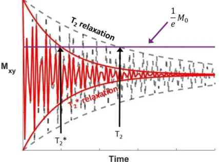
𝑇₂∗ _{“Observed” T}

2 in the presence of magnetic field inhomogeneities (s)

TE Echo time (s)

TM Mixing time (s)

TR Repetition time (s)

Tukey’s HSD Tukey’s Honest Significant Difference

𝑉 Blood velocity

(29)

28 Structure

19_F _Fluorine

1_H _Proton

BBB Blood brain barrier

Ctx Cortex

Gd Gadolinium

GM Grey matter

Hp Hippocampus

ICA Internal carotid arteries

LC Left cortex

LT Left thalamus

RBC Red blood cell

St Striatum

WM White Matter

Others

AD Alzheimer’s disease

APP Amyloid precursor protein FITC Fluorescein isothiocyanate NMR Nuclear magnetic resonance NSF Nephrogenic systemic fibrosis

O2 Dioxygen

PO2 Intravascular oxygen level

PS1 Presenilin 1

(30)

29

General introduction

The brain is one of the most important organs in the human body. Its structural and functional integrity requires a continuous supply of energy, oxygen and glucose, mediated by circulating blood flow. The microvasculature, particularly the capillary network, is directly responsible for oxygen transport to the tissue and the regulation of local blood flow. A good understanding of the microcirculation is an essential aspect necessary to obtain the perfusion patterns in healthy and diseased tissues. The microcirculation can be visualized and studied using medical imaging. The term medical imaging refers to techniques and processes that create images of the inside of the body which can help the medical staff to diagnose a disease, follow the evolution of a treatment, guide the surgeon during a medical intervention and help study tissues and organs in vivo. Several types of imaging techniques exist. Compared to other imaging techniques able to image the whole body, computed tomography and positron emission tomography, magnetic resonance imaging (MRI) uses no ionizing radiation and is relatively non-invasive. MRI can study hydrogen as well as other nuclei such as carbon 13, sodium 23, etc. The nucleus the most commonly studied is however hydrogen because of its abundance in the human body. Several MRI techniques gathered under the term MRI angiography can be used to observe the large blood vessels such as arteries and veins. However, to study microvessels, the spatial resolution of MRI does not allow for their direct visualization. Nevertheless, with a well-chosen design of the pulse sequence, MRI can be made sensitive only to protons in motion inside the body. This motion is restricted by natural barriers such as cell membranes, vessel walls and macromolecules. One particularly interesting MRI technique to extract information from the microvasculature is the IntraVoxel Incoherent Motion (IVIM) technique. It is able to differentiate between water protons inside the tissue and inside the microvasculature. IVIM is capable of giving macroscopic information about microscopic processes, namely flow inside the microvessels. Moreover, it has numerous substantial advantages over other similar techniques as it is free from contrast agent injection, completely noninvasive and easy to implement on a clinical scanner as based on a standard MRI sequence available on every clinical scanner from any manufacturer.

(31)

30 However, although it has been proven that IVIM is sensitive to flow in the microvasculature, it is not clear if it is sensitive only to the capillary network or to a larger part of the microvasculature. If the second hypothesis is correct, it could enlarge the scope of the applications opened to IVIM. The goal of this thesis is to better understand from where the IVIM signal originates, validate our hypothesis experimentally and apply the IVIM technique to the study of an animal model of Alzheimer’s disease.

The first chapter of this manuscript provides a brief description of the blood content and the brain microvasculature. In Chapter 2, the basics of MR physics are presented and applied to define and compare the MRI techniques which can be used to study blood flow in the brain. The advantages of the IVIM technique over the other MRI techniques are exposed at the end of this chapter. The validity of the standard IVIM signal model is challenged in Chapter 3 and a bi-exponential IVIM model accounting for two distinct vascular pools is found to better describe the IVIM signal experimentally at short diffusion times. Mathematical modelling of the IVIM signal is then performed in Chapter 4 to design numerical simulations of the IVIM signal. These simulations are used in Chapter 5 to create a dictionary of simulated signals which is then compared to the signals obtained experimentally in order to extract structural information about the two vascular pools of the proposed bi-exponential IVIM model. The influence of acquisition parameters on the IVIM signal is also investigated in Chapter 5. IVIM is then applied to the study of an animal model of Alzheimer’s disease in Chapter 6. The final chapter, Chapter 7, contains the conclusions, possible improvements and future work of this thesis.

(32)

31

Chapter 1: Blood vessels in the brain

This chapter introduces the brain vasculature, first by defining blood constituents, then introducing the brain vascular architecture before focusing on the brain microvasculature. Finally, the last section describes how the microvascular network can be modelled and simulated.

1.1 Blood content

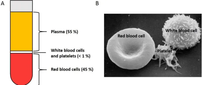
Blood is the most important fluid in the human body. This section presents the main functions of blood by going through its main constituents. As shown in Figure 1.1.A, the major components of blood are plasma (~ 55 %), red blood cells (RBCs) (~ 45 %), white blood cells and platelets (< 1 %).

Figure 1.1. (A) Blood content represented in a centrifuged tube of blood sample. The heavier components, the red blood cells, pack at the bottom of the tube. Just above are the white blood cells and platelets. Finally, the principal component of blood, plasma, stays on top. (B) Scanning electron microscopy image of a red blood cell, platelet and white blood cell. Image taken at the Electron Microscopy Facility at the National Cancer Institute at Frederick, Maryland, USA.

1.1.1 Plasma

Plasma is the yellow fluid that remains after centrifuging a blood sample. It carries all the blood constituents to the cells. Apart from RBCs, white blood cells and platelets, it also contains sugars, lipids, vitamins, minerals, hormones, enzymes, antibodies and other proteins.

(33)

32 1.1.2 Red blood cells

RBCs, also called erythrocytes, account for 45 % of the blood content. As shown in the scanning electron microscopy image in Figure 1.1.B, they look like flattened biconcave discs of about 7 µm in diameter. They have no nucleus. Their purpose is the transport of dioxygen, O2, from the lungs to every cell in the body and of carbon dioxide from the cells back to the lungs. To accomplish that, RBCs have each around 280 million hemoglobin proteins. Hemoglobin consists of 4 hems, each containing one iron atom. Hems are arranged to leave a caveat at the center of the protein. The quaternary structure of the hemoglobin is important for the capture of O2 or its release. Figure 1.2 shows the two possible conformation states of the hemoglobin protein in quaternary structure: state T (for tensed) and state R (for relaxed).

Figure 1.2. Transition between T and R states of hemoglobin in quaternary structure representation. The 4 hems of hemoglobin are also called subunits: 1, 2, here in grey and 1 and 2, here in blue. Histidine residues (His HC3) located at one end of the  subunits rotate between T and R states to the center of the caveat. This and other mechanisms result in a narrowing of the caveat of the hemoglobin in R state. This state is preferred when binding O2. From Leningher [2].

At low pH and concentration of O2, the protein is preferably in T conformation which has low affinity for O2. Thus, if an O2 molecule was attached to the protein, it is released. On the contrary, if the pH is high as well as the O2 concentration, the R conformation with more affinity to O2 is preferred and hemoglobin is able to bind to O2. In fact, the T conformation is more

(34)

33 stable than the R conformation but, when O2 is present, it stabilizes the R conformation. Patients suffering from anemia lack of RBCs and feel fatigued due to a shortage of oxygen. When oxygen binds to iron atoms in hemoglobin, hemoglobin is called oxyhemoglobin and iron oxides are what gives blood its red color.

1.1.3 White blood cells

White blood cells, also called leukocytes, are about 600 times fewer than RBCs and represent less than 1% of the blood content with platelets. They are part of the immune system. Figure 1.1.B shows a scanning electron microscopy image of a white blood cell. Unlike RBCs, leukocytes have a nucleus. There are three types of leukocytes. The most abundant are granulocytes which have small particles called granules inside their cytoplasm. They include basophils which are involved in inflammatory reactions and eosinophils and neutrophils which digest, phagocytize, complexes formed by antibodies-antigens and bacteria, respectively. The second most numerous type of leukocytes is lymphocytes, small cells with a large round nuclei and a small cytoplasm, which are responsible for killing viruses and produce antibodies. The last category is monocytes which are precursors to macrophages which digest bacteria as well as viruses. Thus, blood also has the function to transport these cells of the immune system quickly to the location of an infection. White blood cells do not always stay inside the blood vessels and can easily cross the vessel walls by amoeboid motion. They are able to pass through holes in the vessel walls smaller than themselves by extending a small part of the cell called a pseudopodium through the vessel wall. The cell’s cytoplasm and content progressively stream to that pseudopodium and finally arrive in the surrounding tissue.

1.1.4 Platelets

Platelets are the smallest elements in blood and are actually fragments of larger cells found in the bone marrow. They have no nucleus. Resting platelets are smooth discs of 2-4 µm in diameter while upon activation they have an irregular shape with protruding pseudopodia as the one shown in Figure 1.1.B. In that state, they are capable of the same amoeboid motion as white blood cells. The role of platelets is to start the clotting when a blood vessel is damaged and they constitute the major mass of the clot. In some circumstances, platelets can also produce a circulating clot also called thrombosis which, if located in one of a major arteries, can

(35)

34 prevent blood from flowing into one part of the heart or the brain and cause a heart attack or a stroke, respectively.

As a conclusion, all blood constituents have their own function: blood, oxygen and nutrients transportation, infection fighting and blood clotting. They contribute to the well-being of the organs and any change in the blood content can have tremendous consequences on the viability of the organ.

1.2 The brain vascular system

1.2.1 Why does the brain need a constant vascular input?

The brain is the most complex organ of the body. In the early eighteenth century, it was discovered to consist of two different parts: the white matter (WM) and the grey matter (GM) [3]. The WM, which represents more than half of the brain [4], mainly consists of myelinated axons and very few neuronal cell bodies. Its function is to ensure electrical connections between neurons. The GM includes all neurons, dendrites, microglia, astrocytes and blood vessels and represents less than 50 % of the brain. The function of neurons is to process information received through dendrites or axons. Dendrites have the same role as axons but are not surrounded by myelin and are shorter than axons. Microglial cells are part of the immune system and fight against foreign materials. Astrocytes, located between neurons and blood vessels, transport nutrients from the blood vessels to the neurons and also support endothelial cells that form the blood brain barrier (BBB). The BBB is a physiological barrier designed to protect the brain by regulating the crossing of particles from the blood stream at the capillary level to the brain tissue.

The brain consumes 20 % of the total energy of the body even though it represents only 2 % of the total body weight [5]. However, this organ is not able to store energy. This is why the brain needs a constant vascular input. Figure 1.3 shows the brain vasculature with a brain for which the tissues surrounding the vessels have been dissolved. The brain is not the organ receiving the most part of the cardiac output at rest. The kidneys, liver, spleen, gastrointestinal tract and skeletal muscles are more vascularized than the brain.

(36)

35 Figure 1.3. Cerebral blood vessels obtained by injecting the blood vessels with a plastic emulsion and dissolving the brain parenchyma. From Zlokovic et al [6].

Blood vessels have the important function to provide organs with energy supplies and remove the waste products. A constant regulation of the supply and removal of these materials in the brain is needed otherwise a cascade of events is initiated which leads to neuronal deaths and irreversible damages [7].

1.2.2 Vasculogenesis and angiogenesis mechanisms

The first process to occur in vascular network generation is vasculogenesis. In the embryo, endothelial precursor cells (angioblasts) migrate and differentiate into endothelial cells to create a first network of blood vessels. Then angiogenesis takes place. This process is shown in Figure 1.4.A: perivascular cells detach from the vessel walls and the vessel membrane is degraded to allow migration of endothelial cells creating new vessel buds and sprouts. These buds and sprouts elongate and form branches before being stabilized by the recruitment of perivascular cells and the production of extracellular matrix compounds.

Vasculogenesis was thought to be only a pre-natal process but it can also occur in the adult organism by recruitment of circulating angioblasts as shown in Figure 1.4.B. For example, post-natal vasculogenesis is involved in wound healing [8], limb ischemia [9] and tumor growth [10].

(37)

36 Figure 1.4. Mechanisms of blood vessel formation. (A) Angiogenesis: 1) upon activation by pro-angiogenic growth factors, perivascular cells (in blue) detach from the vascular wall and endothelial cells (in red) release proteases, which degrades their basement membrane. 2) It allows for endothelial cells migration and the formation of vessel buds or sprouts. 3) These sprouts further elongate and make branches and interconnections. 4) The new blood vessels are stabilized by the recruitment of perivascular cells and the production of extracellular matrix compounds. (B) Post-natal vasculogenesis: vessels form from the recruitment of circulating angioblasts (in yellow), their proliferation and finally differentiation into mature endothelial cells. From Laschke et al [11].

1.2.3 Similarities between vascular and nervous systems

As blood vessels act as supply vessels for the neurons, their geometry is not random. Nerve fibers and blood vessels follow an orderly pattern, often alongside each other. They can influence each other’s development. Similarities have been found between the molecules involved in the guidance of nerve fibers and blood vessels and the growth factors directing angiogenic sprouting and those regulating terminal axon arborization [12]. Zheng et al. showed that there is a regional organization of the microvessels corresponding to the underlying organization of the neurons inside the primate visual cortex. They also suggest that this pattern can be generalized to other animals [13]. There is a close connection between the vascular and neuronal networks. The study of the vascular network can allow for a better understanding of

(38)

37 the organization of the neurons. Abnormalities in the nervous system most probably result or come from abnormalities in the vascular system.

1.2.4 Anatomy of the brain vascular system

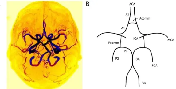
The human brain has approximately 400 miles of blood vessels. As it is the most important organ in the human body, its vascular system is the one which develops first in the embryo [14]. Blood arrives to the brain mainly from the two internal carotid arteries (ICA). It can also arise from the vertebral arteries which merge to form the basilar artery and join the ICA at the circle of Willis shown in Figure 1.5. Even if one artery is blocked or damaged, the circle of Willis enables to still provide normal cerebral perfusion as the arteries are all connected through that circle also called polygon. However, only about a half of the human population has a complete Willis polygon [15]. An incomplete polygon can condition the appearance and severity of cerebrovascular disorders such as aneurysms and infarctions.

Figure 1.5. (A) Axial maximum intensity projection time-of-flight (TOF) images of a complete circle of Willis from one patient. The TOF technique will be presented later in section 2.3.1. (B) Arteries comprising the circle of Willis. ICA: internal carotid artery; ACA: anterior cerebral artery; MCA: middle cerebral artery; PCA: posterior cerebral artery; BA: basilar artery; VA: vertebral artery; Acomm: anterior communicating artery; Pcomm: posterior communicating artery; A1, A2, P1, P2: branches of the anterior and posterior cerebral arteries. From Ezzatian-Ahar et al. [16] and Cucchiara et al [17].

From the circle of Willis, the anterior, middle and posterior cerebral arteries supply the brain with O2 and nutrients (Figure 1.5.B). If we focus for example on the cortex, the arteries which

(39)

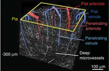
38 are mapping the surface of the cortex are called pial arteries. Smaller diameter arteries are named arterioles. When arterioles perforate the surface of the cortex, they are called penetrating arterioles and as they divide and their diameter decreases, they become deep microvessels or capillaries. Then capillaries merge to become venules which in turn merge to give veins which finally go back to the heart as the vena cava. Figure 1.6 shows a 3D reconstruction of a part of the cortex with the vascular network going from pial arterioles to pial venules.

Figure 1.6. 3D-reconstruction of a block of tissue collected by in vivo two-photon laser scanning microscopy from the upper layers of the mouse cortex. Penetrating vessels plunge into the depth of the cortex, bridging flow from surface vascular networks to capillary beds. From Shih et al [18].

1.2.5 Characteristics of the vessels

The two main parameters measured when studying the brain vascular network are the cerebral blood flow (CBF) and cerebral blood volume (CBV). These two parameters can be broken up at the vessel scale into three other parameters: the vessel diameter, the vessel length and the blood velocity. Table 1.1 gives estimates of these three parameters and the wall thickness for the different vessel types. In this table, arterioles, capillaries and venules have been gathered under the term microvessels. They will be described in more details in the next section.

(40)

39

Vessel type Vessel diameter (mm) Wall thickness (µm) Vessel length (cm) Blood velocity (mm/s) Aorta 25 1500 40 630 Large arteries 6.5 1000 20 200-500 Main artery branches 2.4 800 10 / Terminal artery branches 1.2 125 1 50 Microvessels 0.008-0.15 1-20 0.1-0.2 0.2-5 Terminal veins 1.5 10 1 / Main venous branches 5 100 10 / Large veins 14 200 20 / Vena cava 30 400 40 135

Table 1.1. Characteristics of the human blood vessels categorized by vessel type: vessel diameter, wall thickness, vessel length and blood velocity. From Freitas [19].

The vessel diameter displayed in Table 1.1 is the lumen diameter. Arteries have a smaller lumen diameter than veins because their wall thickness is thicker than the one of veins. Indeed, arteries’ membranes must resist high blood pressure changes. Then, pressure drops when blood passes through the capillaries and is very low inside the veins which thus have thinner vessel walls. The values provided for the vessel length and blood velocity in Table 1.1 are mean values.

1.3 The brain microvasculature

This thesis is centered on the study of the microvasculature which consists of the smallest vessels: capillaries, arterioles and venules (Figure 1.7).

First, techniques to extract structural information from the microvasculature are presented. Then, information about the geometry, structure and flow in the microvessels are summarized. Finally, methods to simulate the microvascular network are described.

(41)

40 Figure 1.7. 3D volume rendering of a selected zone of the cortex by scanning electron microscope showing the microvasculature: pial, penetrating arterioles and venules and capillaries. From Schoonover [20].

1.3.1 Methods to observe and extract information from the microvasculature

The main techniques having enough spatial resolution to visualize and extract structural parameters from the microvessels are performed postmortem, ex-vivo. These techniques involve two steps. Microvessels are usually labelled to enhance their contrast compared to the surrounding tissue before being imaged. Techniques to measure the blood velocity are different as they require in-vivo access. They will presented in section 1.3.3.1.

1.3.1.1 Staining of the blood vessels

Labeling of the microvessels is an important step to facilitate their visualization in the imaging step. Different strategies can be used.

A low viscosity resin like methyl methacrylate can be injected into the vessels replacing blood. After some time, it solidifies. Then, potassium hydroxide can be used to completely dissolve the surrounding tissue leaving the resin intact and yielding a cast of vessels [21]. The advantage of this technique is that the vessels are completely separated from the tissue and they are not deformed so precise measurements of the lumen diameter can be obtained. However, as the vessels are no longer supported by nervous tissue, they are more difficult to identify.

(42)

41 The other staining techniques rely on histological methods. The most common method involves injection of india ink and gelatin [21], [22]. This method has the advantage to completely fill the microvascular network and allows for the precise identification and detailed study of arteries and veins. However, vascular rupture can happen in superficial vessels masking them. Also, the fixation and dehydration of the tissue following the injection of india ink can deform the vessels to a large extent making the measure of the vessel diameter not fully reliable. In addition to this, when some vessels are ruptured consequently to a disease, the ink can diffuse outside of the vessel.

Another strategy consists in injecting gelatin and fluorescein conjugated to albumin [23]. Crosslinking of the albumin to the gelatin skeleton prevents diffusion of the fluorophore in the extravascular space, even in exposed vessels. A derivative of the fluorescein, the fluorescein isothiocyanate (FITC), is often used in combination with dextran [24]. The india ink and fluorescein methods also permit simultaneous staining of other structures than the vessels. For example, if information about the location of the neurons compared to the vessels is sought, a fluorescent stain, DAPI, can be added to label all cell nuclei along with -NeuN antibody which allows for the differentiation of neuronal versus non-neuronal cells [23].

The two histological methods presented previously fill the vessels with a substance to label them. Another approach is to directly label endothelium cells of the vessel walls. This can be achieved by incubating the fixed tissue of interest with the calcium cobalt method to label alkaline phosphatase activity in the endothelium of blood vessels [25]. However, this type of staining is not homogeneous throughout the vascular tree [26]. In particular, venous capillaries are poorly stained. Other dyes use similar labeling strategies. Nissl targets the rough endoplasmic reticulum and free polyribosomes in neurons, glia and endothelial cells [27]. Von Willebrand factor specifically marks endothelial cells using specific antibodies [28]. And Dil efficiently stains the vessel membrane due to its lipophilic characteristics [29].

An interesting strategy is to combine staining of the perfused capillaries using for example FITC-dextran dyes with staining of the membranes of all capillaries by labeling alkaline phosphatase

(43)

42 activity in the endothelium of the vessels [30]. This allows for the comparison of perfused and non-perfused capillaries at the same time.

1.3.1.2 Imaging after staining of the blood vessels

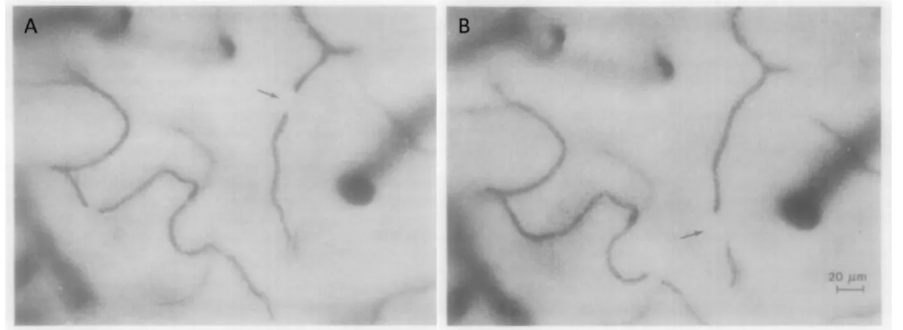
Several imaging techniques can be used to visualize the blood vessels after that they have been stained. Two-photon laser scanning microscopy (TPLSM) allows for the observation of fluorescent dyes such as fluorescein or FITC. Figure 1.8.A shows a TPLSM image of the mouse brain cortex with different fluorescent stains: DAPI, fluorescein and -NeuN. Blinder et al. managed to image the cortex with a 1 µm resolution [31]. However, this technique is limited by the imaging field and penetration depth of two-photon imaging.

Figure 1.8. (A) Maximal projection of two-photon laser scanning microscopy image data of a 2 mm region of the mouse brain cortex from the bregma. DAPI, fluorescein and -NeuN are fluorescent dyes of all cell nuclei, blood vessels and neuronal cells, respectively. (B) Light sheet microscopy image after india ink staining of a section of the human brain cortex showing the four cortical vascular layers (1-4) and examples of bush-like venous network (5-7) (x 64). (C) Scanning electron microscopy image of a cast of vessels of the human brain cortex. (1) Recurrent branch coupled with the parent vessel (2). Arrows indicate impressions of endothelial cell nuclei on the arterial cast (x 440). From Tsai et al. [23] and Duvernoy et al [21].

Light sheet microscopy (LSM) is generally used to image tissues stained with india ink or Nissl [22]. Figure 1.8.B is an example of a light sheet microscope image after injection of india ink and fixation of the sample. This optical method has the same limitations as TPLSM. However, a

(44)

43 technique to improve the penetration depth called optical clearing aiming to make the surrounding tissue transparent is more and more used [32]. For example, by adding liquid paraffin to a sample already stained with india ink, Hashimoto et al. managed to get whole mouse brain images with a 5 µm resolution [33].

To obtain LSM images, first the sample needs to be cut in very thin slices using a microtome. Techniques have been developed to perform this step at the same time as collecting the images. Li et al. created the micro-optical sectioning tomography (MOST) [34]. Using Nissl staining coupled with MOST, Wu et al. imaged the whole mouse brain at one micron voxel resolution with high image quality [35]. Xue et al. managed to get even better resolution with india ink perfusion: 0.35 x 0.4 x 2 µm3_{[36]. Another similar technique developed approximately at the} same time is knife-edge scanning microscopy (KESM) [37]. It allows to cut sections as thin as 0.5 µm from tissues embedded in resin with india ink or Nissl staining [38].

Casts of vessels obtained by dissolving tissues after filling the blood vessels with a resin are imaged with scanning electron microscopy (SEM) [21], [39]. Figure 1.8.C shows a SEM image of a vessel cast of the human brain cortex. Nuclei of endothelial cells are pointed at by arrows. SEM has higher resolution than light sheet microscopy and the depth of focus is high enough to get a large field of view enabling to reliably trace individual vessels either over very short or over extremely long distances.

Other strategies not using optical methods but MRI and CT can also be employed. Instead of injecting gelatin doped with gadolinium chelates to enhance the contrast in MRI images, an inert silicon rubber can be used. This other contrast agent causes vessels to appear dark on MRI and bright on CT. The low viscosity of the inert silicone rubber allows for complete filling of the vasculature and its hydrophobicity restricts itself from crossing the vessel membrane. By combining MRI and CT images, Dorr et al. created a whole brain mouse vascular atlas with a 30 µm resolution [40]. This staining is also suitable for optical imaging as the silicon rubber is optically opaque. Pathak et al. thus compared MRI and CT images with LSM images of the same mouse brain to show that good agreement can be obtained between the three techniques (Figure 1.9) [41].