RESEARCH OUTPUTS / RÉSULTATS DE RECHERCHE
Author(s) - Auteur(s) :
Publication date - Date de publication :
Permanent link - Permalien :
Rights / License - Licence de droit d’auteur :
Bibliothèque Universitaire Moretus Plantin
Institutional Repository - Research Portal
Dépôt Institutionnel - Portail de la Recherche
researchportal.unamur.be
University of Namur
Generating French virtual commuting networks at the municipality level
Lenormand, Maxime; Huet, Sylvie; Gargiulo, Floriana
Published in:Journal of Transport and Land Use
DOI:
10.5198/jtlu.v7i1.360
Publication date:
2014
Document Version
Publisher's PDF, also known as Version of record
Link to publication
Citation for pulished version (HARVARD):
Lenormand, M, Huet, S & Gargiulo, F 2014, 'Generating French virtual commuting networks at the municipality level', Journal of Transport and Land Use, vol. 7, no. 1, pp. 43-55. https://doi.org/10.5198/jtlu.v7i1.360
General rights
Copyright and moral rights for the publications made accessible in the public portal are retained by the authors and/or other copyright owners and it is a condition of accessing publications that users recognise and abide by the legal requirements associated with these rights. • Users may download and print one copy of any publication from the public portal for the purpose of private study or research. • You may not further distribute the material or use it for any profit-making activity or commercial gain
• You may freely distribute the URL identifying the publication in the public portal ?
Take down policy
If you believe that this document breaches copyright please contact us providing details, and we will remove access to the work immediately and investigate your claim.
http://jtlu.org
. 7 . 1 [2014] pp. 43–55 doi: 10.5198/jtlu.v7i1.360
Generating French virtual commuting networks at the municipality level
Maxime Lenormand IRSTEAa Sylvie Huet IRSTEA Floriana Gargiulo University of Namur
Abstract: We aim to generate virtual commuting networks in the rural regions of France in order to study the dynamics of their municipalities. Since it will be necessary to model small commuting flows between municipalities with a few hundred or thousand inhabitants, we have opted for the stochastic model presented byGargiulo et al.(2012). is model reproduces various possible complete networks using an iterative process, stochastically selecting a workplace in the region for each commuter living in the municipality of a region. e choice is made con-sidering the job offers in each municipality of the region and the distance to all of the possible destinations. is paper will present methods for adapting and implementing this model to generate commuting networks between municipalities for regions in France. We address three different issues: How can we generate a reliable virtual commuting network for a region that is highly dependent on other regions for the satisfaction of its residents’ demands for employment? What about a convenient deterrence function? How can we calibrate the model when detailed data is not available? Our solution proposes an extended job search geographical base for commuters living in the municipalities; we compare two different deterrence functions and we show that the parameter is a constant for network linking municipalities in France. 1 Introduction
e connection between the home and workplace plays a cen-tral role in understanding the socio-economic relations in a network of rural municipalities (Clark et al. 2003;Reggiani and Rietveld 2010). Indeed, new economic theories assume local positive dynamics can be explained by implicit geograph-ical money transfers made by commuters or retired people (see for example Davezies (2009)). Simulation is becom-ing an increasbecom-ingly convenient tool to study populations and their interactions over space. at is particularly the case with individual-based approaches, which allow for the study of the-ories at the individual level since they simulate the variations in how individuals interact with each other and with their en-vironment. Recent modeling reviews show the increasing use of such a tool (Birkin and Wu 2012;Bousquet and Page 2004;
Parker et al. 2003;Rindfuss et al. 2004;Verburg et al. 2004;
Waddell et al. 2003). However, these approaches require gen-eration models capable of building reliable virtual commuting networks that consider each individual within a population. at is the case in the SimVillages dynamic micro-simulation model we developed during the PRIMA¹project. Indeed, in the SimVillages model, aer generating a synthetic population of individuals (Gargiulo et al. 2010), it is necessary to choose a
¹ PRototypical policy Impacts on Multifunctional Activities in rural municipalities - EU 7th Framework Research Programme; 2008-2011;
https://prima.cemagref.fr/the-project
place of work for each worker within this population because a commuting origin-destination table was unavailable.
e goal of the European PRIMA project was to under-stand the dynamics of rural municipalities in France. Ninety-five percent of them have fewer than 3000 inhabitants. is means that most of the commuting flows we want to study are weak, with a spatial distribution very difficult to predict with the available variables at an aggregated level. is is why we opt for the stochastic model recently proposed byGargiulo et al.(2012). Moreover, we want to consider the commuting network on different dates. Detailed data regarding flows be-tween pairs of municipalities are only available in France for the year 1999. For other years, the only reliable data is aggre-gated data for each municipality, which describes how many people work outside of the municipality and how many come from outside of the municipality to work. Such data lacks precision regarding the various places of work and the various municipalities where citizens reside. en we also choose the
Gargiulo et al.(2012) model for its ability to generate a pop-ulation of individuals on a commuting network, starting from this data. is model reproduces the complete network us-ing an iterative process that stochastically selects a workplace in the region for each commuter living in the municipality of the region. e choice is made while considering the job of-fers in each municipality of the region and the distance to all possible destinations. It differs from the classical generation models presented inOrtúzar and Willumsen(2011) since it is
Copyright 2014 Maxime Lenormand, Sylvie Huet, and Floriana Gargiulo.
. a discrete choice model where the individual decision function
is inspired by the gravity law model, which is not usually em-ployed on an individual level (Barthélemy 2011;Haynes and Fotheringham 1984;Ortúzar and Willumsen 2011). More-over, such a model ensures that for every municipality the vir-tual total numbers of commuters both coming in and going out are the same as the ones supplied by the data.
is paper presents a method to adapt and implement this model to generate commuting networks between municipali-ties for regions in France. is implementation has forced us to address three different issues: How can we generate a re-liable virtual commuting network for a region highly depen-dent on other regions to satisfy the need for jobs for the people living in the municipalities? What about a convenient deter-rence function? How should the model be calibrated when detailed data is not available?
e first problem to solve involves the fact that regions in France are not islands, as presented in the example ofDe Mon-tis et al.(2007,2010). Indeed, some of the inhabitants, espe-cially those living close to the borders of the region, are likely to work in municipalities located outside the region of resi-dence. is part of the population, especially if it is signifi-cant, causes the generated network to register false if we only consider that people living in the region also work in the re-gion. A method for solving this problem involves generating the commuting network only for people living and working in the region. However, in order to do this the modeler must know the quantity and the place of residence for individuals who work outside but live within the region. Data providing this information is very rare. erefore, we address this issue by extending the job search geographical base for commuters living in the municipalities to a sufficiently large number of municipalities located outside the region of residence. en, we compare the model that does not include outside munici-palities to the model including outside municimunici-palities in 23 re-gions in France and come to a conclusion regarding the quality of our solution.
e second problem relates to the form of the deterrence function, which governs the impact of distance on the choice of the place of work relative to the quantity of job offers. e initial work done byGargiulo et al.(2012) proposes the use of a power law. However,Barthélemy(2011) states that the form of the deterrence function varies greatly and can sometimes be inspired by an exponential function, such as inBalcan et al.
(2009), or by a power law function as inViboud et al.(2006). To choose the much more convenient deterrence function, we have compared the quality of generated networks for 34 re-gions in France obtained with both the exponential law and
the power law. Better results were obtained with the expo-nential law.
e final problem was related to calibration. e gener-ation model, as with most of the currently used commuting network generation models, has one parameter to calibrate. is parameter governs the impact of distance on the individ-ual decision regarding the place of work relative to the quan-tity of job offers. is parameter was calibrated through min-imization of the Kolmokorov-Smirnov distance between the observed and simulated commuting distance distribution for individuals of the studied region. When detailed data is not available, it is necessary to find a way to determine this param-eter. e only available distance that can be used is the Eu-clidian distance. While detailed commuting network data was available for the year 1999 and could be used for calibration, it was not available for earlier or more recent years. ough it may be possible to assume the parameter value does not change over time, a transportation network can evolve greatly at the local level to reduce the time distance. Such a change cannot be recorded when using the Euclidian distance. A solution was finally found. Using 34 regions in France, we show that every region can be generated using a constant value for the parame-ter. en, we assume that the parameter value is constant over time and space.
2 Material and methods
2.1 The French case studies and data from the French statistical office
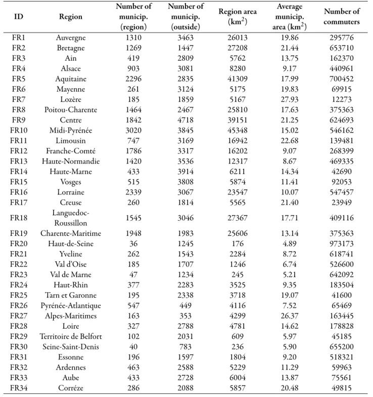
A complete description of the regions from which the network was generated is provided in Table4. ese regions have been randomly chosen for their diversity in terms of number of mu-nicipalities, number of commuters and surface areas. Some correspond to an administrative region of France while oth-ers are closer to the county (known as “departments,” a French administrative unit). ese two types of case studies are called “region” hereaer.
e French Statistical Office (INSEE) collects information regarding each individual’s residence and place of work.²From this collected data, the Maurice Halbwachs Center or INSEE makes the following data available for every researcher:
1. In 1999, the observed commuting networks, i.e., data re-garding the numbers of individuals commuting from
lo-² INSEE (Institut National de la Statistique et des Etudes Economiques, Recensement de la population française : tableaux ”mobilités” - France
entière - 1999, CMH | lil-0257,http://www.reseau-quetelet.cnrs.fr/spip/
Generating French virtual commuting networks (in press) cationi to location j for every municipality of a region
(called “observed data” hereaer);
2. In 1999, the total number of commuters, the total job offers, and the total number of workers in residence for every municipality. ese data allow computations to be made for the number of workers that commute to their place of employment for each municipality.
3. e Lambert coordinates for each municipality are easy to find on the Internet. ey are used to compute the Euclidian distance between each pair of municipalities. We used the data sets 2 and 3 as inputs of the algorithms described in this paper to simulate commuting networks (S).
We compare these simulated commuting networks to “real” network (R) built from the observed data of the data set 1.
2.2 TheGargiulo et al.(2012) model
Consider a region composed of n municipalities. We can
model the observed commuting network starting from ma-trixR∈ Mn×n(N), where Ri jrepresents the number of com-muters from municipalityi (in the region) to municipality j
(in the region). is matrix represents the light gray origin-destination table presented in Table1.
e inputs of the algorithm are:
• D = (di j)1≤i,j≤n the Euclidean distance matrix
be-tween municipalities.
• Ij, the number of in-commuters from the region to mu-nicipalityj of the region, 1≤ j ≤ n (i.e., the number of
individuals living in the region in municipalityi (i̸= j)
and working in municipalityj ).
• Oi, the number of out-commuters from municipalityi of the region to the region, 1≤ i ≤ n (i.e., the number of individuals working in the region in municipality j
(j̸= i) and living in municipality i).
Ik andOkcan be respectively assimilated to the job offers for those employed in the region and the job demand of those employed in the region for municipalityk, 1≤ k ≤ n. e
algorithm starts with:
Ij= n ∑ i=1 Ri j (1) and Oi= n ∑ j=1 Ri j (2)
e purpose of the model is to generate the light gray origin-destination sub-table of the region described in Table1. To do this it generates matrixS∈ Mn×n(N) where Si j repre-sents the number of commuters from municipalityi (in the
re-gion) to municipalityj (in the region). It’s important to note
thatSi j= 0 if i = j. e algorithm assigns to each individual
a place of work with a probability based on the distance from the place of residence to every possible place of work and their corresponding job offer. e number of in-commuters for municipalityj and the number of out-commuters for
munici-palityi decrease each time an individual living in i is assigned
municipalityj as a workplace. e algorithm is stopped when
all out-commuters have a place of work. e algorithm is de-scribed in Algorithm2.1withm= n.
Algorithm 2.1 Commuting generation model Input : D∈ Mn×m(R), I ∈ Nm,O∈ Nn,β ∈ R + Output : S∈ Mn×m(N) Si j ← 0 while∑ni=1Oi> 0 do Simulatei∼ UAwhereA= {k|k ∈ |[1, n]|, Ok̸= 0}
Simulate j from|[1, m]| with a probability:
Pi→j =∑mIjf(di j,β) k=1Ikf(di k,β) Si j ← Si j+ 1 Ij ← Ij− 1 Oi← Oi− 1 end while return S
Gargiulo et al.(2012) uses deterrence function f(di j,β) with a power law shape:
f(di j,β) = di j−β 1≤ i, j ≤ n . (3)
3 Statistical tools
is section presents the tools used to calibrate the model and to compare various implementation choices.
3.1 Calibration of theβvalue
e same method used inGargiulo et al.(2012) is used to cal-ibrate theβ value. e β value is calibrated so as to minimize the average Kolmogorov-Smirnov distance between the simu-lated commuting distance distribution and one building from
.
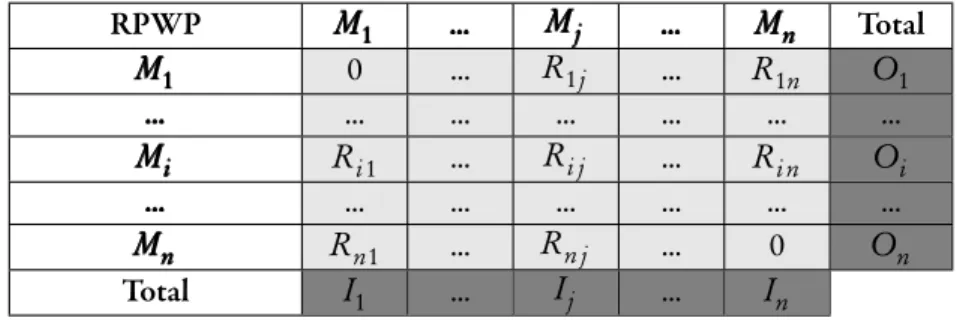
Table 1:Origin-destination table for the region; e light gray table represents the commuters living (place of residence RP) and working (place of work WP) in the region for each municipality of the region; e dark gray line represents the number of out-commuters from municipality of the region to the region for each municipality of the region (i.e., the row totals of the light gray table); e dark gray column represents the number of in-commuters from the region to a municipality of the region for each municipality of the region (i.e., the column totals of the light gray table).
RPWP MMM111 ... MMMjjj ... MMMnnn Total M1 MM11 0 ... R1j ... R1n O1 ... ... ... ... ... ... ... ... ... MMMiii Ri1 ... Ri j ... Ri n Oi ... ... ... ... ... ... ... ... ... MMMnnn Rn1 ... Rn j ... 0 On Total I1 ... Ij ... In RPWP MMM111 ... MMMjjj ... MMMnnn Total M1 MM11 0 ... R1j ... R1n O1 ... ... ... ... ... ... ... ... ... MMMiii Ri1 ... Ri j ... Ri n Oi ... ... ... ... ... ... ... ... ... MMMnnn Rn1 ... Rn j ... 0 On Total I1 ... Ij ... In
the observed data. For the basic model we compute the com-muting distance distribution with the comcom-muting distance of individuals who are commuting from the region to the re-gion. For the model focused on the outside area, we compute the commuting distance distribution with the commuting dis-tance of the individuals who are commuting from the region to the region and the outside area.
As theGargiulo et al.(2012) model is stochastic, the final calibration value we consider is the averageβ value over 10 replications of the generation process.
3.2 An indicator to assess the change
It is necessary to have an indicator to compare the simulated commuting network and the observed commuting network (data set 1 in section2.1). LetR∈ Mn
1×n2(N) represent the
observed commuting network whenRi jrepresents the num-ber of commuters from municipalityi to municipality j . Let
S ∈ Mn
1×n2(N) represent a simulated commuting network
for the same municipalities. We can calculate the number of common commuters betweenR and S (Eq.4) and the num-ber of commuters inR (Eq.5):
NC Cn1×n2(S, R) = n1 ∑ i=1 n2 ∑ j=1 min(Si j,Ri j) (4) NCn1×n2(R) = n1 ∑ i=1 n2 ∑ j=1 Ri j (5)
From Eq.4and Eq. 5we calculate the Sørensen similarity index (Sørensen 1948). is index is suitable because it corre-sponds to the common part of commuters betweenR and S.
us it is called the common part of commuters (CPC) (Eq.
6):
C P Cn1×n2(S, R) = 2NC Cn1×n2(S, R)
NCn1×n2(R) + NCn1×n2(S) (6)
is index has been chosen for its intuitive explanatory power, as it is a similarity coefficient that provides the like-ness degree between two networks. e index ranges from a value of zero, for which there are not any commuter flows in common in the two networks, to a value of one, when all com-muter flows are identical between the two networks.
4 Generating commuting networks for French regions at the municipality level
4.1 How to cope with regions that are not islands or those that lack detailed data?
A commuting network is defined by an origin-destination ta-ble (light gray tata-ble in Tata-ble2). At the regional level, this means that it is necessary to know, for each municipality of residence and for each municipality of employment, the value for the flow of commuters traveling from one to another. is kind of data is not always provided by statistical offices and the datasets are usually aggregated: only the total number of out-commuters and in-out-commuters for each municipality is avail-able for each (dark gray row and column in Tavail-able2). To apply the model and define the commuting network, unless we are
Generating French virtual commuting networks (in press) in a significantly isolated region³, we need to find a way to
iso-late from the total number of in(out)-commuters (dark gray row and column in Table2) the fraction that relates strictly to the region (light gray table in Table2). However, this is not a simple task.
Furthermore, even if these parts can be isolated, a problem remains due to the border effect. Indeed, if we consider only the region, there is the risk of making an error in the recon-struction of the network for municipalities near the region’s border. e higher the proportion of individuals working out-side of the region, the more significant the error will be.
To go further, we propose to change the inputs for the algo-rithm. Instead of only considering the regional municipalities as possible places of work, we also consider an area outside of the region. e outside area represents the surroundings of the studied area. e following section describes a method for considering this outside area practically.
4.1.1 A new extended to outside job search base
We implement the model to generate 23 various regions in France. eir outside area is composed of the set of munici-palities of their neighboring ”departments.”
We consider the outside of the region to be composed of
m− n municipalities, where n represents the number of
mu-nicipalities in the region. e inputs are the directly available aggregated data at the municipal level:
• D = (di j)1≤i≤n
1≤j≤m, the Euclidean distance matrix between
municipalities both in the same region and in the outside area.
• (Ij)1≤j≤m, the total number of in-commuters of munic-ipalityj of the region and outside of it (i.e., the number
of individuals working in municipalityj of the region or
the outside area and living in another municipality).
• (Oi)1≤i≤n, the total number of out-commuters of mu-nicipalityi of the region only (i.e., the number of
indi-viduals living in municipalityi of the region and working
in another municipality).
e purpose of the algorithm that introduces the outside is to generate the origin-destination table (light gray and gray sub-table in Table2). To do this, the algorithm presented in Algorithm2.1is used to simulate Table3. From this, through difference Table2can be obtained with the total number of
³ An island, for example. In this case, the gray rows and columns in Table
2would not exist.
in-commuters(Ij)1≤j≤n, the total number of out-commuters (Oi)1≤i≤n, and the light gray table of Table3.
A matricial representation of the origin-destination table presented in the light gray and gray sub-table in Table 2, known as the simulated matrixS ∈ M(n+1)×(n+1)(N), is
ob-tained.Si jrepresents:
• the number of commuters from municipality i (in the
region) to municipalityj (in the region) if i, j̸= n + 1; • the number of commuters from the outside area to
mu-nicipalityj (in the region) if i= n + 1 and j ̸= n + 1; • the number of commuters from municipality i to the
outside area ifi̸= n + 1 and j = n + 1.
4.1.2 Comparison of the two models: Assessing the impact of the outside
We assess the impact of the outside area through a comparison between the network generations for 23 French regions both including and not including the outside area. e generation is made on a municipality scale using a power law deterrence function.
Both implementations are compared through their CPC values between the simulated network S and the observed
networkR (data set 1 presented in Section2.1) for each re-gion. We replicate the generation for each region 10 times and our indicator on each replicate is calculated. In all the presented figures, the indicator averages 10 replications. e variation of the indicator over the replications is very low, av-eraging 1.02 percent at most. Consequently, this is not rep-resented on the figures. Fig. 1presents the common part of commutersC P Cn×n(S, R) between the simulated network
S and the observed network R. e squares represent the
CPC between the observed networkR and the simulated
net-works obtained with the regional job search base. e tri-angles represent the CPC between the observed networkR
and the simulated networks obtained with a job search base comprising the region and its outside area. It’s important to note that for the implementation without the outside area,
S ∈ Mn×n(N), while for the implementation with the
out-side area, S ∈ M(n+1)×(n+1)(N). In order to compare the two models, the regional network (commuters from the re-gion to the rere-gion) must be taken into consideration. Indeed, in the without-outside-area cases,NCn×n(S) = NCn×n(R), but this is not necessarily true for the with-outside-area cases. Fig. 1shows that the two job search bases give results that are not different. us, introducing the outside area solves the
.
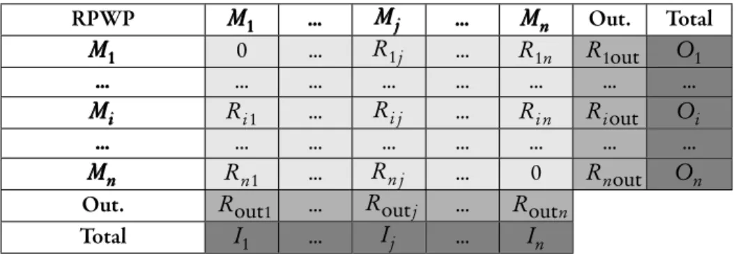
Table 2:Origin-destination table. e light gray table represents the commuters living and working in the region for each munic-ipality of the region. e gray column represents the out-commuters living in the region and working outside (Out.) for each municipality of the region. e gray line represents the in-commuters working in the region and living outside (Out.) for each municipality of the region. e dark gray line (column) represents the total number of out(in)-commuters for each municipality of the region.
RPWP MMM111 ... MMMjjj ... MMMnnn Out. Total M1 M1 M1 0 ... R1j ... R1n R1out O1 ... ... ... ... ... ... ... ... Mi MMii Ri1 ... Ri j ... Ri n Riout Oi ... ... ... ... ... ... ... ... Mn MMnn Rn1 ... Rn j ... 0 Rnout On
Out. Rout1 ... Routj ... Routn
Total I1 ... Ij ... In RPWP MMM111 ... MMMjjj ... MMMnnn Out. Total M1 M1 M1 0 ... R1j ... R1n R1out O1 ... ... ... ... ... ... ... ... Mi MMii Ri1 ... Ri j ... Ri n Riout Oi ... ... ... ... ... ... ... ... Mn MMnn Rn1 ... Rn j ... 0 Rnout On
Out. Rout1 ... Routj ... Routn
Total I1 ... Ij ... In
Table 3:Origin-destination table from the region to the region and the outside area. e light gray table represents the commuters living (place of residence, RP) and working (place of work, WP) in the region for each municipality of the region. e gray table represents the commuters living (place of residence, RP) in the region and working (place of work, WP) outside of the region. RPWP MMM111 ... MMMjjj ... MMMnnn MMMnnn+1+1+1 ... MMMmmm MMM111 0 ... R1j ... R1n R1n+1 ... R1m ... ... ... ... ... ... ... ... ... ... Mi MMii Ri1 ... Ri j ... Ri n Ri n+1 ... Ri m ... ... ... ... ... ... ... ... ... ... Mn Mn Mn Rn1 ... Rn j ... 0 Rnn+1 ... Rnm RPWP MMM111 ... MMMjjj ... MMMnnn MMMn+1n+1n+1 ... MMMmmm MMM111 0 ... R1j ... R1n R1n+1 ... R1m ... ... ... ... ... ... ... ... ... ... Mi MMii Ri1 ... Ri j ... Ri n Ri n+1 ... Ri m ... ... ... ... ... ... ... ... ... ... Mn Mn Mn Rn1 ... Rn j ... 0 Rnn+1 ... Rnm
Generating French virtual commuting networks (in press) 0.5 0.6 0.7 0.8 0.9 Common par t of comm uters FR1 FR2 FR3 FR4 FR5 FR6 FR7 FR8 FR9 FR10 FR11 FR12 FR13 FR14 FR15 FR16 FR17 FR18 FR19 FR20 FR21 FR22 FR23
Figure 1:Average CPC for 23 regions. e squares represent the basic model; the triangles represent the model with the outside area.
problem linked to a lack of detailed data without changing the quality of the resulted simulated network. Indeed, one must keep in mind that the inputs for the with-outside-area cases do not require detailed data in comparison to the without-outside-area cases.
4.2 Choosing a shape for the deterrence function
e next problem relates to the form of the deterrence func-tion which rules the impact of distance on the choice of the place of work relative to the quantity of job offers. e initial work done byGargiulo et al.(2012) proposes to use a power law. However,Barthélemy(2011) states the form of the de-terrence function varies significantly and can sometimes be in-spired by an exponential function as inBalcan et al.(2009) or by a power law function as inViboud et al.(2006). By choos-ing the much more convenient deterrence function, we com-pare the quality of generated networks for 34 French regions obtained with the model including the outside area using both the exponential law and the power law.
A deterrence function following an exponential law is in-troduced:
f(di j,β) = e−βdi j 1≤ i ≤ n and 1 ≤ j ≤ m . (7)
To compare the two deterrence functions, we have gener-ated the networks of 34 various French regions (see Table4
for details) that replicate 10 times for each region. e net-works were generated with a job search base for the algorithm that considers the outside area.
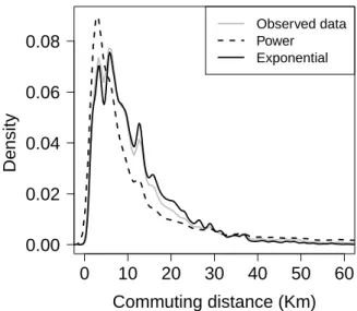
0 10 20 30 40 50 60 0.00 0.02 0.04 0.06 0.08 Commuting distance (Km) Observed data Power Exponential Density
Figure 2:Density of the Auvergne commuting distance distri-bution. e solid line represents the observed com-muting distance distribution; the dotted line repre-sents the commuting distance distribution obtained with the calibrated model with a job search base comprising the outside and the exponential law; the dashed line represents the commuting distance dis-tribution obtained with a job search base comprising the outside and the power law. e two simulated commuting distance distributions are computed for one replication each.
For example, Fig. 2shows that we obtained a better es-timation of the Auvergne commuting distance distribution when using the exponential law. We computed the observed commuting distance distribution with the observed Auvergne commuting network (data set 1 presented in Section2.1) and the Euclidean distances between the Auvergne municipalities (data set 3 presented in Section2.1).
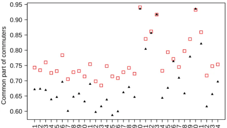
More systematically, we plot, for the exponential law and power law, the average of the replications for the common part of commutersC P C(n+1)×(n+1)(S, R) between the simulated
networkS and the observed network R in Fig.3. is clearly indicates that the average proportion of common commuters is always better when using an exponential law represented by squares.
4.3 Spatial analysis
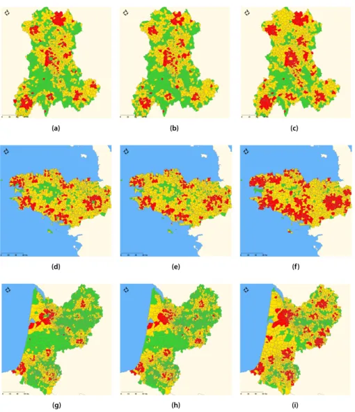
To better understand how CPC is spatially distributed at a more granular level, we mapped the CPC by municipality for three models and three study areas. In Fig. 4, it can be
ob- . 0.60 0.65 0.70 0.75 0.80 0.85 0.90 0.95 FR1 FR2 FR3 FR4 FR5 FR6 FR7 FR8 FR9 FR10 FR11 FR12 FR13 FR14 FR15 FR16 FR17 FR18 FR19 FR20 FR21 FR22 FR23 FR24 FR25 FR26 FR27 FR28 FR29 FR30 FR31 FR32 FR33 FR34 Common par t of comm uters
Figure 3:Average CPC for the power shape (triangle) and the exponential shape (square) for 34 French regions.
served that for all case studies (in rows) the highest values of the CPC were obtained by municipalities using the model with an exponential shape including the outside area (third column). It can also be noted that the model without the out-side area (second column) and the model with the power shape including the outside area (first column) give results that are not wholly different.
As we can see in Fig. 4, the CPC values are not uniformly distributed in the municipalities of the three areas. e error seems to increase as distance from the urban areas increases.
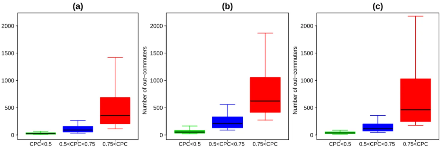
We now focus on the third model with an exponential shape including the outside area to better understand which types of municipalities compose the three clusters (CPC≤ 0.5, 0.5 <CPC≤ 0.75, and 0.75 <CPC). We identify the number of out-commuters as the most explanatory variable. Indeed, we can observe in Fig. 5that the distribution of the number of out-commuters in each cluster is significantly dif-ferent. e higher the average number of out-commuters, the higher the CPC. Having performed analyses of variance (ANOVA) for each case study, we obtained significant differ-ences between the averages for the number of out-commuters in each cluster with a 0.95 percent level of confidence for each case study.
For the three regions, the CPC value is strongly linked to municipality characteristics. Indeed, the municipalities with
0.75 <CPC are urban and suburban municipalities with a
high number of out-commuters that are close to a large ur-ban municipality. In contrast, the municipalities with a low number of out-commuters that are far from large urban nicipalities have a CPC lower than 0.5. For this type of
mu-nicipality, the commuting flows are very small. us they are difficult to reproduce with the mechanisms taken into consid-eration. However, the distance to cities does not appear to be particularly responsible for the error. e timing for the job offer arrival on the job market is probably much more signif-icant in determining the local topology of the network than elsewhere. ese flows represent about 4 percent of the total number of out-commuters for the Auvergne region, 1 percent for Bretagne, and 5 percent for Aquitaine.
4.4 Calibrating the model for French regions
e final problem involves the calibration process, which previously required detailed and accurate data.
Fig. 6shows the calibratedβ values for each of the 34 re-gions in France. It can be observed that these values display subtle variations from about 1.7· 10−4to 2.4· 10−4with the averageβ value (C = 1.94 · 10−4) corresponding to the dark line.
en we hypothesize that it is possible to directly calibrate the algorithm to generate the 34 regions in France by using a constant equal toC . To study the influence of this
approxi-mation on the common part of commuters, we have computed the CPC withC as the parameter value for the 34 regions. We
observe in Fig. 7that the influence of theβ value’s approxi-mation on the CPC is very weak. It can then be noted that the average CPC obtained withC is, for some regions, higher
than the CPC obtained by theβ value that is not averaged. It is possible that the common part of commuters is better with another beta value because it is not a calibration criterion.
It is not necessary to study the influence of theβ value’s approximation on the calibration criterion. Indeed, from the studies made byGargiulo et al.(2012), we know the CPC and the calibration criterion show a significant correlation. e CPC and the calibration criterion follow the same evo-lution in terms ofβ. e β value for minimization of the Kolmogorov-Smirnov distance is very close to the one ob-tained for maximization of the CPC (see the figure 7 in
Gargiulo et al. (2012), which perfectly illustrates this rela-tion). e CPC values remain quasi-identical toβ=C or to β valued from the calibration process presented in Section3.1, the quality of the approximation of the calibration criterion (i.e., the commuting distance distribution) remains the same.
5 Discussion and conclusion
To study the rural area dynamics through micro-simulation, we need virtual commuting networks that link individuals
liv-Generating French virtual commuting networks (in press) x Fond Europe a b c Absence de donnée
Cemagref - DTM - Développement Informatique Système d'Information et Base de Données : F.Bray & A.Torre Source données géographiques: IGN ( Géofla® , 2007 ) Source données attributaires: Date de réalisation : 30/07/2012 (a) x Fond Europe a b c Absence de donnée
Cemagref - DTM - Développement Informatique Système d'Information et Base de Données : F.Bray & A.Torre Source données géographiques: IGN ( Géofla® , 2007 ) Source données attributaires: Date de réalisation : 30/07/2012 (b) x Fond Europe a b c Absence de donnée
Cemagref - DTM - Développement Informatique Système d'Information et Base de Données : F.Bray & A.Torre Source données géographiques: IGN ( Géofla® , 2007 ) Source données attributaires: Date de réalisation : 30/07/2012 (c) x Fond Europe a b c NA Absence de donnée
Cemagref - DTM - Développement Informatique Système d'Information et Base de Données : F.Bray & A.Torre Source données géographiques: IGN ( Géofla® , 2007 ) Source données attributaires: Date de réalisation : 30/07/2012 (d) x Fond Europe a b c NA Absence de donnée
Cemagref - DTM - Développement Informatique Système d'Information et Base de Données : F.Bray & A.Torre Source données géographiques: IGN ( Géofla® , 2007 ) Source données attributaires: Date de réalisation : 30/07/2012 (e) x Fond Europe a b c NA Absence de donnée
Cemagref - DTM - Développement Informatique Système d'Information et Base de Données : F.Bray & A.Torre Source données géographiques: IGN ( Géofla® , 2007 ) Source données attributaires: Date de réalisation : 30/07/2012 (f) x Fond Europe a b c NA Absence de donnée
Cemagref - DTM - Développement Informatique Système d'Information et Base de Données : F.Bray & A.Torre Source données géographiques: IGN ( Géofla® , 2007 ) Source données attributaires: Date de réalisation : 30/07/2012 (g) x Fond Europe a b c NA Absence de donnée
Cemagref - DTM - Développement Informatique Système d'Information et Base de Données : F.Bray & A.Torre Source données géographiques: IGN ( Géofla® , 2007 ) Source données attributaires: Date de réalisation : 30/07/2012 (h) x Fond Europe a b c NA Absence de donnée
Cemagref - DTM - Développement Informatique Système d'Information et Base de Données : F.Bray & A.Torre Source données géographiques: IGN ( Géofla® , 2007 ) Source données attributaires: Date de réalisation : 30/07/2012
(i)
Figure 4:Maps of the average CPC by municipalities obtained with 10 replications. In green, CPC≤ 0.5; in yellow, 0.5 < CPC
≤ 0.75; in red, 0.75 < CPC. (a), (d) and (g) Model with the power shape without the outside area; (b),(e) and (h) Model
with the power shape with the outside area; (c), (f ) and (i) Model with the exponential shape with the outside area. (a)-(c) Auvergne case-study; (d)-(f ) Bretagne case-study; (e)-(h) Auquitaine case-study. Base maps source: Cemagref - DTM - Développement Informatique Système d’Information et Base de Données : F.Bray & A.Torre IGN (Géofla®, 2007).
. 0 500 1000 1500 2000 (a) Number of out−comm uters CPC<0.5 0.5<CPC<0.75 0.75<CPC 0 500 1000 1500 2000 (b) Number of out−comm uters CPC<0.5 0.5<CPC<0.75 0.75<CPC 0 500 1000 1500 2000 (c) Number of out−comm uters CPC<0.5 0.5<CPC<0.75 0.75<CPC
Figure 5:Boxplots of the number of out-commuters in terms of the CPC by municipality for the model with the exponential shape with the outside area. (a) Auvergne case study; (b) Bretagne case study; (c) Aquitaine case study.
● ●● ● ● ● ● ● ● ● ● ● ● ● ● ● ● ● ● ● ● ● ● ● ● ● ● ● ● ● ● ● ● ● 1.7 1.8 1.9 2.0 2.1 2.2 2.3 2.4 ● ●● ● ● ● ● ● ● ● ● ● ● ● ● ● ● ● ● ● ● ● ● ● ● ● ● ● ● ● ● ● ● ● FR1 FR2 FR3 FR4 FR5 FR6 FR7 FR8 FR9 FR10 FR11 FR12 FR13 FR14 FR15 FR16 FR17 FR18 FR19 FR20 FR21 FR22 FR23 FR24 FR25 FR26 FR27 FR28 FR29 FR30 FR31 FR32 FR33 FR34 β ( x 1 0 − 4)
Figure 6:e circle represents the average calibrated β val-ues for 10 replications (the confident interval is com-posed of the minimum and the maximum) for each region; the line represents the averageβ value for the 34 regions.
ing in the municipalities of various French regions. As the studied scale is very low, the flows are low, and we thus de-cided to opt for a stochastic generation algorithm. e one recently proposed byGargiulo et al.(2012) is relevant to our problem. Starting from this model, we implement the com-muting networks of 34 different French regions. e imple-mentation work leads us to solve three practical problems.
e first problem involves the fact that our French regions are not islands. Indeed, some of the inhabitants, especially those living close to the border of the region, are likely to work in municipalities located outside the region of residence. However, classical approaches to generating commuting net-works consider only residents of the region that work in the
0.6 0.7 0.8 0.9 1.0 FR1 FR2 FR3 FR4 FR5 FR6 FR7 FR8 FR9 FR10 FR11 FR12 FR13 FR14 FR15 FR16 FR17 FR18 FR19 FR20 FR21 FR22 FR23 FR24 FR25 FR26 FR27 FR28 FR29 FR30 FR31 FR32 FR33 FR34 Common par t of comm uters
Figure 7:Common part of commuters for the 34 regions. e squares represent the average CPC (10 replica-tions) obtained with the calibratedβ value; the trian-gles represent the average CPC (10 replications) ob-tained with the estimatedβ values (average β value over the 34 calibratedβ values).
region. at is also the case for ours. Data providing details or knowledge allowing the modeler to evaluate people living in the region but working outside is difficult to obtain. us, we address this issue by extending the geographical base of the job search for commuters living in the municipalities to a suf-ficiently large number of municipalities located outside the re-gion of residence. We compare the model without municipali-ties located outside and the model with outside municipalimunicipali-ties to 23 French regions. We are able to come to a conclusion re-garding the relevance of our solution that keeps the value of our quality indicator identical. At the same time, it is not nec-essary to have information regarding those who do not work
Generating French virtual commuting networks (in press) in the region, which allows us to generate networks using only
the aggregated data.
eGargiulo et al.(2012) model is based on the gravity law. en, our second problem relates to the deterrence function, which is more of a power law or an exponential law depending on the study. Moreover, as empirical studies comparing gener-ated networks to observed data are extremely rare (Barthélemy 2011), few know which is better. In order to select the more convenient one for our French regions, we have compared the quality of generated networks for 34 regions obtained with both the exponential law and the power law. Better results were obtained with the exponential law, no matter the region. Indeed, the 34 regions display significant variance in regards to surface area, the number of municipalities, and the number of commuters.
e final problem involved calibration. Applying a model with an extended job search base and an exponential deter-rence function, we found a constant equal to 1.94· 10−4to be a perfect parameter value for generating commuting net-works for French administrative regions, no matter the region. However, we did not test this result for other countries with different types of administrative regions. e robustness of this result to commuting networks of different scales has been studied inLenormand et al.(2012). eβ value correlated to a scale consistent with the results obtained in this paper.
A spatial analysis of three different case studies has been proposed, and it was shown that the CPC value by munici-pality strongly correlated with the number of out-commuters for the municipality. Our model is not able to reproduce very small flows which represent between 1 and 5 percent of the total flows in the region we studied. However, we continue to question if it makes sense to attempt to reproduce them.
.
Table 4:Description of the regions
ID Region Number of municip. (region) Number of municip. (outside) Region area (km2) Average municip. area (km2) Number of commuters FR1 Auvergne 1310 3463 26013 19.86 295776 FR2 Bretagne 1269 1447 27208 21.44 653710 FR3 Ain 419 2809 5762 13.75 162370 FR4 Alsace 903 3081 8280 9.17 440961 FR5 Aquitaine 2296 2835 41309 17.99 700452 FR6 Mayenne 261 3124 5175 19.83 69915 FR7 Lozère 185 1859 5167 27.93 12273 FR8 Poitou-Charente 1464 2467 25810 17.63 375363 FR9 Centre 1842 4718 39151 21.25 624693 FR10 Midi-Pyrénée 3020 3845 45348 15.02 546162 FR11 Limousin 747 3169 16942 22.68 139481 FR12 Franche-Comté 1786 3317 16202 9.07 268399 FR13 Haute-Normandie 1420 3536 12317 8.67 469335 FR14 Haute-Marne 433 3914 6211 14.34 42690 FR15 Vosges 515 3808 5874 11.41 92053 FR16 Lorraine 2339 3067 23547 10.07 547457 FR17 Creuse 260 1814 5565 21.40 23949 FR18 Languedoc-Roussillon 1545 3046 27367 17.71 409116 FR19 Charente-Maritime 1948 1983 25606 13.14 375363 FR20 Haut-de-Seine 36 1245 176 4.89 973173 FR21 Yveline 262 1543 2284 8.72 618741 FR22 Val d’Oise 185 1707 1246 6.74 526600 FR23 Val de Marne 47 1234 245 5.21 642092 FR24 Haut-Rhin 377 2283 3525 9.35 183504 FR25 Tarn et Garonne 195 2338 3718 19.07 41600 FR26 Pyrénée-Atlantique 547 449 4116 7.52 65469 FR27 Alpes-Maritimes 163 353 4299 26.37 163445 FR28 Loire 327 2788 4781 14.62 178828 FR29 Territoire de Belfort 102 2031 609 5.97 45185 FR30 Seine-Saint-Denis 40 783 236 5.90 655200 FR31 Essonne 196 1597 1804 9.20 518321 FR32 Ardennes 463 2588 5229 11.29 59963 FR33 Aube 433 2728 6004 13.87 75561 FR34 Corréze 286 2088 5857 20.48 49815
Generating French virtual commuting networks (in press)
Acknowledgement
is publication has been funded by the Prototypical policy impacts on multifunctional activities in rural municipalities collaborative project, European Union 7th Framework Pro-gramme (ENV 2007-1), contract no. 212345. e work of the first author has been funded by the Auvergne region.
References
Balcan, D., V. Colizza, B. Goncalves, H. Hud, J. Ramasco, and A. Vespignani. 2009. Multiscale mobility networks and the spatial spreading of infectious diseases. Proceedings of the
National Academy of Sciences of the United States of America,
106(51):21484–21489.
Barthélemy, M. 2011. Spatial networks. Physics Reports, 499:1–101.
Birkin, M. and B. Wu. 2012. A review of microsimulation and hybrid agent-based approaches. In A. J. Heppenstall, A. T. Crooks, L. M. See, and M. Batty, eds., Agent-Based Models
of Geographical Systems, pp. 51–68. Springer Netherlands.
Bousquet, F. and C. L. Page. 2004. Multi-agent simulations and ecosystem management: A review. Ecological
Mod-elling, 176:313–332.
Clark, W. A. V., Y. Huang, and S. Withers. 2003. Does com-muting distance matter?: Comcom-muting tolerance and res-idential change. Regional Science and Urban Economics, 33(2):199 – 221.
Davezies, L. 2009. L’économie locale “résidentielle”.
Géogra-phie Economie Société, 11(1):47–53.
De Montis, A., M. Barthélemy, A. Chessa, and A. Vespignani. 2007. e structure of interurban traffic: A weighted net-work analysis. Environment and Planning B: Planning and
Design, 34(5):905–924.
De Montis, A., A. Chessa, M. Campagna, S. Caschili, and G. Deplano. 2010. Modeling commuting systems through a complex network analysis: A study of the italian islands of sardinia and sicily. e Journal of Transport and Land Use, 2(3):39–55.
Gargiulo, F., M. Lenormand, S. Huet, and O. Baqueiro Es-pinosa. 2012. Commuting network models: Getting the essentials. Journal of Artificial Societies and Social
Simula-tion, 15(2):6. ISSN 1460-7425.
Gargiulo, F., S. Ternes, S. Huet, and G. Deffuant. 2010. An iterative approach for generating statistically realistic popu-lations of households. PLoS ONE, 5(1).
Haynes, K. E. and A. S. Fotheringham. 1984. Gravity and
spatial interaction models. Sage Publications, Beverly Hills.
ISBN 0803925441 0803923260.
Lenormand, M., S. Huet, F. Gargiulo, and G. Deffuant. 2012. A universal model of commuting networks. PLoS ONE, 7(10):e45985.
Ortúzar, J. and L. Willumsen. 2011. Modeling Transport. New York: John Wiley and Sons Ltd.
Parker, D. C., S. M. Manson, M. A. Janssen, M. J. Hoffmann, and P. Deadman. 2003. Multi-agent systems for the simu-lation of land-use and land-cover change: A review. Annals
of the Association of American Geographers, 93(2):314–337.
Reggiani, A. and P. Rietveld. 2010. Networks, commuting and spatial structures: An introduction. e Journal of
Transport and Land Use, 2(3):1–4.
Rindfuss, R. R., S. J. Walsh, B. L. Turner, J. Fox, and V. Mishra. 2004. Developing a science of land change: Challenges and methodological issues. Proceedings of the National Academy
of Sciences, 101(39):13976–13981.
Sørensen, T. 1948. A method of establishing groups of equal amplitude in plant sociology based on similarity of species and its application to analyses of the vegetation on danish commons. Biol. Skr., 5:1–34.
Verburg, P. H., P. P. Schot, M. J. Dijst, and A. Veldkamp. 2004. Land use change modelling: Current practice and research priorities. GeoJournal, 61(4):309–324.
Viboud, C., O. N. Bjornstad, D. L. Smith, L. Simonsen, M. A. Miller, and B. T. Grenfell. 2006. Synchrony, waves, and spatial hierarchies in the spread of influenza. Science, 312(5772):447–451.
Waddell, P., A. Borning, M. Noth, N. Freier, M. Becke, and G. Ulfarsson. 2003. Microsimulation of urban develop-ment and location choices: design and impledevelop-mentation of urbansim. Networks and Spatial Economics, p. 2003.