HAL Id: hal-02903282
https://hal.archives-ouvertes.fr/hal-02903282v2
Submitted on 8 Dec 2020
HAL is a multi-disciplinary open access
archive for the deposit and dissemination of sci-entific research documents, whether they are pub-lished or not. The documents may come from teaching and research institutions in France or abroad, or from public or private research centers.
L’archive ouverte pluridisciplinaire HAL, est destinée au dépôt et à la diffusion de documents scientifiques de niveau recherche, publiés ou non, émanant des établissements d’enseignement et de recherche français ou étrangers, des laboratoires publics ou privés.
Julie Carreau, V. Guinot
To cite this version:
Julie Carreau, V. Guinot. A PCA spatial pattern based artificial neural network downscaling model for urban flood hazard assessment. Advances in Water Resources, Elsevier, 2020, pp.103821. �10.1016/j.advwatres.2020.103821�. �hal-02903282v2�
J. Carreau
HSM, CNRS, IRD, Univ. Montpellier, France
V. Guinot
HSM, CNRS, IRD, Univ. Montpellier, France Inria LEMON, Inria, Univ. Montpellier, France
This is the preprint of a paper accepted for publication in Advances in Water Resources, doi: https://doi.org/10.1016/j.advwatres.2020.103821
Abstract
We present two statistical models for downscaling flood hazard indicators derived from upscaled shallow water simulations. These downscaling models are based on the decomposition of hazard indicators into linear combinations of spatial patterns obtained from a Principal Component Analysis (PCA). Artificial Neural Networks (ANNs) are used to model the relationship between low resolution (LR) and high resolution (HR) information drawn from hazard indicators. In both statistical models, the PCA features, i.e. the linear weights of the spatial patterns, of the LR hazard indicator are taken as inputs to the ANNs. In the first model, there is one ANN per HR cell where the hazard indicator is to be estimated and the output of the ANN is the hazard indicator value at that cell. In the second model, there is a single ANN for the whole HR mesh whose outputs are the PCA features of the HR hazard indicator. An estimate of the hazard indicator is obtained by combining the ANN’s outputs with the HR spatial patterns. The two statistical downscaling models are evaluated and compared at estimating the water depth and the norm of the unit discharge, two common hazard indicators, on simulations from five synthetic urban configurations and one field-test case. Analyses are carried out in terms of relative absolute errors of the statistical downscaling model with respect to the LR hazard indicator. They show that (i) both statistical downscaling models provide estimates that are more accurate than the LR hazard indicator in most cases and (ii) the second downscaling model yields consistently lower errors for both hazard indicators for all flow scenarios on all configurations considered. The statistical models are three orders of magnitude faster than HR flow simulations. Used in conjunction with upscaled flood models such as porosity models, they appear as a promising operational alternative to direct flood hazard assessment from HR flow simulations.
Keywords: Shallow water models, Porosity models, Flow variables for hazard assessment, Multisite statistical downscaling, Artificial Neural Networks, Principal Component Analysis
1. Introduction
Flood hazard assessment requires the high resolution mapping of numerous indicators of different natures [37, 44, 42]. Two-dimensional shallow water models are widely accepted as a reference approach for providing high resolution flow data from which these hazard indicators may be derived. However, such models remain too computationally demanding in the current state of computer technology to be applicable to entire conurbations within reasonable compu-tational times. For this reason, upscaled shallow water models have been under development over the past two decades [3,4,9,17,20,23,25,28,29,27,30,54,43,48]. A salient advantage of upscaled shallow water models is their computational efficiency, with CPU times two to three orders of magnitude smaller than those of classical shallow water models [25,28,36]. The price to pay for the computational efficiency of an upscaled model is the coarseness of the approach. The simulation results are provided in the form of upscaled (or averaged) flow variables over computational cells the size of one to several houses, typically 10 to 50 m. For practical purposes such as flood hazard mapping, however, the knowledge of the flow fields is required with a much finer resolution. Since hazard indicators are often strongly non-linear with respect to the flow variables [51], using only coarse scale averages cannot be expected to yield reliable assessments [46]. Therefore, a form of downscaling of the upscaled model simulations is needed to perform relevant hazard assessment.
In the context of climate change studies, statistical downscaling methods are developed to bridge the gap between the low spatial resolution of General Circulation Models (GCMs) which is in the order of hundreds of km and the resolution needed for impact studies, from tens of km down to station locations [2]. Conventional downscaling approaches are univariate, i.e. they seek to estimate a climatic variable at a single site, either a station or a grid cell, given information deduced from a simulation generated by a GCM [2]. Artificial Neural Networks (ANNs) have long been applied in this context [31,41,21,12]. ANNs are non-parametric non-linear regression algorithms that are considered as “universal approximators”, i.e. they can approximate any continuous function when trained on informative enough data and provided that the number of hidden neurons is selected adequately [7]. A choice has to be made concerning the subset of GCM grid boxes to use as input in the downscaling method. A common approach consists in selecting all the grid boxes in a sufficiently large region and to reduce their dimension by a projection onto a low dimensional feature space with Principal Component Analysis (PCA) [2,31]. More recent downscaling approaches perform a multivariate estimation by accounting for dependence structures, e.g. to estimate a climatic variable jointly in several sites. In Vrac & Friederichs [49], “Schaake shuffle” is applied to restore the empirical dependence structure present in a calibration data set thereby assuming that the co-occurrences of the ranks of the variables always remain the same. This assumption might be too restrictive in the urban flood hazard context as the range of spatial patterns displayed by the flow field might vary according to values taken by the initial and boundary conditions. In contrast, Cannon [11] relies on univariate techniques applied iteratively to random projections of the climatic variables. Whether this approach can scale to very high dimensions is not clear. Indeed, refined shallow water models compute the
flow variables over meshes counting tens or hundreds of thousands of discrete cells.
In this work, a downscaling framework is proposed that relies on statistical models to estimate High Resolution (HR) hazard indicators from Low Resolution (LR) ones derived from upscaled flow simulations. The aim is to obtain fast and accurate estimates of HR hazard indicators for a given flooding configuration (building geometry) for any flow scenarios (initial and boundary conditions). Two statistical downscaling models inspired from the ones developed in climate change studies are put forward. The first statistical model is a conventional univariate approach in which the HR hazard indicator is estimated at each cell of the HR mesh separately. To this end, as many ANNs as there are HR cells where the hazard indicator has to be estimated are used. The input to the ANNs is the low dimensional feature representation obtained by applying PCA to the LR hazard indicator values over the whole domain. The second statistical model makes use of PCA not only to represent the LR hazard indicators as low dimensional features but also the HR ones. This way, both LR and HR hazard indicators are assumed to be decomposed into a linear combination of spatial patterns that are given by the principal components. A single ANN is set up to model the relationship between the two sets of low dimensional features, i.e. between the linear weights of the LR spatial patterns and the HR ones. HR hazard indicator estimates are then obtained by reversing the PCA projection, i.e. by combining the ANN’s outputs with the HR spatial patterns.
The paper is organised as follows. Section2 presents the reference flow model and reviews briefly the indicators of interest in flood hazard assessment. The focus is on two hazard indica-tors : the water depth and the norm of the unit discharge. Section 2 then poses the upscaling problem and ends by introducing the downscaling framework proposed for urban flood hazard assessment. Section 3 is devoted to the two statistical downscaling models developed in the present work. Section 4 describes the five synthetic configurations and the field-scale test for which simulations of the refined and exact upscaled solutions, obtained by averaging each ref-erence solution over a coarse grid, are carried out. Section 5 reports the evaluation and the comparison of the two statistical downscaling models for each configuration considered. In Sec-tion6, a discussion of the proposed downscaling framework is presented followed by conclusions and research perspectives in Section 7.
2. Flood hazard assessment - problem position
2.1. Flow model and hazard indicators
In what follows, the reference HR model, sometimes referred to as the ”microscopic model” in the literature, is the two-dimensional shallow water model, written in conservation form as
∂tu + ∇.F = s (1a) u = h q r , F = q r q2 h + g 2h 2 qr h qr h q2 h + g 2h 2 , s = 0 gh (S0,x− Sf,x) gh (S0,y− Sf,y) (1b)
" Sf,x Sf,y # = n 2 h10/3 |q| q (1c)
where g is the gravitational acceleration, h is the water depth, n is Manning’s friction coefficient, q = (q, r)T is the unit discharge vector, (S0,x, S0,y)T and (Sf,x, Sf,y)T are respectively the bottom
and friction slope vectors.
The water depth h and the norm of the unit discharge |q| are widely recognized as meaningful indicators for building damage [8,39,51,50] and pedestrian safety assessment [1,6,16,15,19,24,
34,35,38,45,47,52]. The specific force per unit width |q|2/h+gh2/2 is occasionally reported to influence pedestrian evacuation speed [6,32]. For the sake of conciseness, the analysis reported hereafter focuses on the water depth and the norm of the unit discharge vector, that are the most widely acknowledged indicators for flood hazard and the easiest variables to measure or compute. Let ψ denote an indicator of interest for hazard assessment. The following two definitions are used in the present work :
ψ = h or |q| =pq2+ r2. (2) 2.2. Upscaling
As mentioned in the introduction, upscaled models have been developed as CPU-efficient alternatives to reference HR shallow water models over large urban areas. Upscaling is under-stood as a filtering problem, as in [22]. Consider a HR and an LR model, obeying repectively the following governing equations
LHR(ΘHR, uHR) = 0 (3a)
LLR(ΘLR, uLR) = 0 (3b)
where L is a (vector) differential operator forming the governing equations, Θ and u are respec-tively the parameter and variable vectors. The two-dimensional shallow water model (1a)-(1c) is a particular case of the general form (3a).
Upscaling is understood as the process of deriving LLR (model upscaling), ΘLR (parameter
upscaling) and/or uLR (solution upscaling) from the known HR model (3a). Since uHR and uLR
are defined using different space-time resolutions, upscaling involves a filtering process. The most widely used filter (denoted by <> hereafter) in the field of upscaled urban flood models is the averaging operator over the computational cells of the LR model:
< uHR> (x) = 1 |Ωi| Z Ωi uHRdΩi ∀x ∈ Ωi (4)
where Ωi is the subdomain occupied by the ith computational cell in the LR model and |Ωi| is its
area. In this approach, the subdomains Ωi form a partition of the overall computational domain
Ω. The filtered HR solution < uHR> is compared directly to the finite volume solution uLR of
meaningful when uHR and uLRare both conserved variables. Perfect upscaling is achieved if the
upscaled solution is equal to the filtered HR solution :
uLR,i =< uHR> (xi) = 1 |Ωi| Z Ωi uHRdΩ (5)
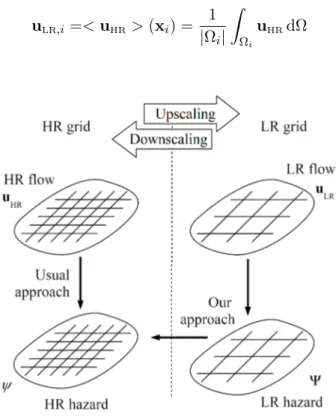
Figure 1: Workflow definition sketch. High Resolution (HR) hazard mapping (hazard indicator ψ) is usually obtained from CPU-intensive, HR flow simulations (flow variable uHR). The proposed downscaling
framework consists in obtaining HR hazard maps from CPU-efficient Low Resolution (LR), upscaled flow simulations (flow variable uLR and hazard indicator Ψ.)
2.3. Proposed downscaling framework
Downscaling is the reverse operation to upscaling, see Fig.1. As mentioned in subsection2.1, the usual approach to flood hazard assessment, represented by the downward arrow on the left-hand side of Fig. 1, consists in deriving the HR hazard indicator ψ, see (2), directly from the simulated HR flow variable uHR. The proposed downscaling framework consists of two steps :
(i) the LR hazard indicator Ψ is computed from the simulated LR flow uLR, as represented by the
downward arrow in the right-hand side of Fig.1, and (ii) the HR hazard indicator ψ is estimated from Ψ, as shown by the leftward arrow at the bottom of Fig. 1. As stated in the Introduction, statistical models are widely used to perform downscaling in the context of climate change studies. Although setting up the statistical models may require a certain amount of work, they are capable of providing fast and accurate estimates [2]. Two such statistical models adapted to this proposed downscaling framework for flood hazard assessment are described in section 3. To set up the statistical downscaling models for each considered flooding configuration, pairs of LR and HR flow simulations must be available from which LR and HR hazard indicators are derived. Within a given flooding configuration, the numerical values of the initial/boundary conditions are allowed to vary from one pair of simulations to the next, resulting in as many so-called flow scenarios. To ensure good performance of the statistical downscaling models,
a number of flow scenarios must be available representing sufficiently consistent space-time behaviours of the flow fields. Consistency is appreciated in terms of the broad behaviour of the flow (e.g. a positive wave heading to the left, a negative wave heading to the right, a set of frictionless simulations, etc.) It is expected that, for a given configuration, once the downscaling models have seen a representative number of flow scenarios, they can be applied to flow scenarios that were not necessarily seen before.
3. Statistical downscaling models
3.1. Cell-by-cell artificial neural network model
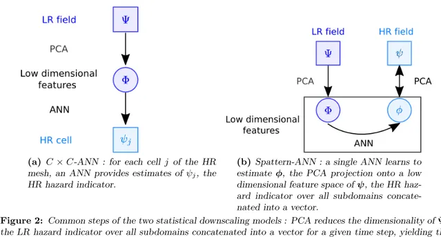
This downscaling model, called C × C-ANN for short, seeks to learn separately for each cell of the HR mesh a relationship between the HR hazard indicator values at that cell and information drawn from the LR hazard indicator over all subdomains. There are two main steps in this approach, represented by the arrows in Fig. 2a. The first step (top arrow in Fig. 2a) consists in summarizing the LR hazard indicator by features with fewer dimensions obtained by a Principal Component Analysis (PCA) [33]. The second step (bottom arrow in Fig. 2a) consists in learning a relationship between these low dimensional features and the HR hazard indicator values at a given cell of the HR mesh with an Artificial Neural Network (ANN) [7]. There are as many ANNs as cells where the HR hazard indicator needs to be estimated.
In the first step of C × C-ANN, the vector Ψk ∈ RD that concatenates the LR hazard
indicator over all subdomains at a given time tk, is summarized by Φk ∈Rdwith d < D, a low
dimensional feature representation, computed with PCA so as to minimize the L2 norm. The
low dimensional features Φk are in fact a projection of Ψk onto a linear subspace spanned by
the first d eigenvectors of the sample covariance matrix of Ψk. Let A ∈RD×Rd be such that
each column is one of the first d eigenvectors spanning the linear subspace, which are called principal components. Then, since A−1 = AT thanks to the orthogonality of the eigenvectors, PCA yields a decomposition of the form
Ψk = AΦk⇔ Φk= ATΨk. (6)
In the second step of C × C-ANN, the relationship between {Φk}k, the low dimensional
features summarizing the LR hazard indicator, and {ψj,k}k, the values of the HR hazard indicator
at mesh’s cell j is learned with an ANN. There are as many ANNs as cells j where ψjneeds to be
estimated. Each of these ANNs is implemented as shown in Fig.3awith a standard feed-forward architecture that includes one hidden layer plus a direct linear connection such that the case with no neuron in the hidden layer boils down to classical linear regression [7]. In what follows, the dependence on time, i.e. the subscript k, is dropped to unclutter the notation. In Fig. 3a, the input layer of the ANN consists of a special neuron permanently set to 1 to account for constants in the calculations and of the vector Φ = (Φ1, . . . , Φd) of d low dimensional features
extracted by PCA from the LR hazard indicator. The (d + 1) weight vector whidn connects the input layer to the nthneuron of the hidden layer, with 1 ≤ n ≤ Nh, through linear combinations
(a) C × C-ANN : for each cell j of the HR mesh, an ANN provides estimates of ψj, the
HR hazard indicator.
(b) Spattern-ANN : a single ANN learns to estimate φ, the PCA projection onto a low dimensional feature space of ψ, the HR haz-ard indicator over all subdomains concate-nated into a vector.
Figure 2: Common steps of the two statistical downscaling models : PCA reduces the dimensionality of Ψ, the LR hazard indicator over all subdomains concatenated into a vector for a given time step, yielding the lower dimensional vector Φ of features used as input vector for the ANN.
that are transformed non-linearly with a hyperbolic tangent as follows :
an(Φ; whidn ) = tanh d
X
i=1
whidn,iΦi+ wn,0hid
!
n = 1, . . . , Nh. (7)
In Fig. 3a, the output layer has a single neuron, ˆψj, that yields estimates of the HR hazard
indicator values at the HR cell j computed as :
ˆ ψj(Φ; w) = g Nh X n=1 woutn an(Φ; whidn ) | {z } non-linear + d X i=1 wlini Φi+ w0lin | {z } linear for a given j, (8)
where wout is a weight vector of length Nh connecting the hidden layer to the output neuron
through linear combinations, wlin is a weight vector of length (d + 1) that links directly the input layer to the output layer through linear combinations and g(·) = log(1 + exp(·)) serves to enforce positivity. The weight vector w of the ANN includes the weight vectors whidn with n = 1 up to Nh, the weight vector wout and the weight vector wlin.
For a given d, the dimension of the feature space computed by PCA, and a given Nh, the
number of neurons in the hidden layer, an ANN is trained separately for each cell j. The training procedure involves optimising the ANN’s weights w so as to minimise, over a training set made of pairs of the form {(Φk, ψj,k)}k, the following sum of squared errors :
Eloc(w; j) = 1 2
X
k
( ˆψj(Φk; w) − ψj,k)2. (9)
(a) C × C-ANN : separate ANN for each cell j with a single output neuron to estimate the HR hazard indicator value, see (7)-(8).
(b) Spattern-ANN : a single ANN whose out-put layer yields an estimate a low dimensional feature representation of the HR hazard indi-cator over all subdomains, see (7) and (11). Figure 3: Standard feed-forward artificial neural network architectures with one hidden layer plus a direct linear connection used in the two statistical downscaling models.
to efficiently compute the gradient [40]. To avoid local minimums, the optimisation is performed 10 times with random initial parameter values and the optimised parameters yielding the lowest error computed on the training set are retained. This optimisation strategy was assessed by monitoring closely several ANNs’ training.
As d and Nh are hyper-parameters, for each cell j, suitable values must be selected with a
validation procedure [7]. Indeed, the complexity level of C × C-ANN is directly related to the overall number of weights in the ANN which depends on d and Nh that control the size of the
input and the hidden layers respectively. The validation procedure works as follows. Several potential pairs of values are considered for the parameters. For each such pair of hyper-parameter values, the ANN’s weights are optimised on the training set. The performance of the ANN associated to each particular choice of hyper-parameter values is evaluated in terms of the sum of squared errors as in (9) but computed on a validation set, a data set distinct from the training set. The hyper-parameter values yielding the lowest validation error are retained. Different hyper-parameter values are likely to be selected for different cells when the complexity of the relationship learned by the ANNs differ.
3.2. PCA spatial pattern-based artificial neural network model
This second downscaling model, termed Spattern-ANN for short, seeks to learn a single relationship (as opposed to C × C-ANN that seeks to learn as many relationships as there are HR cells) between low dimensional features that summarize the HR hazard indicator and low dimensional features that summarize the LR hazard indicator. Spattern-ANN has four main steps, as shown by the arrows in Fig.2b. The first step (left top arrow in Fig.2b) is the same as C × C-ANN : the LR hazard indicator over all subdomains is summarized by low dimensional
features obtained by PCA. In the second step (right top downward arrow in Fig. 2b), the HR hazard indicator over all HR cells is also projected onto a low dimensional feature space with PCA. The third step (horizontal arrow in Fig. 2b) consists in learning a relationship between the low dimensional features of the LR hazard indicator and those of the HR hazard indicator with an ANN with a similar architecture as the one used in C × C-ANN, see Fig.3b. The fourth and last step (right top upward arrow in Fig. 2b) consists in reconstructing the HR hazard indicator over all HR cells from the low dimensional feature representation estimates provided by the ANN.
The second and fourth steps of Spattern-ANN also rely on the PCA decomposition this time applied to the HR hazard indicator instead of the LR hazard indicator. As for the LR hazard indicator, at a given time tk, let ψk∈RP, be the concatenation into a vector of the HR
hazard indicator over all HR cells, where P is the total number of cells of the HR mesh. Let B ∈ RP ×Rp, p < P be the matrix whose columns are the first p eigenvectors of the sample
covariance matrix of ψk. Then the PCA decomposition relates ψk to low dimensional features φk∈Rp as follows
ψk = Bφk⇔ φk= BTψk. (10)
The principal components, i.e. the eigenvectors contained in the columns of B, can be interpreted as spatial patterns. In Spattern-ANN, the HR hazard indicator is thus assumed to be a linear combination of these spatial patterns with the coefficients in the linear combination provided by the low dimensional features φk.
In the third step of Spattern-ANN, an ANN whose architecture is depicted in Fig.3b seeks to estimate {φk}k, the low dimensional features that serve to weight the spatial patterns in
order to reconstruct the HR hazard indicator, based on {Φk}k, the low dimensional features of
the LR hazard indicator. The ANN’s calculations at the hidden layer are as in (7) while at the output layer, the ANN has p neurons, see Fig. 3b, which perform the following calculations
ˆ φj(Φ; w) = Nh X n=1 wj,noutan(Φ; whid) | {z } non-linear + d X i=1
wj,ilinΦi+ wj,0lin
| {z }
linear
j = 1, . . . , p, (11)
where, as previously, the time index k is dropped and wout is now a Nh× p matrix instead of
a vector of length Nh. The size of the output layer and the absence of positivity constraints
on the output neurons are thus the only differences with the architecture of the ANNs used in C × C-ANN.
In the fourth step of Spattern-ANN, for any time tk, the estimated values of the HR hazard
indicator over all HR cells are given by
ˆ
ψ(Φk; w, B) = B ˆφ(Φk; w), (12)
Φk= ATΨk, see (6).
For a given d (size of the input layer), a given Nh (size of the hidden layer) and a given p
(size of the output layer), the ANN’s weigths w are optimized by minimising over a training set made of pairs {(Φk, φk)}k the following sum of squared errors :
Efea(w) = 1 2 p X j=1 X k ( ˆφj(Φk; w) − φj,k)2. (13)
The same optimisation strategy as in C × C-ANN is used : best optimised parameters out of 10 runs of back-propagated gradient descent algorithm with random initialisations.
In Spattern-ANN, three hyper-parameters control the number of weights in the ANN which is directly related to the complexity level of this approach : Nhand d, as in C ×C-ANN, together
with p, the dimension of the feature space of the HR hazard indicator, see (10). These hyper-parameters must also be selected with a validation procedure, as described in the C × C-ANN’s subsection. To take into account the impact of the choice of p, the dimension of the feature space of the HR hazard indicator, the sum of squared errors that measures the performance on the validation set is different than the one in (13) used for training :
Etot(w; B) = 1 2 P X j=1 X k ( ˆψj(Φk; w, B) − ψj,k)2. (14)
4. Low and high resolution simulated data sets
As mentioned in the Introduction section, a flooding configuration is defined as a given building geometry for which several flow scenarios, implemented with initial and/or boundary conditions, are considered. The HR data sets are obtained by solving the two-dimensional shallow water equations (1a)-(1c). The LR data sets are the perfect upscaled solution obtained by averaging the HR simulation over the subdomains as in equation (5).
4.1. Synthetic urban configurations
Five synthetic urban configurations are considered. They rely on a common layout consisting of a periodic array of length L made of building blocks (see Fig.4 and Table 1). The buildings are aligned along the x− and y−directions. The spatial period and building spacing in the X−direction (X = x, y) are denoted by LX and WX respectively. The computational domain
is discretised into a high resolution mesh with 62.5 cm × 62.5 cm square cells, for 46080 cells in total. The subdomains used to derive the perfectly upscaled solution uLR(see (5)) are delineated
by connecting the centroids of the building blocks (dashed line in Fig. 4). There are 20 such subdomains in total. Other options are available for the definition of the subdomains. For instance, they might be centred around the building blocks, or shifted by any distance in the x− and/or y−direction. Besides, the subdomains may include more than one x− and/or y− building period. The present choice is motivated by two main reasons: (i) the size Lx× Ly is the
resolution for the upscaled solution, (ii) defining the subdomains by connecting the centroids of the buildings is consistent with the meshing strategies required by a number of porosity-based shallow water models, such as the IP or DIP models [28,29,43].
Figure 4: Synthetic urban configurations : definition sketch for the geometry.
Parameter Meaning Numerical value
L Total domain length 1000 m
Lx x−Period length 50 m
Ly y−period length 50 m
Wx Width of N-S streets 10 m
Wy Width of E-W streets 10 m
Table 1: Synthetic urban configurations : geometric parameters.
The LR hazard indicator values over the 20 subdomains are used to constitute the vector Ψ ∈ R20 used as input in the two statistical downscaling models, see Fig. 2. However, owing to the high computational time required by C × C-ANN, the HR hazard indicator values are restricted to three subdomains located slightly after the beginning, at the middle and slightly before the end of the computational domain. The subdomains’ x -limits are [250 m, 300 m], [500 m, 550 m] and [750 m, 800 m]. These three subdomains are selected based on hydraulic considerations, more specifically flow gradients, that are representative of the whole domain. Each subdomain contains 2304 cells for a total of 6912 cells considering the three subdomains. Spattern-ANN, described in subsection 3.2, is applied on the full set of 6912 cells covering the three subdomains, i.e. ψ ∈R6912in Fig.2b. As C ×C-ANN, described in subsection3.1, requires to learn a separate relationship for each HR cell, the number of cells was reduced to 125 within each subdomain, for a total of 375 cells over the three subdomains, to keep the computation time within reasonable limits, i.e. {ψj}375j=1, in Fig. 2a. For each of the three subdomains, the
125 cells are selected as follows, see Fig.5. The subdomain is divided into 5 rectangular zones : one for the central crossroads and four for each of the branches departing from the intersection. Each of these five zones comprises 5 × 5 cells spread regularly so as to allow for a maximum coverage of the rectangular zone.
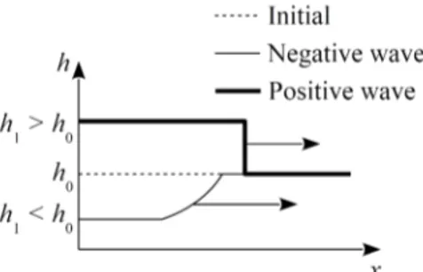
The first two synthetic configurations considered are 1D negative and positive waves without friction that are 1D Boundary Value Problems (BVPs). These configurations, identified as N-wave-nf and P-wave-nf respectively for short, are one of the simplest possible BVPs for layouts of this type. The frictionless propagation along the x−direction of a wave into still
-25 25
0 50
y (m)
x (m)
Figure 5: Synthetic urban configurations : locations of the 125 cells within a given subdomain. The origin of the coordinates are taken from the SW corner of the subdomain.
water is simulated (Fig.6). The bottom is flat, the water is initially at rest in the domain, with an initial depth h0. The water level is set instantaneously to a constant value h1 at the Western
boundary of the domain. In N-wave-nf, h1 < h0, which yields a negative wave (rarefaction
wave). In P-wave-nf, h1 > h0 and a positive wave (shock wave) appears. The LR solution uLR
is self-similar in the (x, t) domain [26,28,29].
Figure 6: Negative and positive wave configurations : initial and boundary condition definition sketch.
The next two synthetic configurations use the same geometry as N-wave-nf and P-wave-nf (Fig. 6) but with a non-zero bottom friction coefficient. These configurations, identified as N-wave-wf and P-wave-wf respectively, are cases study closer to real-world situations. As a consequence of the non-zero friction coefficient, the upscaled solution is no longer self-similar in the (x, t) space. Both the HR and LR simulations and their spatial gradients span a different range of hydraulic configurations from that of N-wave-nf and P-wave-nf.
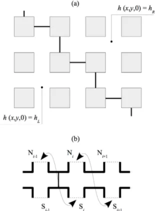
The last synthetic configuration, identified as Dam-break, is a 2D oblique urban dam break problem without friction. The dam break problem is a Riemann, Initial Value Problem (IVP) where the water is initially at rest and the water depth is piecewise constant, equal to hL and
hRrespectively on the left- and right-hand sides of a broken, divide line with average orientation
SE-NW (Fig. 7a). This results in an average flow field and wave propagation pattern oriented in the SW-NE direction. Since the flow is diagonal to the main street directions, fully meshing the domain involves as many block periods in both directions of space. This makes the mesh size and the subsequent computational effort prohibitive. The difficulty can be overcome [26]
by meshing only a single block period in the transverse direction (Fig.7b). The topology of the mesh is modified by connecting the Northern side of the ith lateral street (boundary segment Ni in the Figure) with the Southern side of the i + 1th lateral street (boundary segment Si+1
in Fig. 7b). While the upscaled solution of an urban dam break problem parallel to the main street axis is known to be self-similar in (x, t) [25, 28,26], self-similarity disappears when the propagation is oblique with respect to the street axes [26]. The Dam-break configuration includes both negative and positive wave phenomena.
Figure 7: 2D oblique dam break problem. Definition sketch : (a) building layout and IVP geometry in plan view (b) periodic model mesh for computational efficiency. Bold lines: impervious boundaries. Dashed lines: boundary segments with staggered connection scheme.
4.2. Field-scale test case
The field-scale test case considered was reported in [28] for the evaluation of a porosity-based, shallow water model. The frictionless propagation of a dike break flood wave into a neighbourhood of the Sacramento urban area is simulated. The test, which is referred to as Sacramento for short, is informative in many aspects: (i) the geometry is real, non-periodic, (ii) the upscaled hydraulic pattern is genuinely two-dimensional, and (iii) the HR flow field exhibits a strong polarisation along two preferential flow directions [28]. The dike breach is located on the left-hand side of the domain in Fig. 8. The Sacramento neighbourhood is discretised using a HR mesh made of 77 963 cells (average cell area 6.5 m2). For SPattern-ANN (subsection3.2), ψ ∈ R77 963 in Fig. 2b. C × C-ANN is restricted to an area containing 575 HR cells, i.e.
{ψj}575
j=1, in Fig. 2a. The LR mesh used for upscaling is much coarser, with 1682 subdomains
downscaling models, see Fig.2. These HR and LR meshes are used for the refined and porosity-based shallow water simulations reported in Guinot et al. [28]. Fig. 9 shows close-up views of the HR and LR meshes of the area where the 575 cells on which C × C-ANN is applied are located. 596400 597200 2036400 2037000 y (m) x (m)
Figure 8: Field-scale test (Sacramento) : Sacramento neighbourhood with the bold rectangle indicating the zooming areas in Fig.9.
596850 596925 2036600 2036700 y (m) x (m) Micro mesh 596850 596925 2036600 2036700 y (m) x (m) Macro mesh
Figure 9: Field-scale test (Sacramento) : area where the 575 cells (shown as red dots) on which C × C-ANN is applied are located. Top: HR mesh. Bottom: LR mesh.
4.3. Training, validation and test sets
In machine learning, the focus is on the evaluation of model performance on previously unseen data to assess the so-called generalisation capability [7]. The training set is used to optimise the parameters of each model, the validation set, distinct from the training set, serves to select the best hyper-parameter values while the test set, distinct from the training and validation sets, serves to compare the models with the selected hyper-parameter values. In the flood hazard framework, it is expected that statistical downscaling models, given a flooding configuration such as positive or negative waves, should be able to perform well at estimating the HR hazard indicator based on the LR hazard indicator for any flow scenarios. Therefore, the generalisation capability of a downscaling model may be measured in terms of performance, for a given configuration, at estimating flow scenarios that were not seen before. Thus, for each configuration, the training, validation and test sets are defined as pairs of HR and LR hazard indicators simulated for a number of flow scenarios.
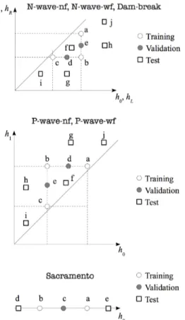
In Table2and 3, the flow scenarios labelled by a letter used to form the training, validation and test sets for the synthetic urban configurations and the field-scale test respectively are listed. Fig. 10 illustrates the principle of the training-validation-test sets’ design. The flow scenarios forming the training set are designed so as to span the space of BC and/or IC values. For the synthetic urban configurations, three flow scenarios, forming a right-angled triangle in the BC and/or IC space are needed since the space is two-dimensional. For the test-field case, only two flow scenarios are necessary as there is a single initial condition. The validation set is designed so as to contain flow scenarios such that only one of the BC and/or IC values is different from the values used in the training set but within their range. For the synthetic urban configuration, the validation set contains two flow scenarios taken as the midpoints of the two legs of the right-angled triangle. For the test-field case, the validation set consists of a single flow scenario defined by the IC value at the midpoint between the values forming the training set. The flow scenarios considered for the test set correspond to BC and/or IC values that extrapolate in different ways from the values seen for training and validation. For the synthetic urban configurations, five such flow scenarios are considered where as for the field-scale test only two possible flow scenarios are included in the test set.
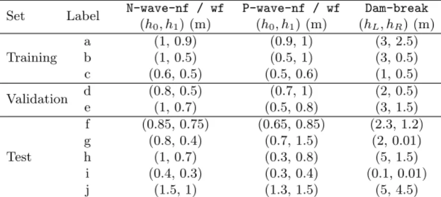
Set Label N-wave-nf / wf P-wave-nf / wf Dam-break (h0, h1) (m) (h0, h1) (m) (hL, hR) (m) Training a (1, 0.9) (0.9, 1) (3, 2.5) b (1, 0.5) (0.5, 1) (3, 0.5) c (0.6, 0.5) (0.5, 0.6) (1, 0.5) Validation d (0.8, 0.5) (0.7, 1) (2, 0.5) e (1, 0.7) (0.5, 0.8) (3, 1.5) Test f (0.85, 0.75) (0.65, 0.85) (2.3, 1.2) g (0.8, 0.4) (0.7, 1.5) (2, 0.01) h (1, 0.7) (0.3, 0.8) (5, 1.5) i (0.4, 0.3) (0.3, 0.4) (0.1, 0.01) j (1.5, 1) (1.3, 1.5) (5, 4.5)
Table 2: Flow scenarios defined in terms of BC and/or IC values used to form the training, validation and test sets for each of the synthetic urban configurations. The BC and/or IC values for the negative waves N-wave-nf / wf are not exact mirrors of those for positive waves P-wave-nf / wf in order to ensure the feasibility of boundary condition prescription.
Figure 10: Experiment plan definition sketch for each configuration : training, validation and test sets. Set Label h0 (m) Training a 6 m b 4.5 m Validation c 5.25 m Test d 3.5 m e 7 m
Table 3: Flow scenarios defined in terms of values of h0, the initial water depth in the channel, used to
form the training, validation and test sets for the field-scale test (Sacramento).
The sizes of the training, validation and test sets, compiled in Table 4, depend on the length of the simulation period T and the sampling time step which are set as follows. The sampling time step is 10 s in configurations N-wave-nf, N-wave-wf, P-wave-nf and P-wave-wf and 5 s for Dam-break and Sacramento. For each synthetic urban configuration, the length of the simulation period may change with the flow scenario so as to ensure that there is no wave reflection phenomena that would introduce completely different hydraulic behaviors and patterns. The negative wave configurations, N-wave-nf and N-wave-wf, have a duration of 400 s - 41 time steps - for all flow scenarios except for the “j” one which is set to 260 s - 27 time steps. P-wave-nf has a duration of 300 s - 31 time steps -in call cases except for the flow scenario labelled “g” that has a time span of 200 s 21 time steps. Pwavewf has a duration of 300 s -31 time steps - in all cases. Dam-break has a 100 s duration - 21 time steps - for all flow scenarios except the one labelled “j” that has a duration of 80 s - 17 time steps. The field scale simulation has a duration of 240 s - 49 time steps - except for the flow scenario labelled “d” which spans
480 s - 97 time steps - to allow the water to reach most areas.
Configuration Training Validation Test
N-wave-nf 123 82 191 N-wave-wf 123 82 191 P-wave-nf 93 62 145 P-wave-wf 93 62 155 Dam-break 63 42 101 Sacramento 98 49 146
Table 4: Training, validation and test set sizes for each configuration.
5. Evaluation and comparison of statistical downscaling models
5.1. Principal spatial patterns obtained from the training sets
Spattern-ANN, described in subsection 3.2, relies on the assumption that the HR hazard indicator can be decomposed into a linear combination of spatial patterns, see (10). These spatial patterns correspond to the eigenvectors contained in the matrix B of the PCA decomposition, termed principal components. The number of spatial patterns that may best reconstruct the HR hazard indicator, see (12), is selected on the validation set, see the following subsection5.2. A preliminary analysis of the spatial patterns uncovered by PCA is presented here in order to qualitatively assess their interpretability in terms of hydraulic behaviour. To this end, PCA is applied on the training set of each configuration, see Tables2-3, and the first six spatial patterns are illustrated for each of the two hazard indicators considered, i.e. the water depth and the norm of the unit discharge, see (2).
For the sake of conciseness, among the synthetic urban configurations, only the spatial patterns for Dam-break, which includes both negative and positive waves, are illustrated over the subdomain located in the middle of the computational domain, with x -limits [500 m, 550 m], as the other two subdomains have similar patterns. The oblique orientation of the spatial patterns is visible for both the water depth and the norm of the unit discharge, see Fig.11-12. In Fig.13
-14, the spatial patterns of the water depth and the norm of the unit discharge for Sacramento are shown. Although the spatial patterns of the norm of the unit discharge are sharper than those of the water depth, the general shape, with the propagation of the water from the breach in the dike located at the top left (see Fig. 8), is similar for both hazard indicators.
5.2. Hyper-parameter selected on the validation sets
Hyper-parameters are selected for each downscaling model following a data-driven procedure that relies on the performance evaluated on validation sets so as to estimate the generalisation capability. Several values are considered for each hyper-parameter so as to span the range of possibilities, starting from the lowest admissible value up to a value large enough to ensure that the selected value is not involuntarily bounded. The performance of each combination of values considered for each hyper-parameter is evaluated, i.e. the corresponding ANNs are trained, and the best combination, i.e. the one that yields the lowest error on the validation set, is retained. For the five synthetic urban configurations and the field-scale test, the hyper-parameters selected for the two downscaling models described in Section3and for the two hazard
(a) Spatial pattern 1 (b) Spatial pattern 2 (c) Spatial pattern 3
(d) Spatial pattern 4 (e) Spatial pattern 5 (f ) Spatial pattern 6
Figure 11: First six spatial patterns of the water depth for the Dam-break configuration obtained with PCA over the subdomain located in the middle of the computational domain. There is a common grey scale for all patterns with no units as the spatial patterns are eigenvectors that have unit norm.
(a) Spatial pattern 1 (b) Spatial pattern 2 (c) Spatial pattern 3
(d) Spatial pattern 4 (e) Spatial pattern 5 (f ) Spatial pattern 6
Figure 12: First six spatial patterns of the norm of the unit discharge for the Dam-break configuration obtained with PCA over the subdomain located in the middle of the computational domain. There is a common grey scale for all patterns with no units as the spatial patterns are eigenvectors that have unit norm.
(a) Spatial pattern 1 (b) Spatial pattern 2 (c) Spatial pattern 3
(d) Spatial pattern 4 (e) Spatial pattern 5 (f ) Spatial pattern 6
Figure 13: First six spatial patterns of the water depth for the Sacramento configuration obtained with PCA over the subdomain located in the middle of the computational domain. There is a common grey scale for all patterns with no units as the spatial patterns are eigenvectors that have unit norm.
(a) Spatial pattern 1 (b) Spatial pattern 2 (c) Spatial pattern 3
(d) Spatial pattern 4 (e) Spatial pattern 5 (f ) Spatial pattern 6
Figure 14: First six spatial patterns of the norm of the unit discharge for the Sacramento configuration obtained with PCA over the subdomain located in the middle of the computational domain. There is a common grey scale for all patterns with no units as the spatial patterns are eigenvectors that have unit norm.
indicators considered (water depth and norm of the unit discharge) are provided in Table5. For C × C-ANN, there are as many ANNs as HR cells (375 for the synthetic configurations and 575 for the field-test case, see Section4). Therefore, as many hyper-parameters as HR cells are selected. These are summarized by the median and the first and third quartiles in parentheses in Table5.
The values selected for d, the feature space dimension of the LR hazard indicator, may be very different for the two downscaling models. In particular, for Sacramento, low values (median of 3 for the two hazard indicators) are selected for C × C-ANN while high values (57 and 78 for water depth and unit discharge norm respectively) are chosen for Spattern-ANN. In contrast, for the unit discharge norm in the negative and positive wave configurations with or without friction, the values selected for d are similar. For Nh, the number of hidden units of the
ANN, C × C-ANN may select relatively high values for the positive wave configurations with or without friction for both hazard indicators. In contrast, in Spattern-ANN, Nh is almost always
zero, indicating that a linear relationship is sufficient as the complexity may be embedded in the feature space representations of the HR hazard indicator provided by PCA. Indeed, the values of p selected, the number of spatial patterns (or equivalently, the number of PCs) in Spattern-ANN, is much lower when the hazard indicator is in a configuration yielding smoother dynamics. This is the case for the water depth in the negative or positive wave configurations, with or without friction. In contrast, the water depth in the Dam-break and Sacramento configurations and the norm of the unit discharge, especially in the P-wave-nf / wf and Sacramento configurations, require higher numbers of spatial patterns. The only configuration in which the norm of the unit discharge requires less spatial patterns than the water depth is the Dam-break configuration.
Configuration
Water depth Norm of unit discharge
C × C-ANN Spattern-ANN C × C-ANN Spattern-ANN
d Nh d Nh p d Nh d Nh p N-wave-nf 20 (20, 20) 12 (4, 20) 8 0 5 10 (7, 12) 12 (1, 20) 12 0 20 N-wave-wf 20 (20, 20) 12 (4, 20) 8 0 5 10 (8, 13) 12 (2, 20) 10 0 10 P-wave-nf 19 (19, 20) 1 (0, 4) 19 0 5 19 (16, 19) 4 (2, 16) 19 0 40 P-wave-wf 16 (13 , 16) 1 (1, 2) 16 0 5 12 (12, 15) 2 (0, 4) 15 2 60 Dam-break 8 (8, 18) 0 (0, 1) 18 0 40 19 (14, 20) 1 (0, 8) 8 0 10 Sacramento 3 (2, 5) 2 (2, 2) 57 0 70 3 (3, 15) 1 (1, 2) 78 0 80
Table 5: Selected hyper-parameters for each configuration : d is the ANN input size (LR hazard indicator feature space dimension), Nhis the number of hidden neurons and p is the output size (HR hazard indicator
feature space dimension), see Fig.3. For C × C-ANN, the median is given with the first and third quartiles in parentheses computed over all the HR cells.
5.3. Relative errors computed on the test sets
The performance of C × C-ANN and Spattern-ANN is compared on test sets made of sev-eral flow scenarios, different than the ones that constitute the training and validation sets, see Tables2-3. Once again, performance evaluation on previously unseen data aims to estimate the generalisation capability of the models. The ANNs of the C × C-ANN - one per cell - and the ANN of Spattern-ANN with the hyper-parameters selected on the validation sets, see Table 5, are trained anew on a larger data set that merges together the training and validation sets. In
Tables 6 and 7, the performance is provided in terms of the following relative error computed on the test sets for all configurations and for both hazard indicators :
Rj,k = |ψj,k− ˆψj,k|
|ψj,k− Ψij,k|, (15)
for j, an element of the HR mesh, k, a simulation time step and ij, the subdomain to which cell
j belongs. Only time steps k such that |ψj,k− Ψij,k| is among the 5% largest values are kept in
the following analyses. This choice is made, on one hand, to avoid infinite or very large values of Rj,k as |Ψij,k − ψj,k| may be equal to zero or take on very small values and, on the other
hand, to focus on time steps that are more challenging owing to a greater variability within the subdomain. The relative error Rj,k from (15) can be interpreted as the estimation error
of the downscaling model relative to the error made when using LR hazard indicator values as surrogates for HR hazard indicator values. In particular, whenever Rj,k < 1, the downscaling
model provides more accurate estimates that the LR hazard indicator.
Table6concerns water depth downscaling and provides, for each configuration and each test set : in the second column, the minimum and maximum values taken by the simulated HR water depth field ; in the third column, ELR gives the 95% quantile of |ψj,k− Ψij,k|, the error of the
simulated LR water depth field ; in the last two columns, the median followed by the first and third quartiles in parentheses of Rj,kover time steps k such that |ψj,k−Ψij,k| > ELRfor each of the
two downscaling models. In Table6, it can be seen that C ×C-ANN outperforms Spattern-ANN, i.e. the inter-quartile interval of the relative error Rj,k is strictly smaller, for the two negative
wave configurations, N-wave-nf and N-wave-wf, over three test sets, labelled ”f”, ”g” and ”h”, out of five. However, for the two remaining test sets, labelled ”i” and ”j”, the relative error of C × C-ANN is greater than one, indicating that its absolute error is bigger than the absolute error of the LR hazard indicator. In contrast, the relative error of Spattern-ANN remains way below one for all test sets. For the two positive wave configurations, P-wave-nf and P-wave-wf, and for the Dam-break, the relative errors of both downscaling models is comparable and below one for the first three test sets labelled ”f”, ”g” and ”h”. For the last two test sets labelled ”i” and ”j”, the relative error of C × C-ANN reaches very high values whereas Spattern-ANN’s relative error remains low, although somewhat above one in some cases. For the field-scale test Sacramento, both downscaling models performed rather well although Spattern-ANN yielded slightly lower relative errors, especially for the first test set labelled ”d”.
Table 7 contains the same information as in Table 6 but concerns unit discharge norm downscaling. For this hazard indicator, the two downscaling models yielded, in most cases, a comparable performance. In particular, their relative error is low and bounded away from one. One notable exception is for the test set ”i” of Dam-break for which C × C-ANN yielded a very poor performance whereas Spattern-ANN performed relatively well, although with relative error values moderately above one. For Sacramento, Spattern-ANN provides a good performance on both test sets, with relative errors below one, whereas C × C-ANN is more challenged, especially for the first test set labelled ”d”.
Test (min ψ, max ψ) ELR C × C-ANN Spattern-ANN N-wave-nf f (0.75,0.85) 0.0054 0.024 (0.011,0.053) 0.12 (0.072,0.25) g (0.53,0.80) 0.013 0.007 (0.0032,0.015) 0.041 (0.017,0.069) h (0.7,1.0) 0.013 0.0034 (0.0015,0.01) 0.044 (0.022,0.079) i (0.31,0.40) 0.0048 1.6 (1.2,2.3) 0.041 (0.02,0.074) j (1.1,1.5) 0.023 2.1 (0.41,4.3) 0.041 (0.021,0.063) N-wave-wf f (0.76,0.85) 0.0043 0.029 (0.012,0.06) 0.19 (0.1,0.3) g (0.61,0.80) 0.0087 0.009 (0.0039,0.019) 0.064 (0.029,0.097) h (0.78,1.00) 0.0093 0.0051 (0.0019,0.013) 0.062 (0.03,0.11) i (0.35,0.40) 0.0029 1.8 (1.3,2.5) 0.1 (0.053,0.17) j (1.1,1.5) 0.018 1.1 (0.45,4) 0.058 (0.028,0.1) P-wave-nf f (0.65,0.90) 0.019 0.46 (0.2,0.91) 0.64 (0.34,1.2) g (0.49,1.65) 0.19 0.77 (0.33,1.2) 0.77 (0.64,0.89) h (0.19,0.81) 0.12 0.75 (0.44,1) 0.83 (0.69,0.91) i (0.30,0.43) 0.0091 3.6 (2.4,4.5) 0.53 (0.22,1.3) j (1.3,1.5) 0.015 8.4 (5.3,15) 0.63 (0.31,1.2) P-wave-wf f (0.65,0.84) 0.01 0.35 (0.17,0.68) 0.3 (0.092,0.67) g (0.62,1.42) 0.057 0.7 (0.35,1.3) 0.85 (0.75,1) h (0.30,0.66) 0.019 0.51 (0.21,1) 0.38 (0.23,0.69) i (0.30,0.36) 0.0028 8.8 (5.2,14) 0.36 (0.14,0.73) j (1.3,1.5) 0.013 8 (4.4,14) 0.44 (0.16,1) Dam-break f (1.2,2.3) 0.11 0.44 (0.19,0.91) 0.46 (0.22,0.68) g (0.0023,2.0000) 0.37 0.53 (0.33,0.68) 0.4 (0.3,0.51) h (1.4,5.0) 0.39 0.62 (0.33,0.95) 0.22 (0.097,0.51) i (0.0081,0.1000) 0.021 12 (11,14) 1.1 (0.43,1.5) j (4.5,5.0) 0.041 7.1 (3.9,12) 0.51 (0.34,0.95) Sacramento d (0.00,0.16) 0.018 1.7 (0.78,2.9) 0.36 (0.16,0.74) e (0.0,1.5) 0.22 0.13 (0.056,0.27) 0.056 (0.025,0.1)
Table 6: Water depth downscaling, from left to right : test set label, see Fig.10and Tables2-3; minimum and maximum value of the simulated HR water depth ; threshold value for |Ψij,k− ψj,k| determining the
time steps included in the analyses ; median (1st quartile, 3rd quartile) of the relative error Rj,k, see (15),
across all HR elements and all time steps such that |Ψij,k− ψj,k| > ELR for each statistical downscaling
model (see Section3). Bold font indicates when one of the downscaling models outperformed the other one (i.e. non-overlapping inter-quartile interval) while italic font indicates that the downscaling model performed better than a direct estimation with the LR field (i.e. values ≤ 1).
Test (min ψ, max ψ) ELR C × C-ANN Spattern-ANN N-wave-nf f (0.0,0.36) 0.18 0.0022 (0.00086,0.0054) 0.0023 (0.00074,0.0049) g (0.0,0.71) 0.31 0.0075 (0.0036,0.035) 0.0033 (0.00094,0.012) h (0.0,0.92) 0.43 0.0032 (0.00063,0.0061) 0.0016 (0.00048,0.0046) i (0.0,0.2) 0.08 0.044 (0.012,0.28) 0.017 (0.007,0.045) j (0.0,1.7) 0.73 0.03 (0.0066,0.35) 0.00088 (0.00028,0.0021) N-wave-wf f (0.0,0.3) 0.14 0.0085 (0.0034,0.021) 0.0037 (0.00094,0.012) g (0.00,0.43) 0.21 0.01 (0.0029,0.019) 0.0011 (0.00038,0.0031) h (0.00,0.61) 0.3 0.0044 (6e-04,0.011) 0.00064 (0.00021,0.0015) i (0.0,0.1) 0.047 0.029 (0.017,0.17) 0.0051 (0.002,0.016) j (0.0,1.3) 0.61 0.017 (0.0071,0.56) 0.0028 (0.0012,0.014) P-wave-nf f (0.0,1) 0.45 0.15 (0.059,0.26) 0.11 (0.066,0.16) g (0.0,5.8) 2.7 0.07 (0.024,0.96) 0.017 (0.0068,0.032) h (0.0,2.2) 1.1 0.03 (0.012,0.066) 0.0083 (0.0032,0.022) i (0.0,0.35) 0.14 0.084 (0.034,0.2) 0.066 (0.028,0.13) j (0.0,1.3) 0.59 0.088 (0.025,0.25) 0.073 (0.03,0.15) P-wave-wf f (0.0,0.72) 0.28 0.035 (0.013,0.086) 0.036 (0.015,0.072) g (0.0,3.4) 1.4 0.1 (0.026,0.38) 0.023 (0.0085,0.071) h (0.0,0.83) 0.36 0.05 (0.025,0.097) 0.021 (0.0071,0.047) i (0.0,0.16) 0.063 0.095 (0.014,0.29) 0.031 (0.0085,0.064) j (0.0,1.2) 0.49 0.049 (0.012,0.12) 0.039 (0.015,0.081) Dam-break f (0.0,3.5) 1.5 0.14 (0.11,0.16) 0.08 (0.037,0.12) g (0.0,3.6) 1.5 0.099 (0.04,0.17) 0.1 (0.043,0.21) h (0,12) 6.3 0.097 (0.051,0.14) 0.056 (0.028,0.12) i (0.0,0.046) 0.015 18 (12,22) 1.6 (0.46,2.6) j (0.0,3.1) 1.1 0.22 (0.1,0.43) 0.24 (0.099,0.41) Sacramento d (0.0,0.087) 0.015 1.4 (0.68,2.4) 0.35 (0.21,0.51) e (0.0,3.5) 0.78 0.18 (0.083,0.34) 0.033 (0.017,0.059)
Table 7: Unit discharge norm downscaling, from left to right : test set label, see Fig. 10 and Tables2
-3 ; minimum and maximum value of the simulated HR norm of the unit discharge ; threshold value for |Ψij,k− ψj,k| determining the time steps included in the analyses ; median (1
st
quartile, 3rdquartile) of the relative error Rj,k, see (15), across all HR elements and all time steps such that |Ψij,k− ψj,k| > ELR for
each statistical downscaling model (see Section3). Bold font indicates when one of the downscaling models outperformed the other one (i.e. non-overlapping inter-quartile interval) while italic font indicates that the downscaling model performed better than a direct estimation with the LR field (i.e. values ≤ 1).
6. Discussion
We proposed a downscaling framework (Subsection2.3and Fig.1) based on statistical mod-els to estimate HR hazard indicators from LR hazard indicators derived from upscaled flow simulations such as those obtained from porosity models. Two such statistical models are pro-posed in section3. Both rely on non-parametric, data-driven, approaches that are very flexible, since no strong parametric assumptions are made. Nevertheless, the training set must be suffi-ciently representative of the underlying structure that is being estimated in order to enable the non-parametric models to generalise well, i.e. to perform well on previously unseen data. In the operational phase, this downscaling framework offers a considerable speedup over running a HR simulation for each new flow scenario. For instance, for one flow scenario of N-wave-nf, 150 CPU s are needed to run the HR model. In comparison, running a LR porosity model and downscaling the results using the Spattern-ANN requires 7.5 × 10⁻³+ 2.22 × 10−2= 2.97 × 10⁻² CPU s. The speedup factor is thus slightly above 5000.
The first statistical downscaling model, named C ×C-ANN, is viewed as a reference approach as it relies on the same building blocks as conventional approaches to statistical downscaling that were applied in climate change studies, see Hewitson & Crane [31]. Furthermore, C × C-ANN is a univariate approach that does not attempt to capture the dependence structure of the HR hazard indicators. Indeed, downscaling is performed cell by cell, with an ANN dedicated to each cell of the HR mesh, see subsection 3.1 and Fig. 2a. A potential alternative to this reference approach would be to consider a single ANN that would be able to downscale all the cells of the mesh, one at a time, by including in its input specific information from each cell. For instance in Chadwick et al. [14], a climate variable simulated on a 25 km resolution grid by a Regional Climate Model (RCM) constrained by a GCM on a lower resolution grid of 1.89◦ is downscaled with a single ANN, one RCM cell at a time. Among the ANN input, there is information from the large scale variable at the four GCM grid cells surrounding the RCM grid cell of interest. By using information that changes with each RCM cell, the ANN is able to learn a relationship that can vary from cell to cell. Such an approach was considered initially in the shallow water models’ context but was put aside. Indeed, as the number of cells within each subdomain is very high, the question of which spatial information geographical coordinates not being sufficient -would be useful to help discriminate each cell has no straightforward answer.
The second statistical downscaling model, named Spattern-ANN, is capable of estimating very high dimensional fields such as the ones simulated by refined shallow water models, see subsection 3.2 and Fig. 2b. A key step of this downscaling model consists in decomposing the high dimensional HR hazard indicator into a linear combination of spatial patterns. PCA is often used to obtain spatial patterns from fields of climatic variables in order to infer weather types, i.e. recurring patterns that can be found, for instance, in large scale atmospheric circulation [53]. The weights of the linear combination of spatial patterns lie on a low linear subspace of the high dimensional HR hazard indicator called feature space. In the weather type approach mentioned above, clustering can be performed on the features, i.e. the linear weights obtained from PCA, to classify each time steps, e.g. days, into weather types. In contrast, in the proposed
Spattern-ANN model, these features are taken as the multivariate dependent variable in a regression model, a feed-forward neural network with a direct linear connection as in Fig. 3b. The aim of SPattern-ANN is to estimate the low dimensional features of the HR hazard indicators from the low dimensional features of the LR hazard indicators.
Several low- and high-resolution hydraulic simulations are used for the evaluation and the comparison of the statistical downscaling models, see section 4. In this paper, the perfect up-scaled solution is used, see (5), so as to evaluate the feasibility of such a downscaling framework when the upscaled flow fields are unbiased. This allows the error arising from scale change to be assessed, independently from the bias stemming from an inevitably inaccurate porosity model. Five synthetic urban flooding configurations are considered. These idealistic cases are interest-ing in that (i) they may appear as elementary components of more complex, real cases, (ii) their geometry is entirely under control, (iii) they allow the respective influences of the propagation and friction process to be assessed. One field-scale test is also included in the flooding config-urations. These pairs of HR and LR simulations serve (i) to set up the statistical downscaling models, i.e. to optimise their parameters and to select adequate hyper-parameter values with a training-validation procedure, and (ii) to evaluate their performance on flow scenarios, forming the test set, that were not used to set up the models. The underlying rationale is to assess the generalisation capability of the statistical downscaling models, i.e. their performance when estimating HR hazard indicator values for previously unseen flow scenarios.
A preliminary visual inspection of the spatial patterns obtained by PCA showed that these are interpretable according to each configuration and for the two hazard indicators considered -water depth and norm of the unit discharge (see Figs.11-12 and Figs.13-14, for the Dam-break and Sacramento configuration respectively). The selection of hyper-parameters on validation sets, see Table5, showed that, as was anticipated, Spattern-ANN needs more spatial patterns, i.e. a larger dimension of the feature space of PCA, to reconstruct the spatial field of more turbulent hazard indicators. With no hidden units selected in most cases for the ANN, Spattern-ANN is in fact a large dimensional multivariate linear regression. The complexity of Spattern-ANN is rather controlled by the aforementioned number of spatial patterns. The estimation of the model is carried out by combining three steps : (1) PCA of the LR hazard indicator, (2) PCA of the HR hazard indicator and (3) regression between the feature space of the low and high resolution fields. Despite being a linear model, the estimation could not be achieved with a single direct estimation step, as is the case with conventional linear regression, owing to the large dimension of the dependent variable. On the other hand, C × C-ANN requires decreasing hyper-parameter values, that are associated to a decreasing number of parameters in ANNs, for negative waves, positive waves, Dam-break and Sacramento, especially for water depth as the hazard indicator.
The relative error, see (15), used to evaluate the performance on the flow scenarios form-ing the test sets allows to directly assess the added value, in terms of absolute error, of the downscaling framework with respect to crude estimates provided by the LR hazard indicator. The following conclusions are drawn from Tables 6-7. For all five synthetic configurations, the flow scenarios labelled ”i” and ”j” proved to be more difficult most likely owing to the stronger
extrapolation in terms of BC and/or IC values with respect to the ones seen during training and validation, see Fig. 10 and Table 2. Comparing across synthetic configurations, regardless of the downscaling model used, negative wave configurations yield significantly smaller errors than positive wave configurations (compare N-wave- and P-wave- in Tables 6-7). Friction exerts a much milder influence on the performance of downscaling models than the wave pattern does (compare -nf and wf in the Tables). This was to be expected because negative wave configu-rations yield much smoother flow fields than positive waves. In most positive wave simulations, the moving shock spreads within one to two LR cells, inducing strong gradients and considerable variability in the HR flow. Such variability is very difficult to capture from the LR averaged variables. In contrast, negative waves often spread over several LR grid cells and the HR flow patterns are much less variable. In Dam-break, that includes both a negative and a positive wave, the error is clearly dominated by that of the moving shock. Besides, the waves propagate along the diagonal of the urban layout. This induces a larger HR flow variability than with the N-wave- and P-wave- configurations, where the waves propagate along the main axis of the urban layout. The question might then arise why the Sacramento configuration, that involves a positive wave, yields significantly smaller relative errors than the Dam-break configuration (com-pare, for instance, the performance of Spattern-ANN for Sacramento flow scenarios ”d”-”e” with Dam-break flow scenarios ”i”-”j”, that are all extrapolations). It must be noticed however that the wave in the Sacramento configuration propagates over a dry bottom. Therefore, the positive wave is essentially a rarefaction wave on the LR scale, not a shock. Shocks appear locally on the HR scale, but they are due to the local wave reflections against the building walls. They are not concentrated in the immediate neighbourhood of a moving bore as in the P-Wave and Dam-break configurations. As a conclusion, the smoothness of the flow, mainly driven by the wave propagation process, appears to be the predominant factor to downscaling accuracy.
7. Conclusion
The analyses carried out in this work showed that the proposed downscaling framework may yield fast and accurate estimates of the HR hazard indicators, either the water depth of the norm of the unit discharge, for a large number of flow scenarios for the five synthetic urban configurations and the field-scale test. In particular, the Spattern-ANN statistical downscaling model provided consistently good performance. Further work is needed to understand how to bring improvements to Spattern-ANN. An interesting avenue of research would be to investigate the representativeness of the spatial pattern basis. Does the training set contain informative enough data to uncover the spatial pattern basis ? In other words, does the training set include all the spatial patterns that are present in the validation and test sets ? Another avenue would be to consider techniques other than PCA to deduce the spatial patterns such as frames [18]. Besides, stochasticity could be introduced in the downscaling methods which would be helpful to account for uncertainties in the estimation. For C × C-ANN, it suffices to see the outputs of the ANN as the parameters of a given probability distribution [10,13]. For Spattern-ANN, the stochastic version of PCA could be implemented [7].
Other perspectives for this work are as follows. The hydraulic simulations reported involve a flat topography. The performance of the downscaling models in the case of a variable topography should be explored. In the case of a spatially variable bottom elevation, the free surface elevation is often smoother than the water depth. Whether the surface elevation is easier to downscale than the water depth should be assessed. In addition, imperfect upscaling should be tested as nonlocal effects are to be expected. However, the performance of the statistical downscaling models will not necessarily decrease as statistical strategies, termed ”bias correction” in the climate change context [2], might allow to circumvent the biases present in porosity model simulations. As mentioned in subsection2.1, the water depth and the norm of the unit discharge are not the only possible variables for flood hazard assessment. The possibility of downscaling additional variables such as the specific force per unit width and the hydraulic head should also be investigated. This might induce an increased level of complexity compared to the downscaling of the water depth and the unit discharge because the specific force and the hydraulic head are not conserved variables in the HR governing equations. Last, in some cases, only the maximum of a given flow variable within a given area might be needed for hazard assessment. In such cases, downscaling techniques developed within the theory of extreme values could be useful [5].
References
[1] Abt, S.R, Wittler, R.J, Taylor, A, & Love, DJ. 1989. Human Stability in a High Flood Hazard Zone. Water Resources Bulletin, 25, 881–890.
[2] Ayar, P. V., Vrac, M., Bastin, S., Carreau, J., D´equ´e, M., & Gallardo, C. 2016. Intercompar-ison of statistical and dynamical downscaling models under the EURO-and MED-CORDEX initiative framework: present climate evaluations. Climate Dynamics, 46(3-4), 1301–1329. [3] Bates, P.D. 2000. Development and testing of a sub-grid scale model for moving boundary
hydrodynamic problems in shallow water. Hydrol Processes, 14, 2073–2088.
[4] Bates, P.D., & De Roo, A.P.J. 2000. A simple raster-based model for flood inundation simulation. Journal of Hydrology, 236, 54–77.
[5] Bechler, A., Vrac, M., & Bel, L. 2015. A spatial hybrid approach for downscaling of extreme precipitation fields. Journal of Geophysical Research: Atmospheres, 120(10), 4534–4550. [6] Bernardini, G., Postacchii, M., Quagliarini, E., Brocchini, M., Cianca, C., & D’Orazio. 2017.
A preliminary combined simulation tool for the risk assessment of pedestrians’ flood-induced evacuation. Environmental Modelling & Software, 96, 14–29.
[7] Bishop, C. M. 2011. Pattern Recognition and Machine Learning. Information Science and Statistics. Springer.
[8] Blanco-Vogt, A., & Schanze, J. 2014. Assessment of the physical flood susceptibility of buildings on a large scale – conceptual and methodological frameworks. Nat. Hazards Earth Syst. Sci., 14, 2105–2117.
[9] Bruwier, M., Archambeau, P., Erpicum, S., Pirotton, M., & Dewals, B. 2017. Shallow-water models with anisotropic porosity and merging for flood modelling on Cartesian grids. Journal of Hydrology, 554, 693–709.
[10] Cannon, A. J. 2012. Neural networks for probabilistic environmental prediction: Condi-tional Density Estimation Network Creation and Evaluation (CaDENCE) in R. Computers & Geosciences, 41, 126–135.
[11] Cannon, A. J. 2018. Multivariate quantile mapping bias correction: an N-dimensional probability density function transform for climate model simulations of multiple variables. Climate dynamics, 50(1-2), 31–49.
[12] Cannon, Alex J, & Whitfield, Paul H. 2002. Downscaling recent streamflow conditions in British Columbia, Canada using ensemble neural network models. Journal of Hydrology, 259(1-4), 136–151.
[13] Carreau, J., & Vrac, M. 2011. Stochastic downscaling of precipitation with neural network conditional mixture models. Water Resources Research, 47(10).
[14] Chadwick, R., Coppola, E., & Giorgi, F. 2011. An artificial neural network technique for downscaling GCM outputs to RCM spatial scale. Nonlinear Processes in Geophysics, 18(6). [15] Chanson, H., & Brown, R. 2015. Discussion on “New criterion for the stability of a human