Appendix E
BACKGROUND TO STRAIN GAUGE AND EXTENSOMETER
CALIBRATIONS
Table of contents
1. Strain Gauge Calibrations... 1
1.1 Variation of strain gauge factor with location around caisson ... 1
1.2 Previous estimates of calibration factors ... 2
1.3 Detailed explanation of strain gauge calibration factors in Appendix F ... 4
1.4 Estimates of calibration factors for the present study... 9
2. Extensometer Calibrations... 11
2.1 Previous estimates of extensometer calibration factors... 11
2.2 Detailed explanation of extensometer calibration factors in Appendix F ... 12
2.3 Synopsis of extensometer calibrations from Appendix F... 15
2.4 Sandwell report on extensometer calibration ... 15
2.5 Influence of load distribution across the centre face on extensometer response.18 List of Figures Figure 1 Strain gauge calibration factors on tributary width of 2.44 m for east and north faces of Molikpaq. Values fitted with a curve are those given in Table 3. Values plotted as points only are the calibration factors calculated for events on February 17, March 25, April 12 and May 12, 1986 (Spencer et al., 1989)... 3
Figure 2 Normalized strain gauge factors (in tonnes/m/μstrain) for east and north faces of Molikpaq (Jefferies and Spencer, 1989) ... 4
Figure 3 Calibration Event “5”: Load on MEDOF panel group N2, with and without the contribution of lower panel 1010, and strain gauge N2 ... 6
Figure 4 Calibration Event “5”: Calibration of strain gauge N2 against MEDOF panel group load (including lower panel 1010)... 7
Figure 5 Calibration Event “5x”: Calibration of strain gauge N2 against MEDOF panel group load (without lower panel 1010) ... 7
Figure 6 Calibration Event “5J”: Calibration of strain gauge N2 against MEDOF panel group load (including lower panel 1010)... 8
Figure 7 Calibration Event “5Jx”: Calibration of strain gauge N2 against MEDOF panel group load (without lower panel 1010) ... 8
Figure 8 Strain gauge and MEDOF results for FAST file F604121101... 9
Figure 9 MEDOF panel and strain gauge measurements for location E2 (note that sign of strain gauge result has been reversed for plot) ... 10
Figure 10 Cross-plot of strain gauge and MEDOF panel measurements for the time period 11:51 to 12:00 on April 12, 1986 ... 10
Figure 11 Non-linear horizontal displacement of the structure in response to ice loading (from Sladen and Hayley, 1988) ... 12
Figure 12 MEDOF Panel column loads and N-S extensometer for March 25, calibration Event “1” ... 13
Figure 13 Pot of North face load versus N-S extensometer deformation for Calibration Event “1” ... 13
Figure 14 MEDOF Panel column loads and N-S extensometer for April 12, Calibration Event “9” ... 14
Figure 15 Plot of East face load versus E-W extensometer deformation for
Calibration Event “9” ... 14
Figure 16 Horizontal movements of North and South faces of caisson for March 25 loading event ... 17
Figure 17 Deformation of caisson for March 25 loading event, comparison of two FEA programs ... 17
Figure 18 Time series of MEDOF column loads on morning of March 25 ... 18
Figure 19 Profiles of column loads for March 25 morning event ... 19
Figure 20 Loading cases for beam deflections ... 20
List of Tables Table 1 Strain gauge calibration factors used in DynaMAC (Rogers et al, 1998)... 2
Table 2 Strain gauge calibration factors for various heights of applied load on the North face (Smyth and Spencer, 1987) ... 2
Table 3 Strain gauge calibration factors for various ice thicknesses (Spencer et al, 1989)... 3
Table 4 Strain gauge calibration factors determined for this project (kN/µstrain for width of 2.44 m) ... 11
Table 5 Extensometer calibration factors determined for this project (MN/mm) for face loads ... 15
1. STRAIN GAUGE CALIBRATIONS
1.1 Variation of strain gauge factor with location around caisson
The strain gauge response depends on the stiffness of the bulkhead to which it is attached. The calibration factors vary by up to 30% depending upon the location of the strain gauge. Differences in calibration factors can be attributed to local variations in stress patterns in the main bulkheads, such as the proximity to watertight bulkheads, corners or pump rooms. It is assumed that the lower response of the strain gauges at these types of
locations is a result of more of the applied load being transmitted through the stiffer parts of the structure (Rogers et al, 1991). A lower strain gauge response results in a higher calibration factor, since the factor is the load (in kN) per μstrain of strain gauge response. For example, bulkheads N2, E2, S2 and W2 were all adjacent to full watertight bulkheads and have a higher strain gauge factor than gauges at other locations.
As a further check on the sensitivities of various bulkheads, a comparison was made between the SG09 gauge and the ‘C-10’ gauge, which is located at lower positions on the same bulkhead. If the variation in the response of the SG09 gauges is indeed caused by load sharing to adjacent steel work, we would expect to see a similar pattern in the ‘C-10’ and SG09 gauge responses. However, if the bulkhead sensitivities were related to stress concentrations around gauges or gauge placement inaccuracies, then we would not expect to see the same pattern in response for the different gauges. Rogers et al (1991) found that there is a directly proportional relationship between the ‘C-10’ and SG09 gauges (within an accuracy of ±20%), indicating that the bulkhead sensitivity is largely influenced by load sharing to adjacent structures.
Average calibration factors calculated by Rogers et al (1998) for each SG09 strain gauge are shown in Table 1. Data were taken for a number of loading events during the winter. The values in Table 1 are best estimates based on direct calibration by ice loading,
supplemented by calibration factors determined by finite element calculations and
simulation of loading by deballasting. During the deballasting procedure, ice loading was simulated by pumping water out of caisson ballast tanks in order to generate a known exterior load due to water pressure on the Molikpaq.
Table 1 Strain gauge calibration factors used in DynaMAC (Rogers et al, 1998)
1.2 Previous estimates of calibration factors
Because of the importance of the calibration factors for converting strain to load, earlier work was also reviewed. The starting point was the Smyth and Spencer (1987) review of measurement techniques. They applied a finite element analysis of the bulkhead structure to check the calibration of the SG09 gauges for determining local ice loads. A uniformly distributed horizontal load of 100 MN was applied to the North face at 4 different heights above the base of the caisson, and strains were computed as shown in Table 2. Resistance was provided by the sand core.
Table 2 Strain gauge calibration factors for various heights of applied load on the North face (Smyth and Spencer, 1987)
Case
Height of applied load, from base of
caisson (m) Approximate corresponding ice thickness (m) Stress (MPa) Strain (µstrain) Calibration factor (kN/µstrain) 1 18.4 2.2 59.4 283 14.4 2 17.4 4.2 66.5 317 12.8 3 16.4 6.2 57.3 273 14.9 4 15.4 8.2 42.9 204 19.9
Based on the finite element analysis and an evaluation of loading events when the MEDOF panels were responding well, Spencer et al. (1989) put forward their following best estimates of the strain gauge calibration factors as shown in Table 3. These factors show a strong dependence on ice thickness but follow a similar relative pattern to those of Table 1 for distribution across the faces; that is N2 and E2 have higher calibration factors than their neighbouring areas, N1 and N3, and E1 and E3, respectively.
Table 3 Strain gauge calibration factors for various ice thicknesses (Spencer et al, 1989) (kN/µstrain) over 2.44 m Ice Thickness (m) N1 N2 N3 E1 E2 E3 1 29.9 37.2 28.2 23.3 29.0 22.0 2 15.2 18.9 14.3 27.4 34.1 25.8 3 17.2 21.5 16.3 29.9 37.2 28.2 4 19.0 23.7 17.9 31.7 39.5 29.9 5 20.8 25.9 19.6 33.5 41.7 31.6 6 24.8 30.9 23.4 35.5 44.2 33.5
The calibration factors from Table 3 have been plotted as the curves in Figure 1 to make clearer the influence of ice thickness. Also plotted on this figure are calibration factors that were determined by Spencer et al (1989) for ice 0.8 m thick on February 17, 1986, 2.75 m thick on March 25, 1986, 2.5 m thick on April 12 and 1.8 m thick on May 12, 1986. It can be seen that for ice thickness 1.8 m to 2.75 m the agreement between the best estimates and factors determined from analysis of measured data is good.
0 5 10 15 20 25 30 35 40 45 0 1 2 3 4 5 6 7 Ice Thickness (m) S G F a ct or ( k N // µ str a in) N1 N2 N3 E1 E2 E3 N1 N2 N3 E2 E3 N1 N2 N3 E1 E2 E3
Figure 1 Strain gauge calibration factors on tributary width of 2.44 m for east and north faces of Molikpaq. Values fitted with a curve are those given in Table 3. Values plotted as points only are the calibration factors calculated for events on February 17, March 25, April 12 and May 12, 1986 (Spencer et al., 1989).
Jefferies and Spencer (1989) also make a presentation of the influence of ice thickness on a normalized calibration factor; see Figure 2. This figure is a simplified form of Figure 1, just giving a single curve for all areas on the North and East faces. There is considerable evidence that ice thickness is too important a factor to ignore in analysis. For example, during the morning of April 12 the ice impacting the east face was over 6 m thick at some points, which is higher than the average value used to calculate the strain gauge factors in Table 1. Using 6 m as the ice thickness, the maximum extrapolated calibration factors on the east face could be as much as 20% to 50% higher than the calibrations factors of Table 1.
Figure 2 Normalized strain gauge factors (in tonnes/m/μstrain) for east and north faces of Molikpaq (Jefferies and Spencer, 1989)
1.3 Detailed explanation of strain gauge calibration factors in Appendix F
A table with the results of extensometer and strain gauge calibrations is given in Appendix F. There are two parts to Appendix F, one in which the lower panels of N2 (1010) and E2 (1030) are either included (with pseudopanels) or not (without pseudopanels). In the other part, loads from pseudo panels are distributed to each MEDOF panel group as discussed in the main body of the Final Report. This table includes analysis of entire day files, entire fast files, as well as segments of fast files (colour coded as explained in the legend at the bottom of the table). Ten full files, and various segments of these files, are analysed from March 25, April 12, May 12, and May 22, 1986. The east, north and northeast faces were instrumented with MEDOF panels, but the northeast panels were non-operational for most of the winter. Therefore either the east, north, or both faces may be analysed for
calibration depending on which face(s) were loaded during the event. For example, Event “9” on April 12 involved ice loading on the east, southeast and south faces. Therefore the calibration was done for the east face.
Two DAY files are analysed, one for March 25 and one for May 22, 1986. It is important to point out that the calibration results from DAY files may be inaccurate since the DAY files measured only the average, maximum and minimum values for each channel for
every 5 minute interval (see Section 3 of the main Final Report). These values may occur at any time within the 5-minute interval. For the analysis in Appendix F, the maximum values are used to calibrate the strain gauges or extensometers against the MEDOF panels. The peak values for the different instruments may not necessarily occur at the same time, resulting in errors if used for calibration. Therefore the DAY files are analysed out of interest, but the results are considered to be less accurate than those from FAST files. No DAY file results were included in any of the averages.
FAST files are generally recorded at 1 Hz as explained in Section 3 of the main Final Report. For the fast files, calibration factors were calculated for various segments of time in addition to the calibration factor for the entire file.
In order to calibrate other instruments against the MEDOF panels, it is important that we have the correct MEDOF panel load. For ice up to 3 m thick, the MEDOF panels cover a sufficient area vertically to capture the loads generated by the entire thickness of the ice. For thicker ice, there is a concern that the MEDOF panels groups without a lower panel (E1, E3, N1 and N3) will not register the entire load as discussed in Section 4 of the main Final Report. The centre panel groups, N2 and E2, each have one additional lower panel. The effect of the lower panel on calibration results was studied using events on April 12 and May 22, 1986, during which the ice was thicker than 3 m. The results are presented in the Calibration Table in Appendix F. As an example the analysis of FAST file
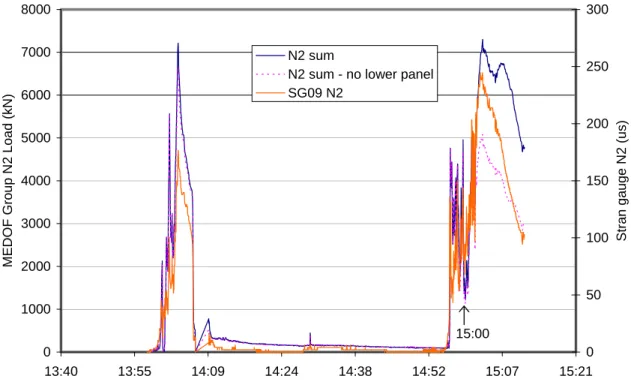
F605221301 is presented. This file covers the period of 13:57:40 to 15:11:32 on May 22, 1986. During this time, the observed ice thickness was 3 to 4 m, with ridges up to 2 m high. The ice was moving towards the southwest and ice loading occurred on the north, northeast and east faces. The following analysis is for ice loading on the north face. Figure 3 shows the total load on MEDOF panel group N2, with and without the
contribution of the lower panel. It is noted that the lower panel contributes very little to the total load for the period of 13:57 to 15:00. After this time, the lower panel makes a significant contribution to the load (maximum load of 7270 kN vs. 5030 kN without the lower panel). Also shown in Figure 3, for comparative purposes, is the output of stain gauge N2. The N23 SG09 output follows the general form of the MEDOF N2 panel group load.
MEDOF N2 group 0 1000 2000 3000 4000 5000 6000 7000 8000 13:40 13:55 14:09 14:24 14:38 14:52 15:07 15:21 MEDOF Group N2 Load (kN) 0 50 100 150 200 250 300 Stran ga uge N2 (us) N2 sum
N2 sum - no lower panel SG09 N2
15:00
Figure 3 Calibration Event “5”: Load on MEDOF panel group N2, with and without the contribution of lower panel 1010, and strain gauge N2
The calibration of the SG09 strain gauge N2 against the MEDOF panel group N2
(including the contribution of the lower panel), is shown in Figure 4. This analysis is for the entire FAST file and corresponds to Calibration Event “5”, May 22, in Appendix F. The calibration of the same strain gauge against the MEDOF data (NOT including the contribution of the lower panel) is shown in Figure 5. This corresponds to Event “5x” in Appendix F. The calibration factor for Event “5” is 32.55 kN/µstrain, which is 45% greater than that for Event “5x”. This indicates that the load from the lower panel has a significant effect on the calibration of the strain gauges for this event.
y = -32.55x + 352.68 R2 = 0.9394 0 1000 2000 3000 4000 5000 6000 7000 8000 9000 -300 -250 -200 -150 -100 -50 0 50 SG09 N2 (microstrain) M E D O F pa ne l gr ou p N 2 l o ad ( k N
Figure 4 Calibration Event “5”: Calibration of strain gauge N2 against MEDOF panel group load (including lower panel 1010)
y = -22.49x + 322.71 R2 = 0.9156 0 1000 2000 3000 4000 5000 6000 7000 -300 -250 -200 -150 -100 -50 0 50 SG09 N2 (microstrain) M E D O F pa ne l gr ou p N 2 l o ad ( k N
Figure 5 Calibration Event “5x”: Calibration of strain gauge N2 against MEDOF panel group load (without lower panel 1010)
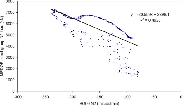
Next the time period for which the lower MEDOF panel makes the greatest contribution to the total load – that is, from 15:00 to the end of the file (15:11:32), “Calibration Event 5J” is examined. For calibration of strain gauge N2 against the MEDOF panel group including the lower panel (Event “5J” in Appendix F), the calibration factor is 20.56 kN/µstrain. As shown in Figure 6, the correlation between the MEDOF panels and strain gauges is very low with an R2 value of 0.49. When the lower MEDOF panel is omitted from the analysis (Figure 7), the calibration factor is reduced to 15.35 kN/µstrain. In this case the
value is unreasonably low. However overall, as shown in the Calibration Table in Appendix F, the correlation between MEDOF and strain gauge loads is usually better when the lower panel is included.
y = -20.559x + 2398.1 R2 = 0.4926 0 1000 2000 3000 4000 5000 6000 7000 8000 -300 -250 -200 -150 -100 -50 0 SG09 N2 (microstrain) M E D O F pan el grou p N2 lo ad (k N )
Figure 6 Calibration Event “5J”: Calibration of strain gauge N2 against MEDOF panel group load (including lower panel 1010)
y = -15.353x + 1323.2 R2 = 0.7488 0 1000 2000 3000 4000 5000 6000 -300 -250 -200 -150 -100 -50 0 SG09 N2 (microstrain) MED O F pan el g roup N 2 loa d ( k N )
Figure 7 Calibration Event “5Jx”: Calibration of strain gauge N2 against MEDOF panel group load (without lower panel 1010)
1.4 Estimates of calibration factors for the present study
Because strain gauge calibration is such a critical issue we carried out our own
independent analysis of calibration factors. A detailed table with ice information and strain gauge calibration factors for 11 files, as well as for individual segments of many files, is given in Appendix F. Note that the “Calibration analysis Event numbers” are different from the event numbers in Appendix A.
April 12, 1986 is one day for which several individual segments of files were analysed. The FAST file F604121101 is presented here as an example (Event “9” in Appendix F). The entire time series with strain gauge and MEDOF results is shown in Figure 8. The MEDOF panel load is the arithmetic sum of the five panels in group E2.
-2000 0 2000 4000 6000 8000 10000 12000 14000 04/12/86 11:02 04/12/86 11:16 04/12/86 11:31 04/12/86 11:45 04/12/86 12:00 04/12/86 12:14 04/12/86 12:28 04/12/86 12:43 MEDOF panel group load (k N) -50 0 50 100 150 200 250 300 350 St rain gauge result (mic rost rain) MEDOF Group E2 SG09 E2
Figure 8 Strain gauge and MEDOF results for FAST file F604121101
Figure 9 shows one time segment from this file for which strain gauge loads were
compared to the MEDOF panel results. A cross-plot of the MEDOF panel load and strain gauge results is shown in Figure 10. This time period corresponds to Event “9B” in the Calibration Table in Appendix F (a detailed explanation of the table is given in Section 1.3 of this Appendix). The MEDOF panel load is calculated using all five available panels but no pseudopanel (for this time period, there was no loading on the lower panel, so including a pseudopanel would not affect the result). The slope of the regression line represents the calibration factor for this segment of time. In this case the slope is approximately 36 kN/μstrain, which is greater than the average calibration factor of -30 kN/μstrain for SG09 E2 given in Table 1. These calibration factors were said to have an accuracy of ±30%, so the calibration factor determined from the measurement record on April 12 (Figure 9 and Figure 10) is within this range. Comparison of strain gauge and
from -20 to -42 kN/μstrain. The relatively high calibration factors obtained for the ice loading on April 12, 1986 are likely due to the thick ice for that day (at least 4 to 6 m).
0 2000 4000 6000 8000 10000 12000 14000 04/12/86 11:51 04/12/86 11:52 04/12/86 11:54 04/12/86 11:55 04/12/86 11:57 04/12/86 11:58 04/12/86 12:00 MED O F pan el gro up lo ad (k N) 0 50 100 150 200 250 300 350 St rain g aug e res u lt (mic rost rain) MEDOF Group E2 SG09 E2
Figure 9 MEDOF panel and strain gauge measurements for location E2 (note that sign of strain gauge result has been reversed for plot)
y = -35.854x - 183.35 R2 = 0.9766 -2000 0 2000 4000 6000 8000 10000 12000 14000 -350 -300 -250 -200 -150 -100 -50 0 SG09 E2 (microstrain) MED O F pane l gro up lo ad ( k N )
Figure 10 Cross-plot of strain gauge and MEDOF panel measurements for the time period 11:51 to 12:00 on April 12, 1986
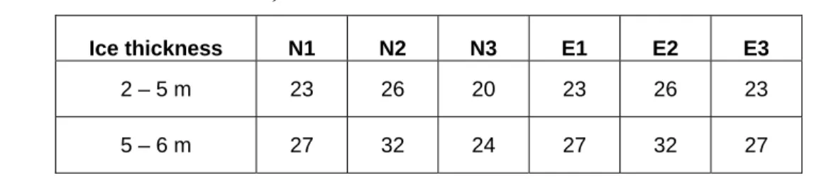
The results of the analysis in Appendix F have been divided such that an average
calibration factor is calculated for time series with ice thickness of 2 to 5 m, and 5 to 6 m. Based on these results, best estimates of the calibration factors are determined as shown in Table 5.
Table 4 Strain gauge calibration factors determined for this project (kN/µstrain for width of 2.44 m) Ice thickness N1 N2 N3 E1 E2 E3 2 – 5 m 23 26 20 23 26 23 5 – 6 m 27 32 24 27 32 27
2. EXTENSOMETER CALIBRATIONS
2.1 Previous estimates of extensometer calibration factors
In several reports to date, a factor of 6 MN/mm has been used to relate the extensometer measurements to a global load (Rogers et al, 1998, Bercha et al, 1994, and Rogers et al, 1991). Rogers et al (1991) based their value for global stiffness on data from events on March 25, 1986, and late in the day on May 12, 1986. For the event in March, a face load of 120 MN on the North face caused a displacement of 0.020 m, corresponding to a stiffness of 6.00 MN/mm. For the May event, a face load of 220 MN caused a displacement of 0.0435 m, corresponding to a stiffness of 5.05 MN/mm.
The Phase 1A report on Molikpaq performance at Amauligak I-65 (Gulf Canada Ltd., 1987b) estimated the calibration factor to be roughly 2000 tonnes (19.6 MN) per 1 mm deflection. This calibration factor actually represents the deflection of the face
perpendicular to the direction of the load. For this report, only the calibration factor for
deflection in the same direction as the load will be used.
As part of Gulf Canada’s study of dynamic ice/structure interaction (Rogers et al, 1991), Sandwell Inc. was contracted to perform a finite element analysis of the Molikpaq. The model was 3-dimensional and included the structural properties of the caisson and the sand core, and their interaction. The one limitation of the model was that only linear behaviour for the sand core could be represented. Simulations with the Gulf Canada provided values of the sand core stiffness resulted in load distortion ratios in the range of 2.0 to 4.2 MN/mm, which is approximately half the observed estimate of 6 MN/mm. Another finite element analysis, conducted earlier by GEOTECHnical Resources Ltd (Smyth and Spencer, 1987), examined the deflection caused by two loading cases. In the first case a 100 MN uniformly distributed load was applied to the North face of the structure, resulting in 8.2 mm net deflection of the face, or a calibration factor of 12.2 MN/mm. In the second case a 1 MN point load was applied, which resulted in 0.193 mm deflection or a calibration factor of 5.2 MN/mm. This shows that the nature of the load distribution on the face is important in determining the factor for converting diametral change to face load. They also modified the model to include base friction and calculated a deflection of 12.2 mm of the loaded face and no movement of the opposite unloaded face. For this more realistic boundary condition the calibration factor was 8.2 MN/mm. The previously discussed factors for converting extensometer data to face loads have all
performance have presented a non-linear response of the structure based on the
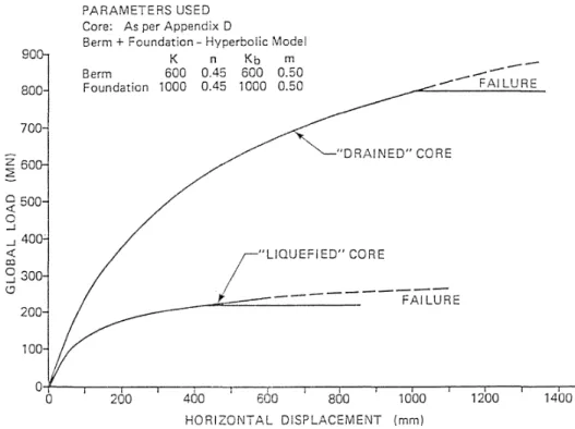
geotechnical properties of the sand core. Sladen and Hayley (1988) presented a non-linear horizontal displacement of the structure in response to ice loading as shown in Figure 11. They present results for “drained” and “liquefied” sand cores indicating that the response is non-linear in either case and that “strain-softening” behaviour is demonstrated. The initial slope for displacements up to 50 mm was about 3 MN/mm for the “drained” case. An independent analysis by Altaee and Fellenius (1994) derived response of the sand core from an assessment of the geotechnical properties of sand core. They used a plane-strain representation of the structure and also found a non-linear response, but with an initial stiffness of 6 MN/mm. In both cases the steel caisson was treated as a rigid body, but the caisson ring stiffness was not included in the analysis, so behaviour was controlled by the sand properties only. The Sandwell report in Rogers et al. (1991) treated both the caisson and the sand core and berm and their combined response to ice loading. Unfortunately the FE program used, COSMOS/M, became unstable when modelling non-linear sand core behaviour. It could be expected that the overall behaviour of caisson ring and core was non-linear, but no information is available to quantify any non-linearity.
Figure 11 Non-linear horizontal displacement of the structure in response to ice loading (from Sladen and Hayley, 1988)
2.2 Detailed explanation of extensometer calibration factors in Appendix F
A table with the results of extensometer calibrations is given in Appendix F. As already discussed in Section 1.2, means of dealing with the lower MEDOF panels are presented. This table includes analysis of entire day files, entire fast files, as well as segments of fast files (colour coded as explained in the legend at the bottom of the table). Ten full files, and various segments of these files, are analysed from March 25, April 12, May 12, and May 22, 1986. As an example, a time series plot of Calibration Event “1” in March 25 is plotted in Figure 12. It can be seen that the MEDOF column loads and the deformation across the North and South faces given by the N and S extensometers compare closely..
March 25 am - F603250801 0 500 1000 1500 2000 2500 3000 3500 8:24:00 8:38:24 8:52:48 9:07:12 9:21:36 9:36:00 9:50:24 time Med o f C o lu mns ( k N ) -14 -12 -10 -8 -6 -4 -2 0 N -S E x tens omet e r (mm) N1a N1b N2a N2b N3a N3b N-S EXT (1) (2) (3) (4)
Figure 12 MEDOF Panel column loads and N-S extensometer for March 25, calibration Event “1”
The column loads can be summed and used to calculate a face load on the North face. This North face load is plotted versus the deformation between the North and South faces in Figure 13. The slopes of the plots of each of the time periods identified in Figure 12 are separated and it can be seen that the slope varies between 7 and 9 MN/mm. As discussed earlier, the MEDOF panels creep under load, even for time periods as short as 5 minutes, so the factor was reduced by 15% to account for this, see Table 5.
y = -9.1931x - 0.282 R2 = 0.9744 y = -6.9472x + 8.8841 R2 = 0.9911 y = -8.8506x - 4.2064 R2 = 0.9843 y = -8.7936x - 0.3723 R2 = 0.9833 y = -7.0157x + 6.5452 R2 = 0.9985 0 20 40 60 80 100 120 -14 -12 -10 -8 -6 -4 -2 0 EXT (mm) F a c e Lo ad (M N ) N face (1) N face (2) N face (3a) N face (3b) N face (4)
Figure 13 Pot of North face load versus N-S extensometer deformation for Calibration Event “1”
An example of another extensometer calibration where creep was not an issue was Event “9” on April 12 where loading was primarily on the East face. The time series plot of East face load and E-W extensometer measure of relative face deformation is presented in Figure 14, 0 20 40 60 80 100 120 140 160 180 04-12-86 11:02 04-12-86 11:16 04-12-86 11:31 04-12-86 11:45 04-12-86 12:00 04-12-86 12:14 04-12-86 12:28 04-12-86 12:43 Face load b a s e d on M E D O F pan els (M N) -18 -16 -14 -12 -10 -8 -6 -4 -2 0 Ex te ns o m et er d e fle c tio n (mm)
East face load EXT E + W
Figure 14 MEDOF Panel column loads and N-S extensometer for April 12, Calibration Event “9”
Error! Reference source not found. presents the relation between MEDOF east face load
and E-W extensometer deformation .
Calibration of extensometer in E-W direction
y = -8.0369x + 1.6952 R2 = 0.8836 0 20 40 60 80 100 120 140 160 180 -18 -16 -14 -12 -10 -8 -6 -4 -2 0 Extensometer deflection (mm) M E D O F pa nel face load (MN)
Figure 15 Plot of East face load versus E-W extensometer deformation for Calibration Event “9”
2.3 Synopsis of extensometer calibrations from Appendix F
The extensometer calibration results from the table of Appendix F have been extracted and presented in Table 5. The first thing that was done was reduce the calibration factors where creep was judged to produce a factor that was to large because of a too large MEDOF panel-based face load. This was the case for the March 25 events on the North face and also one of the May 12 events. The calibration factors were also weighted by taking into account the length of time over which they were determined. The resulting factors were 6.17 MN/mm for North-South loading and 7 MN/mm for East West loading. Because loading suitable for extensometer calibration was more frequent on the North face the overall factor determined was 6.3 MN/mm. A best estimate value of 6 MN/mm has been used for conversion of extensometer results into face loads.
Table 5 Extensometer calibration factors determined for this project (MN/mm) for face loads
Start End N-S N-S* E-W time
(min) tiime X (N-S) time (min) tiime X (E-W) Mar-25 08:31:00 08:40:00 7.1 6.0 9.0 54 Mar-25 08:42:00 08:50:00 9.3 7.9 8.0 63 Mar-25 08:53:00 09:16:00 8.1 6.9 23.0 159 Mar-25 09:22:00 09:44:00 9.0 7.7 22.0 168 Mar-25 13:50:10 16:00:08 5.5 4.7 130.0 613 Apr-12 11:15:59 11:28:06 9.2 12 112 Apr-12 11:49:00 11:59:00 7.7 10 77 Apr-12 13:30:00 13:54:00 5.5 24 131 Apr-12 13:38:00 13:53:00 6.9 15 104 Apr-12 14:19:35 14:22:00 6.6 2 16 Apr-12 14:22:00 14:35:50 7.3 14 101 May-12 03:22:00 03:27:22 3.7 5.4 20 May-12 03:27:22 03:59:00 11.3 9.6 31.6 303 May-22 08:39:08 09:18:00 6.5 38.9 254 May-22 09:18:00 09:52:39 4.4 34.7 151 May-22 13:57:40 14:07:07 8.8 9.5 84 May-22 14:49:00 15:11:32 7.1 22.5 160 May-22 15:00:00 15:11:32 9.4 11.5 108 Jun-02 20:40:00 20:44:00 7.4 4 29
* 15% reduction for creep cases total time 347 81.4
total time X cal factor 2144 570 time weighted cal factors (MN/mm) 6.17 7.00
overall time weighted cal factor 6.3 MN/mm
Time period for analysis Extensometer Calibration Factor
[MN/mm]
Time weighting of Calibration Factors
A simple average of all the corrected calibration factors would have given a value of 7.5 MN/mm with a COV of 0.23.
2.4 Sandwell report on extensometer calibration
The Sandwell report presents FEA of the combined caisson, core and berm of the Molikpaq. In one example case, the analysis results for a March 25 loading event from
the results of the COCMOS program which ran on a mini-computer. Subsequent cases were run using COSMOS because it was less expensive to run and it was desired to run a number of cases to explore the influence of load magnitude, load distribution, core sand properties and stiffness on calculated extensometer response.
Detailed results of one loading case (case 0 March 25 loading in Table 3.3) were presented in Table 3.1 and 3.2 of the Sandwell report. The report explains that the extensometer values are based on weighted averages of the deflection of the four nodes nearest to each extensometer. On the North side the nodes are 1, 2, 15 and 15 (equivalent to nodes 43 and 44 of Table 3.2). Nodes on the South side are 861, 862, 875 and 876. The weighting is not explained, so a simple average of the 4 node deflections on the North face and South face give horizontal displacements of -21.4 mm and -5.02 mm, respectively. The
diametral change that would be determined from the north and south extensometers is 16.4 mm, which for a load of 87.9 MN gives a load distortion ratio of -5.4 MN/mm, using the COSMOS results; the ratio is increased to -5.8 MN/mm. If just the two top nodes at the North and South faces are used, the COSMOS results give a diameter change is 22.8 mm, for a load distortion ration of -3.8 MN/mm. The STARDYNE results give a ratio of -3.9. Using just the top two deformation gives results which are close to the -4.2 MN/mm in Case 0 of Table 3.3. In this one case the results in table 3.3 do not agree with those from Table 3.1. This raises some doubt about the distortion ration values in table 3.3. Absolute values of Table 3.3 aside, the range of distortion rations is from -2.0 MN/mm to 3.3 MN/mm, depending on the assumptions used for the calculation. Movements are relative to an origin at the centre of the core.
The horizontal movements of the centre of the North and South caisson faces taken from Table 3.1 of the Sandwell report is illustrated in Figure 16. The pink squares represent the movement of the nodes at a scale 50 times that of the figure itself. It can be seen that the top two nodes of the of the North face move inwards (to the south) and the top two nodes of the South face also move to the south, but not as much. It is also clear that there is tilting of the face between nodes 1 and 2. At the base of the caisson both the North and South faces move outwards, so the change in shape of the caisson is not simple ovaling.
8 7 6 2 1 -5 0 5 10 15 20 25 30 30 35 40 45 50 55 60 North face position (m)
Z -ax is po s it io n ( m ) horizontal movements Water Extensometer 861 862 894 895 986 -5 0 5 10 15 20 25 30 -60 -55 -50 -45 -40 -35 -30
South face position (m)
Z-Axis position
Figure 16 Horizontal movements of North and South faces of caisson for March 25 loading event
Data from Table 3.2 of the Sandwell report have been used to plot a more complete picture of the deformation and movement of the caisson under a load on the North face, see Figure 17. Note that the loaded face rotates away from the load, as might be expected, but it is also seen to indent into the berm by about 40 mm.
56 55 54 53 52 51 50 49 48 47 46 45 304444 43 -5 0 5 10 15 20 25 30 30 35 40 45 50 55 60 Y-axis position (m) Z-a x is position (m) original position STARDYNE COSMOS Water Line Extensometer
87.9 MN uniform load on North face
Deformed shape for load case #0, March 25
deformation exaggerated X 50
100 mm
Figure 17 Deformation of caisson for March 25 loading event, comparison of two FEA programs
The Sandwell report considered three load distributions across the structure. One was a uniform distribution, but only on the Centre Face. Another was a uniform distributed load (Full UDL) across the whole structure, which also included the two corners in addition to the face. In this case a lateral load was also generated on each corner. The lateral loads opposed each other and were proportional to the UDL and the coefficient of friction between the ice and the corner face. A third distribution, termed the “Most Likely” was uniform across the face and a triangular distribution on the corners, which decreased from that on the face to zero at the far edges of the corners. This distribution also generated lateral forces, but they were smaller than for the UDL because of the smaller forces on the corners. For a given total load on the structure, and all other factors being the same, a uniform load on the centre face (case 4 of Table 3.3) gave a ratio of -2.7 MN/mm. If the same load was distributed uniformly across the centre face and corners (case 1), the ratio was -3.9 MN/mm in terms of the global load and 2.3 in terms of the centre face load. In the case of the “Most Likely” distribution (case 5), the factors were -3.2 and -2.3 MN/mm. The loads on the corners have a very significant affect on the ratio. The elevation of load application had a small effect, lowering it by 2 m changed the ratio from 4.5 MN/mm to
-model had a significant effect. Increasing the base friction loading proportion from 20% to 40% to 60% (cases 11, 8 and 10, respectively) increased the ration from -3.6 MN/mm to -4.1 MN/mm to -4.5 MN/mm. These factors may all be much lower than the “reference case” value of -6 MN/mm for face loading, but they demonstrate that determining face, or global load from the caisson distortion ratio alone is fraught with many difficulties. In the next section the distribution of loading across the face will be examined.
2.5 Influence of load distribution across the centre face on extensometer response.
MEDOF panel results have shown that loading is not uniformly distributed across the center face. An example of this is the March 25 static loading event. Time series of MEDOF panel columns are plotted in Figure 18. The outputs of the columns track in a consistent fashion. Load profiles at selected times are plotted in Figure 19, which shows that the loads at the N1 and N3 locations are higher than at the N2 location. This sort of load distribution would be expected to produce a lower deformation of the centre of the face than an uniform distribution. On May 12 measurements showed a higher load at N2 in the centre, compares to N1 and N3.
March 25 am - F603250801 0 500 1000 1500 2000 2500 3000 3500 8:24:00 8:38:24 8:52:48 9:07:12 9:21:36 9:36:00 9:50:24 time Me d o f Co lu m n s ( k N ) N1r N1l N2r N2l N3r N3l 8:32:27 8:39:15 9:01:47 9:05:28 9:33:22 9:42:08
March 25 am - North Face Load Profile 0 500 1000 1500 2000 2500 3000 3500 0 10 20 30 40 50 60 N Face Location (m) C o lumn Loa ds ( k N ) 8:32:27 8:34:48 8:36:57 8:39:15 9:01:47 9:05:28 9:33:22 9:42:08 time N1r N1l N2r N2l N3r N3l
Figure 19 Profiles of column loads for March 25 morning event
The affect of load distribution across the center face was determined by analysing the deflection of a beam under various load distributions. Three cases were examined, from which, by superposition, centre deflections for a range of distributions could be
determined. The three cases are illustrated in Figure 20. A simple fixed end bean is assumed to represent the centre face section of the Molikpaq. Any elastic sub-grade reaction (the sand core stiffness) has been ignored. Also for simplification, the panel group or strain gauge load was assumed to be represented over 1/3 the length of the face by a uniform load. The centre deflection yc can be determined by simple superposition of
deflections from loads cases (b) and (c). The deflection formulas were taken from Roark (1965). Actual distributions of load can be represented by part (d) of Figure 20.
Figure 20 Loading cases for beam deflections
The results of a number of different load distributions calculated using the equations in Figure 20 are summarized in Table 6. U-shaped distribution can result in center
deflections up to 40% less than that for a uniform distribution. Putting it another way, the measured centre deflection for such a distribution, as on March 25, could result in under predicting load by as much as 60%. On the other hand, peaked distributions as on May 12 lead to over predicting extensometer-based loads by 20 to 30%. Load distribution on the face can significantly influence face loads determined from the extensometer results.
Table 6 Affect of load distribution on deflection of face
Load distribution Shape
description left centre right
Normalized centre deflection uniform 1/3 1/3 1/3 1 U-shaped 0.5 0 0.5 0.59 U-shaped 0.45 0.1 0.45 0.72 U-shaped 0.4 0.2 0.4 0.84 Peaked 0.25 0.5 0.25 1.21 Peaked 0.2 0.6 0.2 1.33 Peaked 0 1 0 1.82
References
Altaee and Fellenius (1994) Bercha et al, 1994
Jefferies and Spencer (1989)
Roark, R., 1965. Formulas for Stress and Strain, 4th edition, McGraw-Hill, New York. Rogers et al (1991)
Rogers et al (1998) Sladen and Hayley (1988) Smyth and Spencer (1987) Spencer et al, 1989