PhD Manuscript
Title:
The interannual variability of the South Vietnam
Upwelling : contributions of atmospheric, oceanic,
hydrologic forcing and the ocean intrinsic variability
Nguyen Dac Da
Defended on: 18/05/2018
Thesis Directors:
Marine Herrmann, Rosemary Morrow
Co-supervisors:
Fernando Niño, Nguyen Minh Huan
Doctoral School: Sciences of the Universe, Environment and Space
(SDU2E)
Discipline:
Ocean, Atmosphere, Climate
Research Institution: Laboratory of Spatial Research in Geophysics
and Oceanography (LEGOS), Toulouse, France
Acknowledgements
This PhD manuscript is the result of my work from March 2014 to June 2018. I would like to take this moment to thank to the people who have been beside me during this journey.
First of all, I owe my deepest gratitude to my principal advisor Dr. Marine Herrmann for her continuous support in every aspect of research conditions from finding financial resources, providing working facilities, giving intellectual advice and emotional encourage. She directed my research from the very beginning, closely followed my progression, and brought me back on track whenever I felt lost. I really appreciate her enthusiasm, patience and countless time that she devoted to help me overcome difficult time. Whenever I needed her help, she was there to help me no matter if it’s the weekend or during her vacation.
I’m deeply grateful for the enthusiastic support of my thesis Co-Director Dr. Rosemary Morrow. She has spent countless time in her already busy schedule to help me cope with my research problems and to edit my PhD manuscript. Her advice really helped lighten my work; and her encouragement helped me keep an optimistic view of my research outcome. Her usual friendly smile and humor always helped chilling me out even in my most stressful time.
I’m indebted to my co-supervisor, Dr. Fernando Niño who lead me to the world of satellite altimetry in particular and satellite oceanography in general which played a crucial part in my PhD thesis. I always get almost instant supports from him on my technical problems with computing systems, programming skills, data analysis and everything. Above all, I was touched by his thoughtful supports for a much easier life in Toulouse which helped me spare time and focus on my research.
The last co-supervisor of my PhD thesis is Dr. Nguyen Minh Huan from Hanoi University of Science. I would like to give my special thanks to his support on giving me a background knowledge of the upwelling area, the South China Sea dynamics and available in situ data. He is also the one who enlightened me on how to become a researcher in oceanography in my fresh year of Bachelor. He has been beside me in every turn of my career path.
Besides my PhD advisors, I’ve also had precious supports from other colleagues who significantly contributed to the progression of my research. I’m
en Géophysique et Océanographie Spatiales (LEGOS) and Dr. Vincent Comb from CEOAS, Oregon State University. I also would like to express my gratitude to Dr. Kipp Shearman and Prof. Ted Strub at CEOAS for a very meaningful internship which helped broadening my knowledge in observational oceanography. My special thanks to Prof. Sylvain Ouillon, former head of Water - Environment - Oceanography department at the University of Science and Technology of Hanoi (WEO-USTH) for his meaningful supports since 2011, to Dr. Le Toan Thuy (CESBIO) who continuously encouraged me and closely followed up on my progression, to Mr. Kiên who manages HILO cluster at USTH for being supportive to my computing problems.
I am grateful to my thesis reviewers: Prof. John Wilkin, Dr. Vincent Echevin, Dr. Anne Petrenko for their hard work, careful review, useful comments and interesting questions which helped me improve my thesis. I’m also thankful to other jury members: Prof. Isabelle Dadou, Dr. Thomas Pohlmann for their kind comments and challenging and interesting questions during my defense which gave me different views of my thesis.
I was lucky to get funded by ARTS fellowship from the Institute of Research for the Development (IRD) and to be warmly hosted by three different institutions: LEGOS, WEO-USTH, the Department of Oceanography, Hanoi University of Science (HUS). I would like to thank the secretaries of LEGOS Martine Mena, Brigitte Counou, Nadine Lacroux, the head of LEGOS Yves Morel and Alexander Ganachaud and the Doctoral School secretary Madame Marie-Claude Cathala for their supports for my paper works.
My thanks to all of my colleagues and friends at LEGOS (Nadia Ayoub, Gildas Cambon, Patrick Machesiello, Sylvain Biancamara, Sara Fleury, Lionel, ), at WEO Department (Thái, Ngọc, Dr. Tú, Dr. Thu, Dr. Hiền, Dr. Hợi, Dr. Dương, Dr. Huệ), at HUS (Prof. Bộ, Prof. Ưu, Prof. Vỵ, Prof. Phạm Huấn, Dr. Đạt, anh Hữu, Dr. Cương, Dr. Hương, Cô Hà, Trung, Trang, Vui, Mai), at CESBIO (Hoa, Ludovic Villard, Stephan), at Aerology (Dr. Thomas Duhaut), and all of the other colleagues who I cannot name here for their relaxing and meaningful discussions.
It would be a miserable PhD life without the companionship of my Vietnamese friends (Kiên-Hoa, Việt gà, Tùng, Bích, mama Chi, Khánh-Mai, Hạnh, Luyến, Thu, Cường-Lan, anh Sơn, Nhất, Thành …) and international friends (Vandhna, Ilya, Ali, Sheng, Ruka, Xu Yang, Xiaoyue, Xiaomin, Maria ...). My special thanks for the relaxing lunches with my dear friends Cori Pegliasco, Marine Roge, Kevin Guerro, Alice Carret, Gael, Violaine .... Thanks to the ping-poong team: Xu Yang, Malek, Horlando, Zaiz (Lebanon), Sheng; and to the football team: Fifi Adodo, Michel
Tchibou, Money Guillaume, Kevin …. Those relaxing and fun moments with you guys really helped recharging my energy. You are an important part of my Toulouse life that I will never forget.
My deepest gratitudes to all of my family members: my parents (bố Nhật, mẹ Thư), my brothers (anh Mỹ, anh Đức, anh Thuấn), my sisters (chị Anh, chị Hồng), my nephews (cu Bát, cu Hiệp), my niece (con Lợn) and my close friends Dũng-Hà for always being supportive in my difficult time. A special kiss to my beautiful girlfriend who is now my beloved wife Trang for all she has done for me.
This thesis is dedicated to my beloved father who passed away when I began this thesis and to my beloved brother Đức who was unlucky to have mental illnesses. I love you!
This is just the beginning of another journey! I wish to always have you guys beside me.
Thank you all again!!! Hà Nội, 08/06/2018
Résumé
L’upwelling du Sud Vietnam (SVU) joue un rôle clef dans la dynamique océanique et la productivité biologique en Mer de Chine du Sud. Cette thèse vise à quantifier la variabilité interannuelle du SVU et identifier les facteurs et mécanismes en jeu. Pour cela, un jeu de simulations numériques pluri-annuelles à haute résolution a été utilisé. Le réalisme du modèle a été évalué et optimisé par comparaison aux observations in-situ et satellites. Les résultats montrent que la grande variabilité du SVU est fortement pilotée par le rotationnel du vent estival, et liée à l’oscillation ENSO via son impact sur le vent. Cependant, cette influence du vent est significativement modulée par la variabilité intrinsèque océanique liée aux interactions entre la vorticité associée aux tourbillons océaniques et le vent, et dans une moindre mesure par la circulation océanique de grande échelle et les fleuves. Ces conclusions sont robustes aux choix effectués pour corriger la dérive de surface du modèle.
Mots Clefs:
upwelling, variabilité interannuelle, ENSO, interactions vent-tourbillons, Mer de Chine du Sud, modélisation régionale océanique, OIV
Abstract
The summer South Vietnam Upwelling (SVU) is a major component of the South China Sea circulation that also influences the ecosystems. The objectives of this thesis are first to quantitatively assess the interannual variability of the SVU in terms of intensity and spatial extent, second to quantify the respective contributions from different factors (atmospheric, river and oceanic forcings; ocean intrinsic variability OIV; El-Niño Southern Oscillation ENSO) to the SVU interannual variability, and third to identify and examine the underlying physical mechanisms. To fulfill these goals we use a set of sensitivity eddy-resolving simulations of the SCS circulation performed with the ROMS_AGRIF ocean regional model at 1/12° resolution for the period 1991-2004. The ability of the model to realistically represent the water masses and dynamics of the circulation in the SCS and SVU regions was first evaluated by comparison with available satellite and in-situ observations. We then defined a group of sea-surface-temperature upwelling indices to quantify in detail the interannual variability of the SVU in terms of intensity, spatial distribution and duration. Our results reveal that strong SVU years are offshore-dominant with upwelling centers located in the area within 11-12 oN and 110-112oE, whereas weak
SVU years are coastal-dominant with upwelling centers located near the coast and over a larger latitude range (10-14 oN). The first factor that triggers the strength and
extent of the SVU is the summer wind curl associated with the summer monsoon. However, its effect is modulated by several factors including first the OIV, whose contribution reaches 50% of the total SVU variability, but also the river discharge and the remote ocean circulation. The coastal upwelling variability is strongly related to the variability of the eastward jet that develops from the coast. The offshore upwelling variability is impacted by the spatio-temporal interactions of the ocean cyclonic eddies with the wind stress curl, which are responsible for the impact of the OIV. The ocean and river forcing also modulate the SVU variability due to their contribution to the eddy field variability. ENSO has a strong influence on the SVU, mainly due to its direct influence on the summer wind. Those results regarding the interannual variability of the SVU are robust to the choice of the surface bias correction method used in the model. We finally present in Appendix-A2 preliminary results about the impacts of tides.
KEYWORDS : upwelling, interannual variability, ENSO, wind-eddy interactions, South China Sea, regional ocean modeling, OIV
Table of contents
Acknowledgements 5 Résumé 8 Abstract 9 List of Figures 13 List of Tables 15 Introduction (français) 16 Context 19 Chapter 1: Introduction 22 1.1 The SCS 221.1.1 Geomorphology - complex topography 22
1.1.2 Forcing systems 25
a) Atmospheric forcing 25
b) Oceanic transport through Luzon Strait 31
c) River forcing 32
d) Tidal forcing 33
1.1.3 The SCS Dynamics 35
a) Large scale ocean Circulation 35
b) Meso-scale structures 37
c) Thermohaline structure 40
d) Upwelling systems 43
1.2 The South Vietnam Upwelling (SVU) 44
1.2.1 Dynamical and biogeochemical role 44
1.2.2 Mechanisms 47
1.2.3 Seasonal variations 51
1.2.4 Interannual Variability 52
1.3 Objectives 53
Chapter 2. Methods and tools 55
2.1 The numerical hydrodynamical model ROMS (Regional
Ocean Modeling System) 56
2.1.1 Governing equations 56
2.1.2 Terrain-following coordinate system 59
2.1.3 Reasons for the choice of tool 60
2.2 Grid and forcings 63
2.3 Reference and Sensitivity Simulations 66
2.4 In-situ and satellite observation datasets 67
Chapter 3. Evaluation of model results 69
masses properties 69 3.1.1 Sea Level Anomaly (SLA), surface geostrophic circulation
and eddy kinetic energy (EKE). 69
3.1.2 Sea Surface Temperature (SST) 72
3.1.3 Sea Surface Salinity (SSS) 73
3.2 Seasonal and interannual variations of surface circulation
and water masses properties 76
3.3 Temperature and salinity vertical structure 79
3.4 Model SLA versus tide gauges SLA 82
Chapter 4. Interannual variability of SVU and contribution of different factors 85
4.1. Upwelling index definition 85
4.2 Interannual variability of the SVU 89
4.3 Contribution of different forcings to the interannual variability of SVU 92
4.3.1 Atmospheric forcing 93
4.3.2 Oceanic forcing 95
4.3.3 River forcing 96
4.3.4 Ocean intrinsic variability (OIV) 97
4.4 Interactions between atmospheric and oceanic forcing 99 4.5 Discussion : Mechanisms contributing to the SVU variability 101 4.5.1 Impact of atmospheric variability: the confirmed key role of wind 101
4.5.2 Impact of background ocean circulation 102
4.5.3 Variability of the SVU via vertical velocity (w) and limitations
of w-based upwelling index 111
4.5.3 The role of El Niño-Southern Oscillation (ENSO) 113
4.6 Summary of main results 121
Chapter 5. Sensitivity of results to the model configuration choices :
surface bias correction and river freshwater fluxes 122 5.1 Configuration of the reference simulation : impact of the
surface bias correction method and the river mouth locations. 122 5.1.1 Test on the Pearl River plume representation. 123 5.1.2. Tests on the surface biases correction method. 126
5.2 Adjustment of T0, and Tref 129
5.3 Variability of the SVU associated with the relocation of the Pearl
river, heat and water flux filters and SST-SSS relaxation. 131 5.4 Impacts of relaxation on the relation between SVU, wind, vorticity
and ENSO 135
5.4.1 SVU UIy vs wind 135
5.4.2 UIy vs surface vorticity 135
6.2 Interannual variability of the SVU : estimation, driving
factors and mechanisms 138
6.3 Robustness of previous results to the configuration of the model:
impacts surface bias correction method 142
6.4 Limitations and perspectives 143
Conclusion finale (français) 146
Objectifs et méthodologie 146
Variabilité interannuelle du SVU 147
Perspectives 148
APPENDIX 151
A1. Impacts of the relocation of the Pearl River on the SSS distribution 151
A2. Influence of Tides 151
A2.1. Representation of tides 152
A2.2 Impacts of tidal forcings on the SCS dynamics 155
List of Figures
Context 19
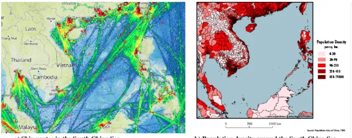
Figure 0 : Socio-economic importance of the South China Sea region 19
Chapter 1 - Introduction 22
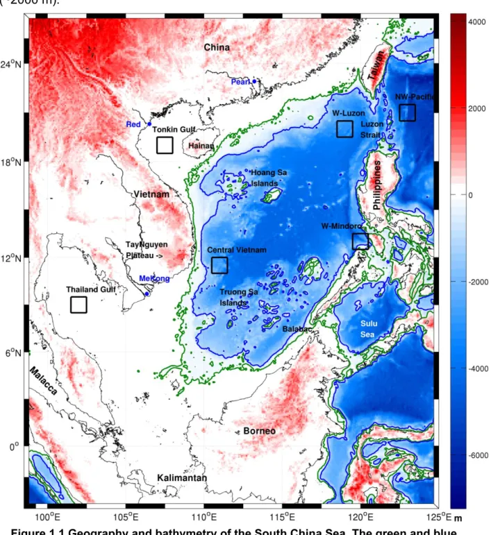
Figure 1.1 Geography and bathymetry of the South China Sea 23
Figure 1.2 Monsoon in the Southeast Asia 24
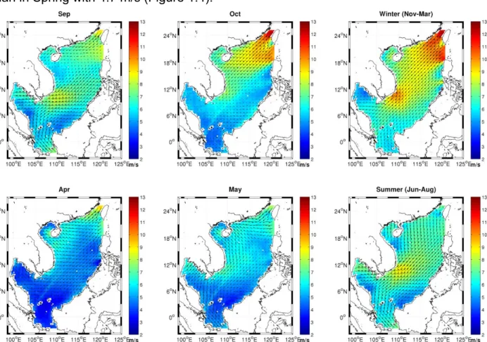
Figure 1.3 Seasonal wind distribution in the SCS 26
Figure 1.4: Annual mean of wind, heat flux and water flux in the SCS 27 Figure 1.5 Climatological seasonal net surface heat and water flux distribution
in the SCS 28
Figure 1.6 Madden Julian Oscillation 29
Figure 1.7 Indian Ocean Dipole 30
Figure 1.8 El Nino Southern Oscillation atmospheric-ocean system 31 Figure 1.9 Kuroshio intrusion observed by altimeter satellite. 32 Figure 1.10 : Climatological monthly freshwater discharges from the Mekong,
Red and Pearl Rivers 33
Figure 1.11 Tidal amplitude of M2, K2, S2 and O1 components in the SCS 34 Figure 1.12 : SCS circulation at different depths in August and December 37
Figure 1.13 Seasonal permanent eddies in the SCS 38
Figure 1.14: Seasonal maps of SST, SSS and MLD in the SCS 41 Figure 1.15: Mean TS profiles from SCSPOD14 dataset at locations
indicated in Figure 1.1 42
Figure 1.16 The SCS domain, locations of TS-profiles and tide gauges,
and August climatological dynamical background 45
Figure 1.17 Impacts of the SVU to regional biomass and climate. 46 Figure 1.18 Schematic summary of the mechanisms of the SVU 47 Figure 1.19 Climatological summer wind and respective Ekman
pumping over the SCS. 49
Figure 1.20 Evidence of the SVU via Meris Chlorophyll and AVHRR SST. 49 Figure 1.21. Wind independent mechanism of the SVU proposed
by Chen et al. 2012. 50
Figure 1.22 Intraseasonal and interannual variability of the SVU via AVHRR SST 51
Chapter 2 - Methods and tool 55
Figure 2.1: Data coverage of the AVHRR SST dataset 55
Figure 2.2 Characteristics of Z and sigma vertical coordinates 60 Figure 2.3 CFSR wind vs. QuikScat and NCAR wind in the SCS 64 Figure 2.4 Inter-comparison of original and corrected CFSR net
heat flux with TropFlux and OAflux 65
Figure 3.2. Eddy kinetic energy between CTRL and ALTI 71
Figure 3.3. Comparison between CTRL and AVHRR SST 72
Figure 3.4. Comparison between CTRL and SCSPOD14 SSS 74
Figure 3.5 A zoom in of Pearl river mouth (Source: Google Map) 75 Figure 3.6: Annual and interannual variation of SST, SSS and
SLA between CTRL and observations 77
Figure 3.7: Comparison between CTRL and SCSPOD14 TS-profiles 80
Figure 3.8. Comparison of CTRL and tide gauges SLA 83
Chapter 4 - Interannual variability of the SVU and contribution of different factors 85 Figure 4.1. Upwelling frequency with respect to different temperature thresholds T0 86 Figure 4.2. Cumulative upwelling intensity in CTRL simulation (maps) 88 Figure 4.3: Upwelling indexes in the CTRL and sensitivity simulations (time series) 90
Figure 4.4: CTRL vs AVHRR SST: individual events 91
Figure 4.5: Geographical locations of upwelling centers in different simulations 93
Figure 4.6. Upwelling and wind relation 102
Figure 4.7. Upwelling and wind relation in different years of CTRL simulation 103 Figure 4.8. Difference of upwelling in CTRL, SimR and SimO
under the same wind conditions 104
Figure 4.9 Offshore upwelling mechanism revealed by CTRL simulation 106 Figure 4.10 Confirmation of offshore upwelling mechanism in different
sensitivity simulations 108
Figure 4.11. Impacts of OIV to the SVU revealed by SimI 109 Figure 4.12 Confirmation of offshore upwelling mechanism in SimI 110 Figure 4.13 Cumulative Vertical positive velocity at 50m over the SVU 112 Figure 4.14 Effectiveness of the SVU in terms of upward vertical water flux. 113
Figure 4.15. Upwelling and ENSO relations 114
Figure 4.16: ENSO vorticity preconditioning mechanisms (time evolution maps) 116 Figure 4.17: Significance of ENSO vorticity preconditioning in
JET+ and OFF+ regions 120
Chapter 5 - Robustness of results in Chapter 4 122
Figure 5.1 : SST biases and trends and the calculation of T0 and
Tref in CTRL, CTRL2 and NoRel 129
Figure 5.2 Cumulative upwelling intensity of CTRL (new method of
computation and new domain) 131
Figure 5.3 Cumulative upwelling intensity of CTRL2 132
Figure 5.4 Cumulative Upwelling intensity of NoRel 132
Figure 5.5: The movement of a strong northern eddy in 1992 133 Figure 5.6 Upwelling vs. wind vs. ENSO: CTRL, CTRL2 and NoRel 135
Chapter 6. Conclusion and future work 137
Figure 6.1 Schematic summary of different mechanisms of the SVU 141
APPENDIX 151
Figure A1.1 - Summer SSS in CTRL, CTRL2 (with Pearl river bay closed) and
SCSPOD14. 151
A2. Influence of Tides 151
Figure A2.1 Comparison of amplitudes of major components
(M2, S2, K1, O1) between Test-0t-a and TPXO7 154
Figure A2.2 Comparisons of phase of K1, O1, M2, S2 between Test-0t-a and TPXO7 155
List of Tables
Table 2.1 Simulation parameters 61
Table 4.1: Quantification of upwelling index: mean and variability 95 Table 5.1 Impacts of relaxation and heat and water flux correction on
Introduction (français)
La Mer de Chine Méridionale (SCS), en Asie du Sud Est, est l’une des plus grandes mers marginales de l’océan mondial, et est le siège d’immenses enjeux économiques, géopolitiques, environnementaux et sociétaux. Selon les estimations de la Banque Mondiale, les régions côtières de la SCS réunissent 26% de la population mondiale et 18% du PIB, et on y observe les densités de population les plus élevées du monde, dépassant les 1000 habitants.km-2. Cette forte densité de population s’accompagne d’un développement économique frénétique, avec une augmentation annuelle du PIB d’environ 6.3% (contre 2.5% à l’échelle mondiale). En 2016, 3370 milliards de dollars de marchandises y ont transité. Cette population, qui dépend en grande partie des ressources maritimes (tourisme, pêche, aquaculture), vit le long des côtes dans des régions de faible élévation, et est donc très fortement soumise aux aléas climatiques : typhons, inondations, sécheresses, oscillation climatique ENSO (El Niño Southern Oscillation), érosion littorale... Une dizaine de typhons traversent la région chaque année (Goh and Chan, 2010). L’événement El Niño exceptionnel de 2015-16 a eu des conséquences dramatiques en Asie du Sud Est : le Sud du Vietnam a ainsi connu la sécheresse la plus intense des 90 dernières années (FAO, 2016), alors que les inondations de 2016 au Nord du Vietnam ont provoqué plus d’une centaine de morts. Le trait de côte dans le delta du Mékong (Sud Vietnam) a reculé de 90 km en 2016, le plus fort recul jamais observé (UNESCAP, 2016). Réciproquement, cette importante activité humaine à de multiples conséquences sur l’environnement littoral, côtier et marin. Ainsi en 2016, le largage accidentel de plus de 300 tonnes de produits toxiques par l’aciérie de Formosa au Nord du Vietnam a conduit à la destruction quasi-totale de la faune et de la flore marine sur plus de 200 km de côtes (Tri et al., 2017). Les conséquences du changement climatique s’y font aussi sentir : le niveau de la mer est monté dans la SCS de 20 cm au cours des 50 dernières années, et la hausse de 1 m prévue pour 2100 provoquerait une disparition de 30 à 50% des terres du Delta du Fleuve Rouge (Duc & Umeyama, 2012). La SCS est donc soumise à des forçages de différentes échelles (de l’événement extrême à la variabilité interannuelle et au changement climatique) et de différentes origines (atmosphérique, océanique, hydrologique et anthropique), et mieux comprendre l’influence de ces forçages est donc un enjeu majeur à l’échelle régionale. C’est également un enjeu à l’échelle globale : la SCS est en effet une région clef dans les échanges de masses d’eau de la circulation thermohaline globale entre l’océan Pacifique et l’Océan Indien (le “South China Sea Throughflow”, SCSTF, Qu et al., 2009).
Ces facteurs de variabilité font intervenir et participent à des interactions complexes entre les différents compartiments du système couplé océan-atmosphère-continent dans cette région. Afin de mieux comprendre ces facteurs et de prévoir et mitiger leurs conséquences, il est essentiel d’améliorer notre connaissance de ce système. Ce travail de thèse s’inscrit dans cette problématique, en s’intéressant à l’une des composantes majeures de ce système, l’océan. L’objectif scientifique général de cette thèse est de mieux comprendre les processus qui gouvernent la dynamique océanique en SCS et leur réponse aux différents facteurs de variabilité. Pour cela, nous nous penchons en particulier sur l’upwelling du Sud Vietnam (SVU).
Le SVU se développe pendant la mousson d’été et joue un rôle majeur dans la dynamique océanique de la région. De plus il y conditionne la productivité biologique et donc les ressources halieutiques, et peut être à l’origine de « marées rouges » (Loick et al., 2007; Dippner et al., 2011). Il présente une forte variabilité quotidienne, saisonnière, et interannuelle. Les études existantes ont suggéré un rôle déterminant du vent dans le déclenchement du SVU et ont émis l’hypothèse de l’influence d’ENSO, et ont également soulevé la question de l’influence des panaches de fleuves et de la marée (Xie et al., 2003 ; Dippner et al., 2007 ; Loick-Wilde et al. 2017…). Par ailleurs, plusieurs études récentes ont mis en évidence dans d’autres régions de l’océan global, et suggéré en SCS, l’impact significatif de la variabilité intrinsèque océanique sur les processus impliqués dans la circulation océanique, liée à son comportement chaotique associé notamment aux structures de (sub)mésoéchelle (voir par exemple Penduff et al., 2011; Li et al., 2014 ; Waldman et al., 2018). Les études précédentes de la circulation en SCS et du SVU ont été effectuées sur de courtes périodes, ou avec des modèles numériques de basse résolution ne permettant pas de résoudre correctement ces structures. Si plusieurs études ont permis d’identifier certains des facteurs qui gouvernent la variabilité du SVU, l’estimation précise de cette variabilité et l’identification des mécanismes physiques associés restent encore à faire, en particulier en ce qui concerne la variabilité interannuelle. Ceci constitue l’objectif précis de cette thèse, qui vise à mettre en place des simulations pluriannuelles à haute résolution, permettant de résoudre la méso-échelle (eddy-resolving) afin d’estimer quantitativement la variabilité interannuelle du SVU ainsi que les contributions respectives des différents facteurs de variabilité (forçage atmosphérique, circulation océanique de grande échelle, panaches des fleuves, marée, variabilité intrinsèque océanique et ENSO), et d’identifier les mécanismes physiques associés.
d’étude (forçages, circulation océanique, variabilité) en abordant d’abord la SCS puis en nous concentrant sur le SVU. Dans le deuxième chapitre nous détaillons les outils et la méthodologie adoptés : observations satellites et in-situ, modèle numérique et stratégie de modélisation. Le troisième chapitre est consacré à l’évaluation du réalisme de notre simulation de référence. Nous analysons les résultats obtenus dans cette simulation de référence ainsi que dans des simulations de sensibilité associées dans le quatrième chapitre, où sont présentés les principaux résultats concernant la variabilité interannuelle du SVU et les mécanismes associés. La robustesse de nos résultats aux choix de configuration du modèle est testée dans le chapitre 5. Nous rappelons les principaux résultats et dressons un inventaire des perspectives de ce travail dans le dernier chapitre de conclusion. L’annexe A2 présente des résultats préliminaires concernant la prise en compte et le rôle de la marée.
Ce document a été rédigé en anglais, mais un résumé, une introduction et une conclusion en français ont été inclus.
Context
The South China Sea (SCS) is a crucial economical-political location of the world. It is a vital route of worldwide goods exchange between large economies including China, Japan, Korea, ASEAN (Association of Southeast Asian Nations), European and American countries (Figure 0a). In 2016, $3.37 trillion worth of goods was transported through the SCS (China Power Team, 2017). It is surrounded by 9 East and South East Asian countries including Vietnam, Cambodia, Thailand, Malaysia, Singapore, Indonesia, Brunei, Philippines and China. According to the World Bank, in 2016, this region accounted for 26.3% of the 7.44 billion world population, and 18% of the $75.845 trillion world GDP (Gross Domestic Production). This is also a fast growing region with a weighted average GDP growth rate of 6.3% compared to 2.5% of the world average in 2016.
Figure 0 : Socio-economic importance of the South China Sea region
SCS coastal areas are among the most densely populated in the world (>1000 hab/km2 in some areas including Vietnam, Figure 0b) because these areas
are particularly adapted to rice production, and due to the presence of marine resources including aquaculture, fisheries, transportation and tourism.These low elevated and densely populated areas are therefore most vulnerable to extreme weather events that hit the region, including typhoons, storm surges, floods and droughts. Human and economic loss due to frequent typhoons (~10/year in the SCS, Goh and Chan, 2010) can result directly from the ocean via storm surges or indirectly via excessive wind strength, rainfall as well as flooding and inland landslide
intra-seasonal (Madden Julian Oscillation, MJO), to inter-annual i.e. Indian Ocean Dipole (IOD) and El Niño Southern Oscillation (ENSO). According to Food and Agriculture Organization (FAO) of the United Nations, in 2016, Vietnam experienced for example its strongest drought in the last 90 years due to El Niño. At larger time scales, climate change has been a hot issue over the last decades. Global warming, earth poles' ice melting, sea level rise and increasing trend of heavy precipitation events in a number of region were reported by the Intergovernmental Panel on Climate Change (IPCC) in 2014. It is essentially important to estimate and forecast regional impacts of climate change, in particular for low elevated and densely populated regions like Vietnam coastal and deltaic regions, which could be hugely impacted by sea level rise.
The fast growing economy in the region also comes with environmental consequences. Under strong economic pressure, environmental damages occurs more often and at larger scales. Industrial pollution is released to the air, soil and water (either to rivers or the ocean) and the air-sea coupled system is an important means of transport of this pollution to larger scales. For example, in April 2016, a Formosa Steel plant located on the coast of Ha Tinh province in Vietnam released more than 300 tons of toxic substance to the ocean which caused massive fish mortality along a 200 km coastal area south of the steel plant (Tri et al., 2017). It impacted millions of people whose income is based on fishing, aquaculture and tourism. This shows that environmental damage can sometimes be more costly than the economic benefits. These damages can be irreversible or take decades to return to their initial state.
Understanding and forecasting the response of the SCS regional coupled atmosphere-ocean-continent coupled system to those sources of variability of different scales and origins is therefore a strong scientific and socio-economic challenge, that requires improvements in our knowledge of the dynamics of this system as well as its tele-connection with other regions in the world. The ocean is one of the key components of the coupled regional system. Better understanding the functioning and variability of the processes that participate to the ocean circulation is therefore essential for a better understanding of the whole system.
This wider scientific objective constitutes the fundamental motivation of this thesis : the objectives of this PhD are to study the governing processes of the SCS dynamics, and their responses to variations in the overlying atmosphere. We focus here on the study of the South Vietnam Upwelling (SVU) – one of the key features of the SCS dynamics in summer, which also impacts on the local marine ecosystems : it is associated with strong primary production which can provide fishing resources to
local people but also induce “red tides” (Loick et al., 2007; Dippner et al., 2011). Thus it represents a direct connection between the natural variability and that influenced by human society, between economic resources and cost. Its variations exhibit multiple time scales (Xie et al., 2003, 2007; Liu et al., 2012; Li et al., 2014), therefore understanding the factors involved in these variations has both a strong scientific and socio-economic stake.
The structure of the thesis is as follow: Chapter 1 gives an overview of the main forcing factors that affect the SCS dynamics including atmospheric forcing, remote oceanic circulation, tidal influence and river input. Then we present the current knowledge of the SCS dynamics, including large scale circulation, mesoscale eddies, thermohaline structure and upwelling systems. In Chapter 2, we describe our methodology as well as the observation data and numerical tools used for this study. Evaluations of the model outputs are shown in Chapter 3. Next, our findings on inter-annual variability of the South Vietnam Upwelling in relation with atmospheric forcing, lateral oceanic forcing, river forcing, ocean intrinsic variability and ENSO are explained in Chapter 4. The robustness of our conclusions to the choices of configuration of the numerical model is examined in Chapter 5. Finally, chapter 6 gives the conclusions and perspectives. Preliminary work concerning the influence of tides on SCS dynamics and SVU is presented in Appendix-A2
Chapter 1: Introduction: forcing factors, circulation
and hydrodynamical processes in the South China
Sea and South Vietnam Upwelling region.
In this chapter we first present a literature review of our current knowledge of the forcing factors and hydrodynamical processes involved in the functioning and variability of the SCS ocean circulation. We then focus on the SVU. We finally present the detailed objectives of this thesis.
1.1 The SCS
1.1.1 Geomorphology - complex topography
The South China Sea (SCS) located south of China and east of Vietnam within about (2.5o S - 25 oN and 99oE - 121 oE) is one of the largest marginal seas in
the world, covering ~ 3.6 million km 2. Figure 1.1 shows the bathymetry of the SCS
plotted using Gebco_08 dataset released by British Oceanographic Data Centre (BODC) in 2010 (www.gebco.net). Almost half of the area of the SCS (1.6 million km2) is shallow shelf with depth < 100m. In the North, the shelf starts from Taiwan
strait then extends southwestward to Hainan with a mean width of about 100km. Then the shelf covers the whole Gulf of Tonkin. In the South, all of the area west of 108oE including the Gulf of Thailand is shallow shelf. The continuity of the northern
and southern shelves is disrupted by the steep continental slope near central Vietnam. The central part of the SCS is deep ocean (depth from 1000 m up to 5000 m), located east of the 110 oE and covering about 1.3 million km2. The SCS has an
average depth of 1000 m.
There are two major groups of islands in the SCS: Hoang Sa (Paracel islands) located at in the northwest of the deep SCS basin and Truong Sa (Spratly Islands) located in the south and southwest of the deep SCS basin. The SCS has many connections with other seas and oceans: with East China Sea and the Pacific in the northeast via Taiwan Strait and Luzon Strait, with Soulu Sea via Mindoro and Balabac strait in the East, with Java Sea in the South via Kalimantan Strait and with Indian Ocean in the Southwest via Malacca Strait. Most of the straits are either shallow and/or narrow with depths < 100m (except Mindoro and Luzon) and widths ranging from 30 km in Malacca Strait to 350 km in Luzon Strait. Of all the straits,
Luzon Strait is by far the most important one with largest width and deepest sill depth (~2000 m).
Figure 1.1 Geography and bathymetry of the South China Sea. The green and blue contours represent isobaths of 100 and 1000 m (data from GEBCO). The black
rectangles represent locations and area (1ox1o) for calculation of mean temperature-salinity profiles in Figure 1.15.
Several mountain ranges with heights up to 2000 m surround the South China Sea and impact on the wind field. The ones along Vietnam, Taiwan and Philippines are perpendicular to the predominant monsoon direction over the SCS (see next section). They can cause a strong orographic effect and thus can induce distinct wind stress curl patterns over the SCS.
Figure 1.2 Monsoon in the Southeast Asia. Climatological seasonal wind at 10m above the sea surface over South East Asia from QuikScat satellite data (2000-2008). Dark
red shaded inland area represent topography > 500m. Red/blue arrows represent summer (JJA) / winter (DJF) wind speed and direction, and contours show the
1.1.2 Forcing systems
a) Atmospheric forcing
The SCS is located inside the Northwestern Tropical Pacific monsoon system (Wang et al., 2009) and is connected to other monsoon systems including the East Asian Monsoon, the Indian Monsoon and the Australian Monsoon. Near the surface, the connections of the SCS monsoon with the other monsoon systems are constrained by land topography. Taiwan Strait, Thailand Peninsula and Kalimantan Strait are the main connections with East Asian, Indian and Australian monsoon systems respectively (Figure 1.2). The summer monsoon (with winds observed by QuikSCAT indicated by red arrows in Figure 1.2) dominates the Indian and Australian monsoons whereas the winter monsoon (winds indicated by blue arrows) dominates the East Asian Monsoon and the Northwestern Tropical Pacific Monsoon. Clearly, the monsoon over the SCS shows a strong and highly seasonal asymmetric reversal.
A more detailed view of this reversal of wind direction from winter to summer in the SCS is shown in Figures 1.3 and 1.4a. The winter monsoon lasts from November to March with almost homogeneous northeast (NE) direction over the whole SCS (Figure 1.3). Its mean speed peaks in December with about 7.8 m/s (Figure 1.4a). The NE wind maximizes at Taiwan, Luzon Strait and Southeast of Vietnam (10-13 m/s). The wind blows eastward over the Thailand Gulf with weakest speed (5-6 m/s), probably due to the shadowing effect of the southern Vietnam land mass in winter. The summer monsoon starts from June with a mean wind speed of 5.5 m/s and peaks in August with a mean wind speed of 6.3 m/s. It veers from southwest (south of 18 oN) to north (north of 18 oN). Wind speed peaks off southern
Vietnam with about 9 m/s and is weakest off the Thailand Peninsula, Borneo and northern central Vietnam where the shadowing effects of land are active. Xie et al. (2003, 2007) proposed that the wind jet off southern Vietnam in summer is due to an orographic effect, passing around TayNguyen Plateau in Southern Vietnam (see Figure 1.1). Fall (Sep-Oct) and Spring (April-May) are two transitional periods for the monsoon. In September, the SW wind is still strong south of 15 oN, while a NE to E
wind starts occurring in the northern part of the SCS. The conflict of wind directions leads to a quiet zone between 16-18 oN. In October, weaker SW to W wind blows
over the southern SCS whereas a strong NE wind prevails in the northern SCS. April is the weakest month in terms of wind speed (4.4 m/s), the NE wind is active over
northern part remains the same. Average wind speed is stronger in Fall with 5.8 m/s than in Spring with 4.7 m/s (Figure 1.4).
Figure 1.3 Seasonal wind distribution in the SCS. Climatological wind speed (color shades, m/s) and direction (arrows) over the SCS for winter and summer and transition periods
Sep-Oct and Apr-May.
The winter monsoon originates from the Siberian High (Wang & He, 2012) and thus is cold and dry; whereas the summer monsoon originates from the Southern Pacific and Indian Ocean (Lau and Yang, 1997; Figure 1.2) and thus is warm and humid. Consequently, the SCS shows a strong seasonal rainfall variability : driest from January to April with net water flux of -1 mm/day i.e. evaporation stronger than precipitation (Figure 1.4b) and wettest in Summer and Fall (~10 mm/day). The transition from Spring to Summer monsoon in the latter half of May is marked by a sudden increase of precipitation over the whole SCS (Lau and Yang, 1997; Wang et al., 2009; Figure 1.4b).
a) b)
Figure 1.4: Annual mean of wind, heat flux and water flux in the SCS. a) Evolution of the 10m above sea level wind speed (blue line) and direction (black arrows with oceanographic convention) averaged over SCS (from QuickScat data 2000-2008). b)
Climatological mean surface net heat flux and water flux over the SCS computed based on NCEP CFSR reanalysis over the period 1991-2004 (Saha et al., 2010).
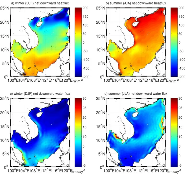
Similar to the wind forcing, the distributions of heat and water fluxes are not homogeneous over the SCS. In winter, the SCS loses heat in the northern part while it continues to gain heat in the south (Figure 1.5a). It gains heat over almost the whole domain in summer with stronger flux in the northern part (Figure 1.5b). There is more rain in the southern SCS from Fall till Spring yet more rain in central SCS in summer (Lau and Yang 1997; Figure 1.5 c,d). This meridional variation of rainfall is related to the movement of Inter-Tropical Convergence Zone (ITCZ) associated with strong convective activities. A seasonal east-west variation of rainfall also occurs due to orographic effects: there is more rain in the western SCS along the Vietnamese coast in winter and more rain in the eastern SCS along the Philippines coasts in summer (Wang et al. 2009; Figure 1.5 c,d). The annual mean values of net heat flux into the SCS varies from one dataset to another. Qu et al. (2009) found a mean value of 23 W.m -2 from COADS dataset (Comprehensive Ocean-Atmosphere
Dataset, Oberhuber 1988) and 49 W.m -2from OAFlux dataset (Yu and Weller, 2007).
The value computed based on NCEP CFSR data for the period 1991-2004 is 64 W.m-2 (Figure 1.4b). Net water flux computed based on this dataset has a mean
value of 1.8 mm/day (Figure 1.4b). Whereas Qu et al. (2009) found that the SCS gains about 0.1 Sv (1 Sv = 10 6 m3.s -1 ) of fresh water from the atmosphere which is
equivalent to about 2.5 mm/day over 3.5 million km 2 area of the SCS. This fresh
water gain leads to a lower sea surface salinity (~1 psu) for the SCS than the surrounding oceans (Qu et al., 2009).
Figure 1.5 Climatological seasonal net surface heat and water flux distribution in the SCS (computed from NCEP CFSR dataset for the period 1991-2004).
The SCS is one of the densest areas for tropical cyclones. From 1965 to 2005, there were 9.8 tropical cyclones each year in the SCS : 60% originated from the neighbouring Pacific and 40% formed locally (Goh and Chan, 2010). Besides the severe impacts in terms of human and economic loss, tropical cyclones are associated with strong impulses of momentum, heat and water exchanges between the ocean and the atmosphere and thus can induce strong intraseasonal variations in the thermohaline structure of the upper layer in the SCS (Chu and Li, 2000; Lin et al. 2003; Tseng et al., 2010; Chang et al., 2010). They can also strongly impact the wind-driven circulation and could possibly impact the South Vietnam Upwelling in summer (Liu et al. 2012). Tropical cyclones occur mostly from June to November when the ITCZ is positioned in the SCS.
Finally, three main climatic phenomena strongly impact the South China Sea climate system : the Madden Julian Oscillation (MJO), the Indian Ocean Dipole (IOD) and the El Niño Southern Oscillation (ENSO). These phenomena influence the fluxes of momentum, heat and water fluxes to the SCS that are associated either with air-sea interactions, river discharge or Luzon Strait Transport at intraseasonal time scale (MJO) and inter-annual time scale (IOD and ENSO).
MJO is named after Madden and Julian who discovered the existence of a stationary oscillation of period from 40-50 days in atmospheric pressure, zonal wind, rainfall etc. in the troposphere (Madden and Julian, 1971, 1972, 1994). This oscillation is due to the eastward movement of a large circulation cell coupled with deep convection in the troposphere of the tropics, and starts in the Indian Ocean moving to the mid Pacific Ocean with a mean speed of 5 m/s (Zhang 2005; Figure 1.6). Zhang and Dong (2004) discovered that the MJO migrates meridionally from south of the equator during boreal winter to north of the equator during boreal summer. Thus over the SCS, the MJO has its most significant impact mainly in summer. Migration of the MJO leads to a northward moving trough (low pressure band) over the SCS. This trough is in phase with the mid-latitude trough in the large scale atmospheric Hadley cell, which can induce westerlies and thus control the onset and strength of summer SW monsoon in the SCS (Tong et al., 2009; Liu et al., 2012). The MJO contributes to about 10% of the intra-seasonal anomalous precipitations over the Southern China Continent in summer (Zhang et al., 2009).
Figure 1.6 Madden Julian Oscillation (after WeatherNation, 2018)
The IOD is associated with a SST dipole that develops between two regions in the Indian Ocean: the western Indian Ocean and off Sumatra (Saji et al., 1999). Positive IOD is characterized by positive anomalous SST over the western Indian
Africa and Indonesia (Saji et al., 1999; Ashok et al., 2001) but also impacts on the onset of the summer monsoon in the SCS and rainfall over China (Yuan et al., 2008; Qiu et al., 2014) : Yuan et al. (2008) suggested that early/late summer monsoon onset over the SCS is due to positive/negative IOD.
Figure 1.7 Indian Ocean Dipole and respective atmospheric circulation and convection activities
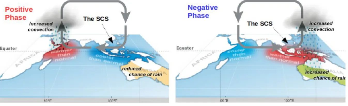
ENSO is a coupled oscillation of SST in the Central Pacific and overlying atmosphere (Trenberth, 1997) at inter-annual time scales. It is the strongest natural mode of the ocean-atmosphere system (Philander, 1985). ENSO has warming/cooling phases called El Niño/La Niña which were originally named due to their positive/negative SST anomalies over the coast of Peru and Ecuador. During the El Niño warming phase, the positive SST anomaly induces cyclonic zonal circulation over the Pacific which weakens trade winds and the monsoon over East Asia (David Neelin and Latif, 1998; Wang et al., 1999; Figure 1.8). During the La Niña cooling phase, negative SST anomalies over the region induce an anti-cyclonic zonal circulation over the Pacific which strengthens trade winds and the monsoon (Philander, 1985; David Neelin and Latif, 1998; Figure 1.8). Over the SCS, many studies have suggested that the SCS summer monsoon is modulated by ENSO such that El Niño/La Niña phases weaken/strengthen the summer monsoon with a later/earlier onset (Lau and Yang, 1997; Chou et al., 2003; Liu et al., 2012; Dippner et al., 2013). Dippner (2013) proposed that the main mechanism whereby ENSO impacts on the summer monsoon in the SCS is via the position of atmospheric trough associated with strong convection in the Inter-Tropical Convergence Zone. Chou et al. (2003) showed that the overall correlation of the SCS summer monsoon and Niño 3.4 index is weak (about 0.5) for the period 1979-2000. This is because in non-ENSO years, other mechanisms modulate the summer monsoon such as the meridional gradient of upper troposphere temperature. In addition, the IOD may also modulate the summer monsoon strength in non-ENSO years (Liu et al.,2012; Dippner 2013). Less is known about the relation between the winter monsoon over the SCS and ENSO. Wang and He (2012) showed that during El Niño/La Niña years,
the East Asian winter monsoon is weakened/strengthened. The connection between the East Asian winter monsoon and the SCS monsoon (Figure 1.2) via Taiwan and Luzon Strait suggest that ENSO may also impacts the SCS winter monsoon.
Figure 1.8 El Nino Southern Oscillation atmospheric-ocean system
b) Oceanic transport through Luzon Strait
The net Luzon Strait Transport (LST) is the inflowing part of the more global South China Sea Through Flow which conveys water from the Pacific through the SCS to East China Sea, Sulu Sea and Java Sea (Qu et al., 2009). Thus it actively contributes to the heat, salt and water balance of the SCS as well as the thermohaline structure inside SCS which will be described in detail in section 1.1.3c. LST varies with time and depth due to different mechanisms. Metzger and Hubert (1996) discovered that the LST consists of barotropic and baroclinic fluxes which are driven by monsoon and gradients of temperature and salinity between Northwestern Pacific water and SCS water respectively. Their sensitivity simulations also showed that wind stress curl and model geometry strongly impact the modeled variability and mean value of LST. In agreement with Metzger and Hubert, a modeling study of Gan et al. (2006) showed that, on the surface, LST is controlled by seasonal monsoons which produce inward/outward flow to/from the SCS. Whereas at greater depth the LST is governed by ageostrophic inward flows due to a westward gradient pressure induced by the Kuroshio Current variations (Gan et al., 2006).
Due to its importance to the SCS dynamics, many studies have attempted to quantify LST using observations (Chu & Li 2000) or modeling (Xue et al., 2004; Qu et al. 2004; Wang et al., 2006c; Fang et al., 2009). These studies showed that the seasonal variability of the LST is controlled by the monsoon with much stronger net LST into the SCS in winter than in summer. However, their findings diverge on the
controlled by the strength of the Kuroshio and during El Niño years, the Kuroshio is weakened and LST is strengthened (Qu et al., 2004; Gan et al., 2006).
Figure 1.9 Mean Absolute Dynamic Topography (units: cm) and the corresponding surface geostrophic currents (units: m/s) derived from the
18-year (1993–2010) satellite altimeter data. Black solid lines represent a schematic of the North Equatorial Current (NEC), Mindanao current and
Kuroshio current - the NMK current system (after Nan et al., 2015).
c) River forcing
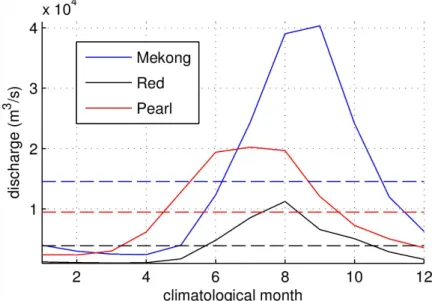
River inputs into the SCS provide a major source of freshwater, sediments and nutrients into the coastal waters and thus are important to the coastal ecosystems and biomass. They also impact on the ocean water masses and dynamics by modifying the salinity. The three major river systems in the SCS are located in the western part where the southeast Asia continent allows the formation of large catchments for the Mekong, Red and Pearl rivers (Figure 1.1). Figure 1.10 shows the climatological discharge computed by compiling available data from Pardé (1938) for the Red River, from the Mekong River Commission (2010) for the Mekong river and from Fekete et al., (2002) for the Pearl river. The Mekong River is the largest one with mean discharge of 14200 m 3s-1. The second is the Pearl River with a
mean annual discharge of 9800 m 3s-1. The Red River is the third with a mean annual
discharge of 3500 m 3s-1. Although the volume of discharge is small compared to the
SCS volume, they can have large scale impacts due to the large scale circulation which can advect fresh water hundreds of kilometers from the river mouth (Gan et
al., 2009). High discharge periods of the three rivers coincide with the SCS summer monsoon (from Spring to Autumn). Variations in discharge are strongly impacted by monsoonal rain (Gao et al., 2015) as well as human impacts (Le et al., 2007; Zhang et al., 2008; Gao et al., 2015) : many dams have been built upstream of these river system for hydropower which leads to a more unnatural regulated flow regime and to a strong decrease of suspended particulate matter at the river mouth (Le et al., 2007).
Figure 1.10 : Climatological monthly freshwater discharges from the Mekong, Red and Pearl Rivers (from respectively Mekong River Commission (2010), Pardé (1938), and
Fekete et al., (2002)).
d) Tidal forcing
Tidal currents and breaking tide-induced internal waves play a crucial role in the ocean mixing at all depths and participate to drive the deep circulation (Stewart 2008). Tidal mixing is particularly strong in shallow areas and can strongly influence coastal sediment transport and mixing in the river mouths. Tidal forcing is thus particularly important in the SCS with 50% of the SCS area covered by shallow shelves and three large river systems including the Mekong, the Red and the Pearl rivers (see figure 1.1) whose maximum discharges exceed 104 m3s-1 (Li et al., 2006;
Wolanski et al., 1998; Mao et al., 2004). Over deep water, however, barotropic tides only have a minor impact on the upper layer thermal structure compared to other forcings (Chang et al., 2010), although there are strong seasonal variations in the internal tide amplitude in the north SCS (Ray and Zaron, 2011).
Figure 1.11 Tidal amplitude of M2, K2, S2 and O1 components in the SCS (Zu et al., 2008)
Due to the small deep basin size of the SCS, barotropic tides in the SCS are mainly transferred from the Pacific via Luzon Strait (Fang et al., 1999; Zu et al., 2008), which is the major connection of the SCS with the large Pacific water body. However, tidal frequency, wavelengths and amplitude are strongly modified by local SCS geometry and bottom topography (Jan et al., 2007; Zu et al., 2008). Zu et al. (2008) found that the amplitude of M2 decreases while the amplitude of K1 increases from the Pacific to the SCS via Luzon Strait. Based on altimetry data, Yanagi et al. (1997) consequently found that tides in the SCS are mostly diurnal, with the ratio (K1 + O1)/(M2+S2) > 1.25 over most SCS area. Shallow shelves and the Tonkin and Thailand gulfs shows stronger variation of tidal amplitude ranging from 0 to 2m compared to homogeneous tidal amplitude in the deep basin (Zu et al., 2008, Figure 1.11). There are several amphidromic points along the Vietnam continental shelf and the two gulfs (Yanagi et al., 1997; Zu et al., 2008; Figure 1.11).
Moreover the interaction of tides with bathymetry can cause partial transformation of the barotropic tide to baroclinic tides e.g. the formation of internal tides in the vicinity of Luzon Strait as observed by Liu et al. (1998), Lien et al. (2005), Zhao et al. (2004) using synthetic aperture radar (SAR) images. Jan et al. (2007) found that about ⅓ of K1 energy is transferred to baroclinic energy while propagating from the Pacific through Luzon Strait. Chang et al. (2010) discovered that internal tides are actually active basin wide. Ray and Zaron (2011) noted that the northern SCS is the only place in the world with a strong seasonal variation in the internal tide amplitudes. Cai et al. (2006), based on sensitivity modeling, suggested the need to include baroclinic tidal effects in modeling studies for a better accuracy of tidal simulations. Including tidal forcing in a ocean general circulation model also improves the ocean thermal structure, circulation and mixing due to the internal tide-current interactions.
1.1.3 The SCS Dynamics
a) Large scale ocean Circulation
The large scale circulation in the SCS is largely driven by the atmospheric monsoon winds system. Previous studies based on modeling (Shaw and Chao 1994) and observations (Wyrtki 1961; Xu et al., 1982; Morimoto et al., 2000; Chu and Li 2000; Fang et al., 2002) found a reversal of the SCS general surface circulation in response to the monsoon reversal. In winter, NE winds induce basin-wide cyclonic surface circulation with an intense southward jet along the western coast. In contrast, weaker summer SW monsoon induces an anti-cyclonic circulation over Southern SCS with a NE western boundary current which turns eastward/offshore between 11-13oN Southern Vietnam, called the eastward jet hereafter. The strength of the jets
can characterize the strength of the seasonal circulations. On average, the winter jet has a mean speed of 0.9 m/s whereas the summer jet has a mean speed of 0.5 m/s. Later studies based on modeling (Wang et al., 2006b; Gan et al., 2006) confirmed the key role of the monsoon but also revealed the important role of Kuroshio intrusions via the Luzon Strait Transport (LST) in the surface circulation, especially in the northern SCS. Intrusion of Pacific water via Luzon Strait maintains the weak cyclonic circulation in summer even though the southwest to south monsoon prevails in the northern SCS (Figure 1.3). Wang et al. (2006b) decomposed the SCS upper layer circulation over the period 1982-2004 using Empirical Orthogonal Function
and characterizes the winter cyclonic SCS circulation. Mode-2 accounts for 27% of the variability and characterizes the summer SCS anti-cyclonic circulation.
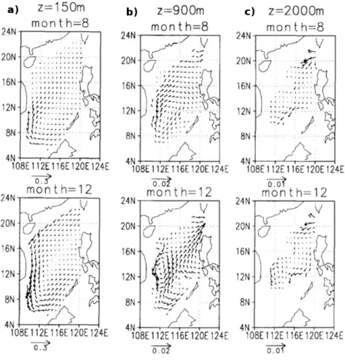
The impact of the surface monsoon forcing is strong down to 150m depth and the seasonal circulation patterns remain similar up to the surface, yet the current speed decreases rapidly with depth (Chao et al 1996; Figure 1.12a). The western boundary current at 150 m depth has a mean speed of about 0.1 - 0.2 m/s. At intermediate depth (900m), modeling outputs from Chao et al. (1996) show a basin-wide anti-cyclonic circulation in August and a northeastward jet of mean speed of 0.005 m/s flowing from the southwest end of the deep basin to Luzon Strait in December (Figure 1.12b). At deep layers (>2000m), the Luzon Strait transport shapes the circulation pattern inside the SCS (Chao et al., 1996; Lan et al., 2015; Figure 1.12c): there is a strong and narrow inward flow in the northern part of the Luzon Strait which leads to a basin-wide cyclonic circulation (Lan et al., 2015).
At interannual time scale, Wang et al. (2006b) suggested that ENSO impacts SCS upper layer circulation via modulation of wind stress curl due to strong correlations between them (they found a strong correlation of 0.92 between time coefficient of mode-1 of wind stress curl and the mode-1 of circulation). They found a 5-month lagged correlation of 0.7 between the time coefficient of the mode-1 and Nino3.4 index over the period 1982-2004, and showed that in El Niño years, upper layer cyclonic circulation is weakened.
There have been very few studies on the impacts of river and tidal forcing on the SCS large scale circulation. Using sensitivity simulations, Chen et al. (2012) suggested that freshwater discharge from the Red river could induce a buoyancy current in the northern SCS along the Vietnamese coast which could meet a tidal rectification current from the south in central Vietnam where the usual NE jet turns offshore, thus participating to the eastward jet formation.
Figure 1.12 : SCS circulation at different depths in August and December (after Chao et al., 1996)
b) Meso-scale structures
Mesoscale eddies with spatial scale of tens to hundreds km and temporal scale of weeks to months are more energetic than the mean circulation (Richardson 1983; Chelton et al., 2007). They are often formed by barotropic/baroclinic instabilities in the mean circulation (Holland, 1978; Qiu and Chen, 2004) over deep water. The SCS has a strong monsoon-driven circulation with impacts of Kuroshio intrusion via the deep Luzon Strait and a deep basin west of Luzon. Mesoscale eddies occur ubiquitously over the SCS and participate to upper layer thermal variability as well as heat and salt flux with the Pacific via Luzon Strait (Wu and Chiang 2007; Chen et al. 2011).
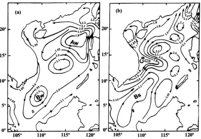
Figure 1.13 Seasonal permanent eddies in the SCS. Permanent eddies Aw, Bw in winter (a) and Bs, Cs in summer (b), after Xu et al., (1982)
In-situ observations in the SCS are generally too sparse to provide comprehensive information about mesoscale activities of the whole SCS basin yet they set our initial understanding of the role of mesoscale eddies in the SCS dynamics. Xu et al. (1982), based on synthesis of available observations, were among the first who discovered the existence of seasonal permanent cyclonic eddies west of Luzon and southeast of Vietnam in winter and of an anticyclonic eddy southeast of Vietnam in paired with a cyclonic eddy off central Vietnam in summer (Figure 1.13). These seasonal permanent eddies are formed in response to the reversal of monsoon in the SCS. Li et al. (1998) showed that eddies originating from the Kuroshio current could transport water of different properties from the Pacific into the SCS. Therefore, eddies play an important role in the exchange of water, heat and salt between the Pacific and the SCS via Luzon Strait. Based on buoy data collected from 1997 to 2000, Chang et al. (2010) concluded that intraseasonal variability of the upper layer thermal structure in central SCS is due to eddy activity.
The great advancements of satellite observations in particular sea surface height (SSH) as well as sea surface temperature (SST) and surface wind have brought new insights of mesoscale activities in the ocean (see Morrow et al., 2017 for a review) including those in the SCS. Using Topex/Poseidon (T/P) sea level anomaly (SLA) data from 1992 - 1997, Morimoto et al. (2000) discovered that both
cold and warm eddies develop in the vicinity of Luzon and propagate westward, meanwhile Wang et al. (2000) found two bands with high mesoscale SLA variability in deep water in the Northern SCS (north of 10 oN): one is along the Vietnamese
coast and the other has a Southwest-Northeast orientation starting from Southeast Hainan to Luzon Strait. Based on blended SLA from multi-mission altimeters and/or modeling, many studies have revealed important characteristics of mesoscale eddies in the SCS: their magnitude, polarity, lifetime, growing phase, breeding ground and traveling path. Wang et al. (2003) proposed that the SCS is anti-cyclonic dominant with eddies generated mainly during and after the cessation of the winter monsoon. Later studies (Xiu et al., 2010; Chen et al., 2011) based on SLA data over a longer period and modeling however showed that there is no significant difference between the number of anticyclonic and cyclonic eddies in the SCS. Xiu et al. (2010) based on modeling and gridded altimeter data from 1993 to 2007 found that 70% of eddies in the SCS have radius smaller than 100 km, and that on average there are about 30 eddies per year. They also found a linear relationship between eddy magnitude, vertical extent and lifetime i.e. stronger eddies have deeper extents and longer lifetimes and vice versa. In addition, Chen et al. (2011), based on 17 years of gridded altimeter data found that eddies generated in different areas have different sizes and lifetimes and that their growing and decaying phase are asymmetric. These studies highlight the ubiquitous presence of mesoscale eddies in the deeper regions of the SCS.
The mechanism for the formation of eddies in the SCS was first investigated by Chu et al. (1998) from sensitivity simulations. They concluded that both wind stress curl and LST can generate deep basin eddies of either polarity. Many other studies highlighted the dominant role of the winter monsoon in eddy genesis either via the wind jet and associated wind stress curl off Luzon or stronger intrusions of Kuroshio waters during winter, making the deep eastern SCS the breeding ground for eddies (Wang et al., 2003; Wu and Chiang 2007; Wang et al., 2008; Chen et al., 2011). The summer orographic induced wind jet and associated wind stress curl was found to be responsible for the generation of eddy dipole off Central Vietnam (Xie et al., 2003; Li et al., 2014). So far, eddy genesis was associated with either wind stress curl or Luzon Strait Transport. To our knowledge, no studies have been conducted to investigate the influence of tidal and river forcing on mesoscale structures generation.
The abundance of mesoscale activities is associated with highly non-linear dynamics and a strong ocean intrinsic variability (OIV, see for example Penduff et
now. Gan and Qu (2008) used an eddy-resolving model and discovered that the summer eastward jet in the SCS has a strong flow variability due to the presence ocean eddies. Li et al. (2014) based on ocean general circulation model (of 1/4 o
resolution) suggested that 20% of the variability of the summer eastward jet could result from nonlinear interactions between the eastward jet and ocean eddies.
c) Thermohaline structure
Under the impacts of the Southeast Asian monsoon and water exchange with the Northwestern Pacific, the thermohaline structure in the SCS shows a strong spatio-temporal variability. Figure 1.14 shows the climatological distribution of SST, sea surface salinity (SSS) and mixed layer depth (MLD) in summer and winter from satellite and in-situ observations. In winter, SST, SSS and MLD show a clear North-South gradient in response to the strong NE monsoon driven surface circulation. This dry and cold NE monsoon promotes evaporation, heat loss and increases the vertical mixing leading to colder SST, higher SSS and deeper MLD in the North than in the South. In addition, the large scale circulation driven by NE-monsoon also brings cold and salty water from the East China Sea and the Pacific via Taiwan and Luzon Straits (see section 1.1.3a). The strong winter jet along Vietnamese coast is visible as a strip of cold SST and high SSS.
In summer, due to higher radiation from the sun, and weaker, warmer and more humid SW summer monsoon coming from the Southern Pacific and the Indian Ocean, the SCS has higher SST associated with strong convection of the overlying atmosphere. The summer monsoon together with atmospheric convection thus bring a lot of precipitation to the SCS (Lau and Yang 1997; Wang et al., 2009). Warmer and fresher upper layers lead to a more stratified upper ocean and thus the MLD is much shallower in summer than in winter (<35m over most of the SCS vs. 35-70 m over deep water in winter). SST, SSS and MLD become spatially more homogeneous with a variation range of 3.5-4 oC, 1.5 - 2 psu and 10-50 m compared
to 10oC, 4 psu and 10 - 70m in winter respectively. SST is higher near continental
shelves and in weak dynamics area. Lowest SST occur in upwelling areas that can be observed on SST maps off the central coast of Vietnam, Northeast of Hainan and in Taiwan Strait. SSS and MLD show higher values in the deep basin than over the shallow shelves.
Figure 1.14: Seasonal maps of SST, SSS and MLD in the SCS. Winter
(December-February) and summer (June-August) averaged SST derived from AVHRR satellite data, SSS and mixed layer depth derived from SCSPOD14 in-situ data set
(Zen et al., 2016)
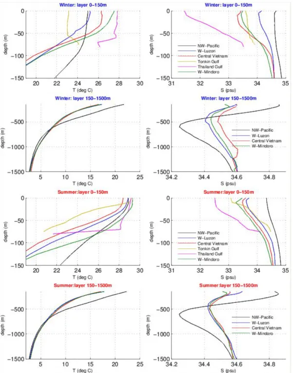
The origin of water masses inside the SCS can be traced back to the northwestern Pacific (Qu et al., 2000; Liu and Gan 2017). Qu et al. (2002) based on Godfrey’s ‘island rule’ and historical observations estimated that, on average, Pacific water intrudes into the SCS via Luzon Strait at a rate of about 4 Sv. To better illustrate the vertical thermohaline structure and its spatio temporal variability inside the SCS, Figure 1.15 shows climatological Temperature - Salinity (TS) profiles at 6 locations: Northwestern Pacific, Western Luzon Strait, Central Vietnam, Tonkin Gulf, Thailand Gulf and Western Mindoro Strait (see Figure 1.1 for locations) computed based on SCSPOD14 dataset (Zeng et al., 2016). To a certain extent, the SCS deep waters replicate TS profiles of the northwestern (NW) Pacific water, yet with strong modifications. In winter, mixed layer depth in the NW Pacific is twice as deep as in the SCS with colder temperature and higher salinity. Western Luzon Strait water shows the closest TS properties to the NW Pacific water. In summer, only the upper layer salinity can distinguish NW Pacific water from the SCS ones. In deeper layers, larger differences of 5 oC and a wider range of salinity exist year-round in NW Pacific
Figure 1.15: Mean TS profiles from SCSPOD14 dataset at locations indicated in Figure 1.1.
Inside the SCS, deep water mean profiles at the western Luzon Strait, Central Vietnam and western Mindoro Strait have a similar shape meaning that the deep SCS basin water is quite well mixed (Figure 1.15). The T/S properties in the shallow gulfs are well mixed over the upper 50 m with extreme T/S values due to their shallowness as well as impacts from nearby rivers (Mekong for Thailand Gulf and Red river for Tonkin Gulf). Tonkin Gulf and Thailand Gulf show the coldest and warmest waters for the upper layer respectively. The salinity in the Thailand Gulf stands out as the freshest water yearound.