HAL Id: inria-00413489
https://hal.inria.fr/inria-00413489
Submitted on 4 Sep 2009
HAL is a multi-disciplinary open access
archive for the deposit and dissemination of
sci-entific research documents, whether they are
pub-lished or not. The documents may come from
teaching and research institutions in France or
abroad, or from public or private research centers.
L’archive ouverte pluridisciplinaire HAL, est
destinée au dépôt et à la diffusion de documents
scientifiques de niveau recherche, publiés ou non,
émanant des établissements d’enseignement et de
recherche français ou étrangers, des laboratoires
publics ou privés.
Schedulability Analysis using Exact Number of
Preemptions and No Idle Time for Real-Time Systems
with Precedence and Strict Periodicity Constraints
Patrick Meumeu Yomsi, Yves Sorel
To cite this version:
Patrick Meumeu Yomsi, Yves Sorel. Schedulability Analysis using Exact Number of Preemptions and
No Idle Time for Real-Time Systems with Precedence and Strict Periodicity Constraints. Proceedings
of 15th International Conference on Real-Time and Network Systems, RTNS’07, 2007, Nancy, France.
�inria-00413489�
Schedulability Analysis using Exact Number of Preemptions and no Idle Time
for Real-Time Systems with Precedence and Strict Periodicity Constraints
Patrick Meumeu Yomsi
INRIA Rocquencourt
Domaine de Voluceau BP 105
78153 Le Chesnay Cedex - France
Email: patrick.meumeu@inria.fr
Yves Sorel
INRIA Rocquencourt
Domaine de Voluceau BP 105
78153 Le Chesnay Cedex - France
Email: yves.sorel@inria.fr
Abstract
Classical approaches based on preemption, such as RM (Rate Monotonic), DM (Deadline Monotonic), EDF (Earliest Deadline First), LLF (Least Laxity First), etc, give schedulability conditions in the case of a single pro-cessor, but assume the cost of the preemption to be negli-gible compared to the duration of each task. Clearly the global cost is difficult to determine accurately because, if the cost of one preemption is known for a given proces-sor, it is not the same for the exact number of preemptions of each task. Because we are interested in hard real-time systems with precedence and strict periodicity constraints where it is mandatory to satisfy these constraints, we give a scheduling algorithm which counts the exact number of preemptions for each task, and thus leads to a new schedu-lability condition. This is currently done in the particular case where the periods of all the tasks constitute an har-monic sequence.
1 Introduction
We address here hard real-time applications found in the domains of automobiles, avionics, mobile robotics, telecommunications, etc, where the real-time constraints must be satisfied in order to avoid the occurrence of dra-matic consequences [1, 2]. Such applications based on automatic control and/or signal processing algorithms are usually specified with block-diagrams. They are com-posed of functions producing and consuming data, and each function has a strict period in order to guarantee the input/output rate as it is usually required by the automatic control theory. Consequently, in this paper we study the problem of scheduling tasks onto a single computing re-source, i.e. a single processor, where each task corre-sponds to a function and must satisfy precedence straints in addition to its strict period. This latter con-straint implies that for such a system, any task starts its execution at the beginning of its period. We assume here that no jitter is allowed at the beginning of each task.
Traditional approaches based on preemption, such as RM (Rate Monotonic) [3], DM (Deadline Monotonic) [4], EDF (Earliest Deadline First) [5], LLF (Least Lax-ity First) [6], etc, give schedulabilLax-ity conditions but al-ways assume the cost of the preemption to be negligible compared to the duration of each task [7, 8]. Indeed, this assumption is due to the Liu & Layland model [9], also called “the classical model”, which is the pioneer model for scheduling hard real-time systems. With this model, the authors showed that a system of independent periodic preemptive tasks with the periods of all tasks forming an harmonic sequence [10]1, is schedulable if and only if:
n
∑
i=1 C0 i Ti ≤1 (1)Ti denotes the period and C0i the inflated worst case
exe-cution time (WCET) with the approximation of the cost of the preemption for taskτi. It is worth noticing that
most of the industrial applications in the field of auto-matic control, image and signal processing consist of tasks with periods forming an harmonic sequence. For exam-ple, the automatic guidance algorithm in a missile falls within this case. Actually, expression (1) takes into ac-count the cost due to preemption inside the value of C0i.
Thus, Ci0=Ci+ε0iwhere Ciis the value of the WCET
with-out preemption, andε0
i is an approximation of the costεi
of the preemption for this task, as explicitly stated in [9]. Thus, expression (1) becomes:
U +ε0 ≤1 (2) where U =
∑
n i=1 Ci Ti, and ε 0 = n∑
i=1 ε0 i TiThe cost of the preemption for taskτi isεi=Np(τi) ·α,
where α denotes the temporal cost of one preemption and Np(τi)is the exact number of preemptions of taskτi.
1A sequence (ai)1≤i≤nis harmonic if and only if there exists qi∈
Nsuch that ai+1=qiai. Notice that we may have qi+16=qi ∀i ∈
Np(τi)may depend on the instance of the task according
to the relationship between the periods of the other tasks in the system. For example, in the case where the periods of the tasks form an harmonic sequence Np(τi)does not
depend on the instance ofτi. Therefore, sinceε0iis an
ap-proximation ofεiand Tiis known,ε0 is an approximation
of the global costε due to preemption, defined by: ε =
∑
ni=1
Np(τi) ·α
Ti
If the temporal cost α of one preemption is known for a given processor, it is not the same for the exact num-ber of preemptions Np(τi) for each taskτi during a
pe-riod Ti. Consequently, it becomes difficult to calculate
the global cost of the preemption, and thus to guaran-tee that expression (2) holds. Obviously the approxima-tion of this latter may lead to a wrong real-time execu-tion whereas the schedulability analysis concluded that the system was schedulable. To cope with this problem the designer usually allows margins which are difficult to assess, and which in any case lead to a waste of resources. Note that the worst-case response time of a task is the greatest time, among all instances of that task, it takes to execute each instance from its release time, and it is larger than the WCET when an instance is preempted. A. Burns, K. Tindell and A. Wellings in [11] presented an analysis that enables the global cost due to preemptions to be fac-tored into the standard equations for calculating the worst-case response time of any task, but they achieved that by considering the maximum number of preemptions instead of the exact number. Juan Echag¨ue, I. Ripoll and A. Cre-spo also tried to solve the problem of the exact number of preemptions in [12] by constructing the schedule using idle times and counting the number of preemptions. But, they did not really determine the execution overhead in-curred by the system due to these preemptions. Indeed, they did not take into account the cost of each preemption during the scheduling. Hence, this amounts to consider-ing only the minimum number of preemptions since some preemptions are not considered: those due to the increase in the execution time of the task because of the cost of the preemptions themselves.
For such a system of tasks with strict periodicity and precedence constraints, we propose a method to calculate on the one hand the exact number of preemptions and thus the accurate value ofε, and on the other hand the sched-ule of the system without any idle time, i.e. the processor will always execute a task as soon as it is possible to do so. Although idle time may help the system to be schedu-lable, when idle time is forbidden it is easier to find the start times of all the instances of a task according to the precedence relation.
The proposed method leads to a much stronger schedu-lability condition than expression (1). Moreover, we do this in the case where tasks are subject to precedence and strict periodicity constraints, using our previous model
[13] that is well suited to the applications we are inter-ested in. Afterwards, to clearly distinguish between the specification level and its associated model, we shall use the term operation instead of the commonly used “task” [14] which is too closely related to the implementation level.
The paper is structured as follows: Section 2 describes the model and gives notations used throughout this paper. Section 3 restricts the study field thanks on the one hand to properties on the strict periods, and on the other hand to properties on WCETs. Section 4 proposes a scheduling algorithm which counts the exact number of preemptions, and derives a schedulability condition, in the case where the periods of all operations constitute an harmonic se-quence. We conclude and propose future work in section 5.
2 Model
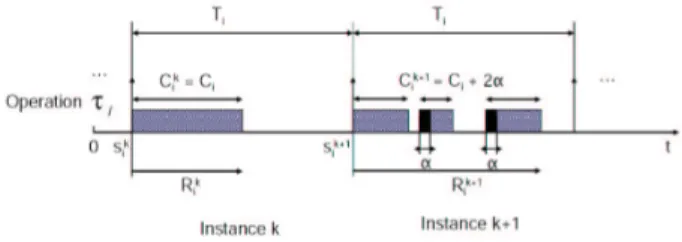
The model depicted in figure 1 is an extension, with preemption, of our previous model [13] for systems with precedence and strict periodicity constraints executed on a single processor.
Figure 1. Model
Here are the notations used in this model assuming all timing characteristics are non-negative integers, i.e. they are multiples of some elementary time interval (for ex-ample the “CPU tick”, the smallest indivisible CPU time unit):
τi= (Ci,Ti): An operation
Ti: Period ofτi
Ci: WCET ofτiwithout preemption, Ci≤Ti
τk
i: The kthinstance ofτi
α: Temporal cost of one preemption for a given processor
Np(τki): Exact number of preemptions ofτiinτki
Ck
i =Ci+Np(τki) ·α: Exact WCET of τiincluding its
pre-emption cost inτk i
s0
i: Start time of the first instance ofτi
sk
i =s0i + (k − 1)Ti: Start time of the kthinstance ofτi
Rk
i: Response time of the kthinstance ofτi
Ri: Worst-case response time ofτi
Ti∧Tj: The greatest common divisor of Tiand Tj,
when Ti∧Tj=1, Tiand Tjare co-prime
τi≺τj:τi−→τj,τiprecedesτj
We denote by V the set of all systems of operations. Each system consists in a given number of operations, with precedence and strict periodicity constraints. Each
operationτiof a system in V consists of a pair (Ci,Ti): Ci
its WCET and Tiits period.
The precedence constraints are given by a partial order on the execution of the operations. τi ≺τj means that
the start time s0
j of the first instance of τj cannot occur
before the first instance ofτi, started at s0i, is completed.
This precedence relation between operations also implies that sk
i ≤skj, ∀k ≥ 1 thanks to the result given in [15]. In
that paper it has been proven that given two operations τi= (Ci,Ti)andτj= (Cj,Tj):
τi≺τj=⇒Ti≤Tj
Regarding the latter relation from the practical point of view, it is worth noticing that when the precedence rela-tions are due to data transfers and the periods of the oper-ations exchanging data constitute an harmonic sequence, the number of operations producing data between two consecutive operations consuming the corresponding data, is constant. Consequently, the number of buffers used to actually achieve the data exchange is bounded, i.e. it can-not increase indefinitely.
The strict periodicity constraint means that two succes-sive instances of an operation areexactly separated by its
period: sk+1
i −ski =Ti ∀k ∈ N, ∀i ∈ {1,··· ,n}, and no
jitter is allowed. In this model the start time is always equal to the release time, in contrast to Liu & Layland’s classical model. A great advantage of the strict periodic-ity constraint for each task is that it is only necessary to focus on the start time of the first instance, the other being directly obtained from it.
It is fundamental to note that, because of the strict peri-odicity constraint and the fact that we are dealing with the single processor case, any two instances of any two op-erations of the system cannot start their executions at the same time.
3 Study field restriction
Firstly, we eliminate all the systems where the start times of any two instances of any two operations are iden-tical. This will be achieved thanks to properties on the strict periods of the operations, using the Bezout theorem. This is formally expressed through both theorems given in section 3.1. Secondly, we eliminate all the systems where the start time of any instance of an operation occurs while the processor is occupied by a previously scheduled op-eration thanks to properties on WCETs of the opop-erations. This is formally expressed through the theorem given in section 3.2. These three theorems give sufficient non-schedulability conditions. For the remaining systems of operations, we adopt a constructive approach which con-sists in building, i.e. in predicting, all the possible preemp-tive schedules without any idle time. In so far, as we are dealing with hard real-time systems whose main feature is predictability, constructive techniques are better suited than simulation techniques based on tests that are seldom exhaustive. In addition, an exhaustive simulation assumes
that there exists a scheduling algorithm, e.g. RM or DM, which is used to perform the simulation. In our case we propose a scheduling algorithm which determines if the system is schedulable and provides the schedule.
3.1 Restriction due to strict periodicity Theorem 1
Given a system of n operations in V , if there are two operations τi = (Ci,Ti) andτj = (Cj,Tj) with (τi ≺τj)
starting their executions respectively at the dates s0
i and s0j
such that
Ti∧Tj=1 (3)
then the system is not schedulable. Moreover, any additional assumption (for example preemption and idle times) on the system intending to satisfy all the constraints is of no interest in this case.
Proof: The proof of this theorem uses the Bezout theorem
and is detailed in [16]. ¥
Theorem 2
Given a system of n operations in V , if there are two operations τi = (Ci,Ti) and τj = (Cj,Tj) with (τi≺τj)
starting their executions respectively at the dates s0
i and
s0
jsuch that
Ti∧Tj| (s0j−s0i) (4)
then the system is not schedulable. Moreover any addi-tional assumption on the system intending to satisfy all the constraints is of no interest in this case.
Proof: The proof of this theorem also uses the Bezout
theorem and is detailed in [16]. ¥
Theorems 1 and 2 give non-schedulability conditions for systems with strict periodicity constraints when both previous relations on the strict periods hold. Moreover, any additional assumption on the system would be useless because of the identical start times of two instances of at least two operations.
We denote byΩλthe sub-set of V excluding the cases
where the strict periods of the operations verify both pre-vious relations.
Ωλ= {{(Ci,Ti)}1≤i≤n∈V / ∀i, j ∈ {1,··· ,n}
∃λ > 1, Ti∧Tj=λ and λ - (s0j−s0i)}
3.2 Restriction due to WCET
The scheduling analysis of a system of preemptive tasks (operations) has shown its importance in a wide range of applications because of its flexibility and its rel-atively easy implementation [17]. Although preemptions may allow schedules to be found that could not be found without it, it can, unfortunately, cause non schedulability of the system due to its global cost.
Since, given two operations τi = (Ci,Ti) and τj =
(Cj,Tj)we haveτi≺τj=⇒Ti≤Tj thus, the operations
corresponding to classical fixed priorities. In other words the smaller the period of an operation is, the greater its pri-ority is, like in the RM scheduling. Note that the schedul-ing analysis of a system of preemptive tasks with fixed priorities has been a pivotal basis in real-time application development since the work of Liu and Layland [9]. Now, we assume that any operation of the system may only be preempted by those previously scheduled, and that any op-eration is scheduled as soon as the processor is free, i.e. no idle time is allowed between the end of the first instance of an operation and the start time of the first instance of the next operation relatively to ≺. This assumption about no idle time allows the greatest possible utilization factor of the processor to be achieved. Therefore, to schedule an operation τi relatively to those previously scheduled,
amounts to filling available spaces in the scheduling with corresponding slices of the exact WCET of τi.
Conse-quently, from the point of view of operationτi the start
time s0
i of its first instance is yielded by the end of the first
instance ofτi−1. Thus, the notion of release time ofτi is
not relevant in this paper, or is equal to s0
i.
A potential schedule
S
of a system is given by a list of the start times of the first instance of all the operations:S
= {(s01,s02, · · · ,s0n)} (5) The start times ski (k ≥ 1, i = 1···n) of the other
in-stances of operationτiare directly deduced from the first
one, and this advantage derives directly from the model. The response time Rk
i of the kth instance of operation
τi= (Ci,Ti)is the time elapsed between its start time ski
and its end time. This latter takes into account the pre-emption thus,
Rki ≥Ci ∀k.
We call Rithe worst response time of operationτi,
de-fined as the maximum of the response times of all its in-stances.
These definitions enable us to say that, in order to sat-isfy the strict periodicity, any operationτi= (Ci,Ti)of a
potentially schedulable system inΩλmust satisfy:
Ri≤Ti ∀i ∈ {1,··· ,n} (6)
We say that a system inΩλhas one overlapping when
the start time of any instance of a given operation occurs while the processor is occupied by a previously scheduled operation. Such systems are not schedulable, as expressed in the following theorem.
Theorem 3
Given a system of n operations inΩλ, if there are two
operations τi= (Ci,Ti) andτj= (Cj,Tj)with (τi≺τj)
starting their executions respectively at the dates s0
i and
s0
jsuch that for k ≥ 1
∃β < k and 0 ≤ (s0j+βTj) − (s0i + (k − 1)Ti) <Rki (7)
then the system is not schedulable. Moreover any addi-tional assumption on the system intending to satisfy all
the constraints is of no interest in this case.
Proof: The proof of this theorem derives directly from
the assumption that an operation may only be preempted by those previously scheduled, and it is detailed in [16]. An example is given below (see figure 2). ¥
Figure 2. System with an overlapping
Now we can partitionΩλinto the three following
dis-joint subsets: the subset Vcof systems with overlappings
which are not schedulable thanks to theorem 3, the subset
Vrof systems with regular operations, i.e. where the
peri-ods of all the operations constitute an harmonic sequence, and the subset Vi of systems with irregular operations.
Thus, since the subset of operations where Ti∧Tj =1
holds, the subset of operations where Ti∧Tj| (s0j−s0i)
holds, and the subset Vc are not schedulable, only the
re-maining subsets Vrand Viare potentially schedulable (see
figure 3). Vc= {{(Ci,Ti)}1≤i≤n∈Ωλ/ ∃i ∈ {1,··· ,n − 1}, ∃j ∈ {i + 1,··· ,n} and 0 ≤ (s0 j+βTj) − (s0i+ (k − 1)Ti) <Rki, k ≥ 1;β ∈ N} Vr= {{(Ci,Ti)}1≤i≤n∈Ωλ/T1|T2| · · · |Tn} Vi=Ωλ\(Vc∪Vr) Figure 3. Ωλ-partitioning
In the remainder of this paper, we restrict our schedul-ing analysis to the subset Vr.
4 Scheduling analysis for V
rGiven any system in Vr, both the exact WCET Cikand
the response time Rk
i of the kth instance of a given
Ci+Np(τi) ·α and Rki =Ri (equal to the worst response
time Riof the operation) because the number of available
spaces left in each instance does not depend on the in-stance itself. Therefore it is worth, in this case, noticing that it is sufficient to give a schedulability condition for the first instance of each operation.
We call Up (respectively Up∗) the pth temporary load
factor (respectively the exact pth temporary load factor)
of the processor (1 ≤ p ≤ n) for a system of n operations {τi= (Ci,Ti)}1≤i≤nin Vr. Up= p
∑
i=1 Ci Ti and U ∗ p= p∑
i=1 C∗ i Ti =Up+ p∑
i=1 Np(τi) ·α TiThis system will be said to be potentially schedulable if and only if:
Un≤1 (8)
and schedulable if and only if:
U∗
n ≤1 (9)
Notice that in (8), Ci is the WCET of operation τi
with-out preemption. From now on, we assume (8) is always satisfied.
We say that the exact WCET C∗
i =Ci+Np(τi) ·α of an
operationτi= (Ci,Ti)of a system in Vris a critical WCET
if its scheduling causes a temporal delay to the start time of the first instance of operationτi+1= (Ci+1,Ti+1),τi≺
τi+1. In other words, this means from the point of view
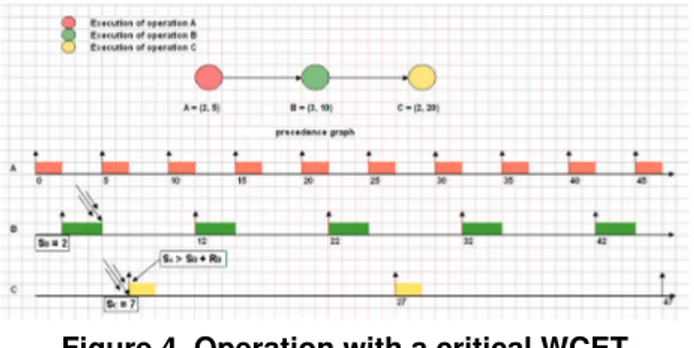
of operationτithat Ci∗is critical when s0i+1>s0i +R1i, see
figure 4. Indeed, in this case the last slice of the exact WCET ofτi exactly fits the next available space in the
scheduling, and thus the first instance of the next operation relatively to ≺ cannot start exactly at the end of the first instance ofτi.
Figure 4. Operation with a critical WCET
In order to make it easier to understand the general case, we first study the simpler case of only two opera-tions. Both cases are based on the same principle which consists, for an operation, in filling available spaces left in each instance with slices of its exact WCET taking into account the cost of the exact number of preemptions nec-essary for its scheduling.
4.1 System with two operations
We considerτ1= (C1,T1)andτ2= (C2,T2)to be a
sys-tem with two operations in Vrsuch as T1|T2.
To be consistent with what we have presented up to now, we will first scheduleτ1, and thenτ2,τ1≺τ2. Hence,
since no idle time is allowed between the end of the first instance ofτ1and the start time of the first instance ofτ2,
we have:
C∗
1=C1 and thus R1=C1 and s02=s01+R1 (10)
Without any loss of generality, we assume in the re-mainder of this paper that s0
1=0. Because the system is
potentially schedulable, we have: µ»R 1+T2 T1 ¼ −1 ¶ ·C1∗+C2≤T2, (11)
i.e. operationτ2 is schedulable without taking into
ac-count the cost of the preemption. Now, on the one hand, if:
C1+C2≤T1
then operationτ2is schedulable without any preemption,
and we have:
C∗
2=C2 and R2=C2 (12)
On the other hand, if:
C1+C2>T1 (13)
then the system requires at least one preemption of oper-ationτ2to be schedulable. To compute the exact number
of preemptions Np(τ2), we perform the algorithm below,
using a sequence of Euclidean divisions.
We denote e = T1−C1and we initialize C1=C2. The
Euclidean division of C1by e gives:
C1=q1·e + r1with q1=
¹C1
e
º
and 0 ≤ r1<e
For all k ≥ 0, we compute
Ck+1=r
k+qk·α (14)
and at each step, we perform the Euclidean division of
Ck+1by e which gives: Ck+1=q k+1·e+rk+1with qk+1= ¹Ck+1 e º and 0 ≤ rk+1<e
We stop the algorithm as soon as: either there exists
m1≥1 such that
m1
∑
i=1
qi·e > T2(1 −U1∗), and thus the
oper-ationτ2is not schedulable in this case, or
∃m2≥1 such that Cm2 ≤e (15)
and thus, Np(τ2)is given by:
Np(τ2) =
m2−1
∑
i=1
Hence
C∗
2=C2+Np(τ2) ·α (17)
and the worst response time R2of the operationτ2is given
by: R2=R02−s02 (18) where: R02=C2∗+ »R0 2 T1 ¼ ·C∗ 1 (19) R0
2is easily obtained by using a fixed point algorithm
ac-cording to: R0,l+12 = C∗ 2+ & R0,l 2 T1 ' ·C∗ 1 ∀l ≥ 0 R0,02 = C2∗ (20) The algorithm is stopped as soon as two successive terms of the iteration are equal:
R0,l+12 =R0,l2 , l ≥ 0 (21) To simplify the notation, the worst response time will be written as: R2= ½ R02=C2∗+ »R0 2 T1 ¼ ·C∗ 1 ¾ −s02 (22)
Therefore a necessary and sufficient schedulability condition for operationτ2, and thus for the system {τ1,τ2}
taking into account the cost of the preemption is given by:
U∗
2 ≤1 i.e., U2+Np(τT2) ·α
2 ≤1 (23)
Example 1
Let τ1 andτ2 be a system with two operations in Vr
with the characteristics defined in table 1:
Table 1. Characteristics of example 4.1
Ci Ti τ1 2 5 τ2 4 10 We have: U2=2 5+ 4 10=0.8 and e = 3.
As operationτ1is never preempted, its worst response
time R1 is equal to its worst-case execution time: R1=
C∗
1=C1=2.
Because τ1≺τ2, these operations are schedulable if
and only if preemption is used (is mandatory).
Although it is not realistic, letα = 1 be the cost of one preemption for the processor in order to show clearly the impact of the preemption. Since C1+C2=6 > T1=5, the
computation of Np(τ2)is summarized in the table below:
Therefore, there is only one preemption Np(τ2) =1
(see figure 5) and C∗
2=4 + 1 · 1 = 5
According to (20), R0
2=9, and the worst response time
R2of operationτ2is given by:
Table 2. computation of Np(τ2)
Steps qi Ci ri
1 1 4 1
2 0 2 2
R2=9 − 2 = 7 and we have R2≤T2=10
Thus the system is schedulable because:
U∗
2=U2+Np(τT2) ·α
2 =0.9 ≤ 1.
Figure 5. Scheduling of two operations 4.2 System with n > 2 operations
The strategy we will adopt in this section of calculating the exact number of preemptions for an operation is dif-ferent from the one used in the previous section, because we can no longer perform a simple Euclidean division. Although, we can perform the Euclidean division to find the number of preemptions for the second operation, this technique cannot be usable for a third operation, and so on. Actually, the available spaces left after having sched-uled the second operation may not be equal, as shown in example 4.2 below, see figure 6.
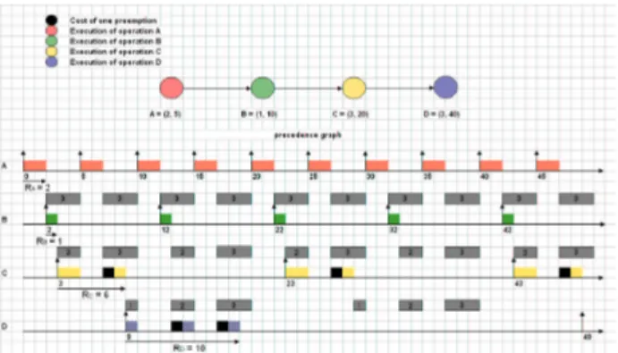
Example 2
Letα = 1 and {τ1,τ2,τ3,τ4} be a system with four
operations in Vrwith the characteristics defined in table 3:
Table 3. Characteristics of example 4.2
Ci Ti
τ1 2 5
τ2 1 10
τ3 3 20
τ4 3 40
The schedule is depicted in figure 6.
In figure 6, it can be seen that after the scheduling of the first operation, the available spaces left have equal lengths (3 time units) but it is no longer the case after the schedul-ing of the second operation, and thus for the third opera-tion after the scheduling of the second operaopera-tion, and so on.
The intuitive idea of our algorithm consists in two main steps for each operation, according to the precedence re-lation. First, determine the total number of available time units in each instance, and then the lengths of each avail-able space (consecutive availavail-able time units). These data
Figure 6. Difficulty of using a simple Eu-clidean division
allow the computation of the instants when the preemp-tions occur. A preemption occurence corresponds to the switch from an available time unit to an already executed one. Second, for each potentially schedulable operation, fill available spaces with slices of its WCET up to the value of its WCET, and then add the cost of the pre-emptions (p ·α for p preemptions) to the current inflated WCET, taking into account the increase in the execution time of the operation because of the cost of the preemp-tions themselves. Finally, the last inflated WCET corre-sponds to the exact WCET. Thus, it is possible to verify the schedulability condition and then whether this opera-tion is schedulable.
Notice that the number of available spaces is the same for all the instances of an operation, thus it is only neces-sary to verify the schedulability condition in the first in-stance which is bounded by the period of the operation. In addition, this verification is performed only once for each operation. Consequently, the complexity of the algorithm even though it has not been yet computed precisely, will actually not explode.
Before going through our proposed algorithm, let us make some assumptions:
1. we will add the cost due to the preemptions to the scheduling analysis of a system if and only if the sys-tem is already schedulable without taking it into ac-count, that is
∑
ni=1
Ci
Ti ≤1.
2. we have scheduled the first j − 1 (2 ≤ j ≤ n − 1) op-erations, and we are about to schedule the jth
opera-tion,
3. we have potentially enough available spaces to schedule operationτj, that is to say:
j−1
∑
i=1 Ã& s0 j+Tj Ti ' − & s0 j Ti '! ·Ci∗+Cj≤TjUnder assumption 2, if Fjdenotes the number of
avail-able time units left in each instance of the operationτj,
then we have:
Fj=Tj· (1 −Uj−1∗ ) (24)
Therefore, the operationτj= (Cj,Tj)is schedulable if
and only if: 0 < C∗
j ≤Fj i.e., C∗j ∈ {1,··· ,Fj} (25)
Let:
L
j= {1,··· ,Fj} (26)L
j denotes the set of all the possible exact WCET C∗j ofoperationτj= (Cj,Tj). Thus, it also contains all the
pos-sible WCETs for operationτj. Once (25) is satisfied, the
worst response time ofτjis given by:
Rj= ( R0 j=C∗j+ j−1
∑
i=1 & R0 j Ti ' ·C∗i ) −s0j (27)and Rjis obtained by using a fixed point algorithm similar
to the one given in the previous section, used to obtain R2.
4.3 Scheduling algorithm
Hereafter is the scheduling algorithm which counts the exact number of preemptions in order to accurately take into account its cost in the schedulability condition. It has the twelve following steps.
1: Determine the start time s0j of the first instance of
operationτj= (Cj,Tj)according to whether the
ex-act WCET C∗
j−1 =Cj−1+Np(τj−1) ·α of operation
τj−1= (Cj−1,Tj−1)is critical or not.
2: Calculate the number of available time units Fj left
in each instance ofτj, and build the set
L
j thanks torelations (24) and (25).
3: Make a first ordered partition of
L
j in kj−1 =TTj j−1sub-sets of equal cardinals such that:
L
j=L
1j∪L
2j∪ · · · ∪L
kj−1 j with ° ° ° ° ° ° ° ° ° ° ° ° ° ° °L
1 j = ½ 1,··· , Fj kj−1 ¾L
2 j = ½ F j kj−1 +1,··· ,2 Fj kj−1 ¾ ...L
kj−1 j = ½ (kj−1−1) Fj kj−1+1,··· ,Fj ¾4: For each subset
L
ij obtained in the previous step,make, if possible, a second ordered partition in hj−1
subsets such that:
L
ij=
L
i,1j ∪L
i,2j ∪ · · · ∪L
i,hj j−1; i = 1,··· ,kj−1where the cardinal of each
L
i,σj with 2 ≤σ ≤ hj−1
equals the cardinal of the subset at the same position in the partition of
L
j−1 starting from the subset withthe greatest pair (kj−2,hj−2)of indices (the subset the
To make this step clear, let us give an example with (kj−2,hj−2) = (2,2).
Let the partition of
L
j−1be such that:L
j−1 =L
1,1j−1∪L
j−11,2 ∪L
2,1j−1∪L
2,2j−1= {1,2} ∪ {3,4,5} ∪ {6,7} ∪ {8,9,10} and let
L
j, and kj−1be such that:½
L
j= {1,2,3,4,5,6,7,8,9,10,11,12}
kj−1=2
Thanks to step 3, we have:
L
j=L
1j∪L
2j whereL
1 j = {1,2,3,4,5,6} andL
2j = {7,8,9,10,11,12} In step 4, we obtain:L
1 j =L
1,1j ∪L
1,2j ∪L
1,3j = {1} ∪ {2,3} ∪ {4,5,6}L
2 j =L
2,1j ∪L
2,2j ∪L
2,3j = {7} ∪ {8,9} ∪ {10,11,12} Thus, at the end of step 4, we can write:L
j= kj−1 [ i=1 hj−1 [ σ=1L
i,σ j (28) 5: Set: ° ° ° ° ° ° ° ° ° ° ° ° ° ° ° ° ° ° ° ° ° ° ° ° ° ° 0 =L
1,1 j 1 =L
1,2j ... hj−1−1 =L
1,hj j−1 hj−1=L
2,1j ... 2hj−1−1 =L
2,hj j−1 2hj−1=L
3,1j ... kj−1hj−1−1 =L
kjj−1,hj−1θ denotes the subset of the possible exact WCETs C∗
j
of operationτj, preemptedθ times. Because
opera-tionτjis potentially schedulable, thus:
∃θ1∈ {0,1,··· ,kj−1hj−1−1} and Cj∈θ1 (29)
Ifθ1=0, then Np(τj) =0. If it is not the case, i.e.
θ16=0, thus we obtain for operationτjthe exact
num-ber of preemptions Np(τj)using the algorithm below:
We initialize C1=Cj q1=θ1 A1=θ
∑
1−1 k=0 card(k) r1=C1−A1 For l ≥ 1, we compute: Bl+1=∑
l k=1 Ak+ (r l+θl·α) (30)If Bl+1 ≤ Fj, thus ∃θl+1 ≥ 0 such that Bl+1 ∈
θ1+ · · · +θl+1. If θl+1 =0, then expression (31)
holds with m2=l + 1 and Np(τj)is given by (32),
else we set: Cl+1=r l+θl·α ql+1=θl+1 Al+1=θ1+···+θ
∑
l+1−1 k=θ1+···+θl card(k) rl+1=Cl+1−Al+1The algorithm is stopped as soon as: either there ex-ists m1≥1 such that Bm1>Fj, and thus operationτj
is not schedulable in this case, or
∃m2≥1 such that θm2=0 (31) and therefore: Np(τj) = m2−1
∑
k=1 qk (32)We compute the exact WCET C∗
j of operationτj:
C∗
j=Cj+Np(τj) ·α (33)
6: Determine the set Ij of all the possible critical exact
WCETs C∗
j of operationτj= (Cj,Tj). Each element
of Ij is the maximum of each subset
L
i,jσ, except Fj,with (1 ≤ i ≤ kj−1)and (1 ≤σ ≤ hj−1)obtained in
step 4.
We distinguish between two types of critical exact WCETs: critical exact WCET of the first order and
critical exact WCET of the second order.
Critical exact WCET of the first order consists of the ordered set I1 j given by: I1j = ©max(
L
ij) for 1 ≤ i ≤ kj−1ª \{Fj} = ½ F j kj−1,2 Fj kj−1, · · · , (kj−1−1) Fj kj−1 ¾Critical exact WCET of the second order consists of the ordered set I2
j given by: I2j = kj−1 [ i=1 I2,ij with I2,ij = nmax(
L
i,σ j ) for 1 ≤σ ≤ hj−1 o \I1jHence Ij=I1j∪I2j and can be rewritten as the ordered
set defined by:
Ij=I2,1j ∪ ½ F j kj−1 ¾ ∪I2,2j ∪ ½ 2 Fj kj−1 ¾ ∪ · · · · · · ∪ ½ (kj−1−1)kFj j−1 ¾ ∪I2,kj j−1 (34)
Again, to make this step clear, let us give an example, using the same one as in step 4. In this step we obtain:
I1
j =©max(
L
1j),max(L
2j)ª \{12} = {6}I2,1j =nmax(
L
1,σj ), 1 ≤σ ≤ 3o\{6} = {1,3}I2,2j =nmax(
L
2,σj ), 1 ≤σ ≤ 3o\{6} = {7,9} Thus, by writing Ijlike in expression (34) we obtain:Ij= {1,3} ∪ {6} ∪ {7,9}
7: Determine whether C∗j is a critical WCET, i.e. C∗j∈Ij,
or not, thanks to step 6.
8: Determine the delay Λj(Cj) that operation τj will
cause to the start time of the first instance of oper-ationτj+1 = (Cj+1,Tj+1). There are three possible
cases for C∗
j:
• C∗j ∈
L
j\Ij, i.e. C∗j is not a critical exact WCET,then:
Λj(Cj) =0 (35)
• C∗j ∈I1j, i.e. C∗j is a critical exact WCET of the first order, then:
Λj(Cj) =s0j (36)
• C∗j ∈I2j, i.e. C∗j is a critical exact WCET of the second order, then:
Λj(Cj) =Λj−1(C0j−1) (37)
such that for each possible value C0,ij ∈I2,ij of C∗j
with (1 ≤ i ≤ kj−1),
Λj(C0,ij )=Λj−1(C0j−1)
where C0
j−1∈Ij−1and C0j−1 is at the same
posi-tion in Ij−1written as in (34) as C0,ij in I2,ij ,
start-ing in Ij−1 from its maximum which belongs to
the sub-set with the greatest pair (2,kj−2)of
in-dices I2,kj−2
j−1 (the subset the furthest on the right).
Again, to make this step clear, let us give an example, using that of step 4. Thanks to everything we have presented up to now, Ij−1=I2,1j−1∪ {5} ∪ I2,2j−1= {2} ∪ {5} ∪ {7} if we assume we had: Λj−1(5) = s0j−1andΛj−1(2) =Λj−1(7) = s0j−2, then as Ij= {1,3} ∪ {6} ∪ {7,9}
In this step we obtain: Λj(6) = s0j because 6 ∈ I1j Λj(3) =Λj(9) =Λj−1(7) = s0j−2 Λj(1) =Λj(7) =Λj−1(5) = s0j−1
9: Calculate the worst response time Rj of operationτj
thanks to expression (27).
10: Increment j: j ← j + 1 and determine the start
time s0
j+1 of the first instance of operation τj+1 =
(Cj+1,Tj+1) according to whether operation τj =
(Cj,Tj)has a critical exact WCET C∗j, or not.
s0j+1=Rj+s0j+Λj(Cj) (38)
11: Go back to step 2 as long as there remain potentially schedulable operations.
12: Give the necessary and sufficient schedulability con-dition: U∗ n ≤1 i.e., Un+ n
∑
i=2 Np(τi) ·α Ti ≤1 (39)and the valid schedule
S
for the system taking into account the global cost due to preemptions:S
= {(s01,s02, · · · ,s0n)} (40)Example 3
Letα = 1 and {τ1,τ2,τ3,τ4}be a system with four
op-erations in Vr with the characteristics defined in table 4.
Table 4. Characteristics of example 4.3
Ci Ti
τ1 2 5
τ2 1 10
τ3 3 20
τ4 3 40
That system is potentially schedulable, indeed:
U4=2 5+ 1 10+ 3 20+ 3 40=0.725
The scheduling algorithm that we introduced previously gives: C∗
1=2,C∗2=1,C3∗=4,C4∗=5, thus:
U∗
4 =25+101 +204 +405 =0.825
and we obtain (see figure 7):
Figure 7. Scheduling algorithm
In figure 7, for each operation, we can see its actual exact WCET (squared), its critical exact WCET (circled), and its exact number of preemptions.
The global cost due to preemption is given by: pr = 1 10·0 + 1 20·1 + 1 40·2 = 0.1 and therefore the schedulability condition is:
U∗
4 =U4+pr = 0.825 ≤ 1
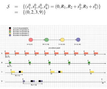
The valid schedule of the system of operations obtained with our scheduling algorithm is given in figure 8, and is such that:
S
= {(s01,s20,s03,s04) = (0,R1,R2+s02,R3+s03)}= {(0,2,3,9)}
Figure 8. Preemptions taken into account
5 Conclusion and future work
We are interested in hard real-time systems with prece-dence and strict periodicity constraints where it is manda-tory to satisfy these constraints. We are also interested in preemption which offers great advantages when seek-ing schedules. Since classical approaches are based on an approximation of the cost of the preemption in WCETs, possibly leading to a wrong real-time execution, we pro-posed a constructive approach so that its cost may be taken into account accurately. We proposed a scheduling algo-rithm which counts the exact number of preemptions for a system in Vrwhich is the subset of systems where the
pe-riods of all operations constitute an harmonic sequence as presented in section 3.2, and thus gives a stronger schedu-lability condition than Liu & Layland’s condition.
Currently, we are seeking a schedulability condition for systems in Viwhich is the subset of systems with irregular
operations and we are planning to study the complexity of our approach in both Vr and Vi. Moreover, because idle
time may increase the possible schedules we also plan to allow idle time, even though this would increase the com-plexity of the scheduling algorithm.
References
[1] Joseph Y.-T. Leung and M. L. Merrill. A note on preemp-tive scheduling of periodic, real-time tasks. Information
Processing Letters, 1980.
[2] Ray Obenza and Geoff. Mendal. Guaranteeing real time performance using rma. The Embedded Systems
Confer-ence, San Jose, CA, 1998.
[3] J.P. Lehoczky, L. Sha, and Y Ding. The rate monotonic sheduling algorithm: exact characterization and average case bahavior. Proceedings of the IEEE Real-Time Systems
Symposium, 1989.
[4] N.C. Audsley, Burns A., M.F. Richardson, and A.J. Wellings. Hard real-time scheduling : The deadline-monotonic approach. Proceedings 8th IEEE Workshop on
Real-Time Operating Systems and Software, 1991.
[5] H. Chetto and M. Chetto. Some results on the earliest dead-line scheduling algorithm. IEEE Transactions on Software
Engineering, 1989.
[6] Patchrawat Uthaisombut. The optimal online algorithms for minimizing maximum lateness. Proceedings of the
9th Scandinavian Workshop on Algorithm Theory (SWAT),
2003.
[7] M. Joseph and P. Pandya. Finding response times in real-time system. BCS Computer Journal, 1986.
[8] Burns A. Tindell K. and Wellings A. An extendible ap-proach for analysing fixed priority hard real-time tasks. J.
Real-Time Systems, 1994.
[9] C.L. Liu and J.W. Layland. Scheduling algorithms for mul-tiprogramming in a hard-real-time environment. Journal of
the ACM, 1973.
[10] Tei-Wei Kuo and Aloysius K. Mok. Load adjustment in adaptive real-time systems. Proceedings of the 12th IEEE
Real-Time Systems Symposium, 1991.
[11] Tindell K. Burns A. and Wellings A. Effective analysis for engineering real-time fixed priority schedulers. IEEE
Trans. Software Eng., 1995.
[12] I. Ripol J. Echage and A. Crespo. Hard real-time preemp-tively scheduling with high context switch cost. In
Pro-ceedings of the 7th Euromicro Workshop on Real-Time Sys-tems, 1995.
[13] L. Cucu, R. Kocik, and Y. Sorel. Real-time scheduling for systems with precedence, periodicity and latency con-straints. In Proceedings of 10th Real-Time Systems
Con-ference, RTS’02, Paris, France, March 2002.
[14] J.H.M. Korst, E.H.L. Aarts, and J.K. Lenstra. Scheduling periodic tasks. INFORMS Journal on Computing 8, 1996. [15] L. Cucu and Y. Sorel. Schedulability condition for systems
with precedence and periodicity constraints without pre-emption. In Proceedings of 11th Real-Time Systems
Con-ference, RTS’03, Paris, March 2003.
[16] P. Meumeu and Y. Sorel. Non-schedulability conditions for off-line scheduling of real-time systems subject to prece-dence and strict periodicity constraints. In Proceedings
of 11th IEEE International Conference on Emerging tech-nologies and Factory Automation, ETFA’06, WIP, Prague,
Czech Republic, September 2006.
[17] Radu Dobrin and Gerhard Fohler. Reducing the number of preemptions in fixed priority scheduling. In 16th
Euromi-cro Conference on Real-time Systems (ECRTS 04),