Pricing bivariate option under GARCH-GH model with dynamic copula: application for Chinese market

HAL Id: halshs-00368336

https://halshs.archives-ouvertes.fr/halshs-00368336

Submitted on 15 Apr 2009

HAL is a multi-disciplinary open access archive for the deposit and dissemination of sci-entific research documents, whether they are pub-lished or not. The documents may come from teaching and research institutions in France or abroad, or from public or private research centers.

L’archive ouverte pluridisciplinaire HAL, est destinée au dépôt et à la diffusion de documents scientifiques de niveau recherche, publiés ou non, émanant des établissements d’enseignement et de recherche français ou étrangers, des laboratoires publics ou privés.

dynamic copula: application for Chinese market

Dominique Guegan, Jing Zhang

To cite this version:

Dominique Guegan, Jing Zhang. Pricing bivariate option under GARCH-GH model with dynamic copula: application for Chinese market. European Journal of Finance, Taylor & Francis (Routledge), 2009, 15 (7-8), pp.777-795. �10.1080/13518470902895344�. �halshs-00368336�

Model with Dynamic Copula: Application for

Chinese Market

D. Gu´egan1 and J. Zhang2 1

PSE, CES-MSE, University Paris1 Panthon - Sorbonne, 106 bd de l’hopital, 75013 Paris, France.

dguegan@univ-paris1.fr

2 _{East China Normal University, Department of Statistics}

3663, Zhongshan North Road, 200063 Shanghai, China. celine chang 12@hotmail.com

Abstract. This paper develops the method for pricing bivariate contin-gent claims under General Autoregressive Conditionally Heteroskedastic (GARCH) process. In order to provide a general framework being able to accommodate skewness, leptokurtosis, fat tails as well as the time varying volatility that are often found in financial data, generalized hyperbolic (GH) distribution is used for innovations. As the association between the underlying assets may vary over time, the dynamic copula approach is considered. Therefore, the proposed method proves to play an important role in pricing bivariate option. The approach is illustrated for Chinese market with one type of better-of-two markets claims: call option on the better performer of Shanghai Stock Composite Index and Shenzhen Stock Composite Index. Results show that the option prices obtained by the GARCH-GH model with time-varying copula differ substantially from the prices implied by the GARCH-Gaussian dynamic copula model. Moreover, the empirical work displays the advantage of the suggested method.

Keywords:call-on-max option; GARCH process; generalized hyperbolic (GH) distribution; normal inverse Gaussian (NIG) distribution; copula; dynamic copula

1 Introduction

Following the great work of BS73 and MR73, the option pricing literature has been developed a lot. Over the years, various generalizations of the Brownian motion framework due to BS73 have been used to model multi-variate option prices. Examples include MW78, SRM82, JH87, RE92, and SDC94. In all these papers, correlation was used to measure the depen-dence between assets. However, EMS02 and FR02 have pointed out that, correlation may cause some confusion and misunderstanding. Indeed, it is a financial stylized fact that correlations observed under ordinary market differ substantially from correlations observed in hectic periods.

On the other hand, to take into account the heteroskedasticity of assets returns, a lot of models have been put forward, such as the constant-elasticity-of-variance model of CJ75, the jump-diffusion model in MR76, the compound-option model in GR79 and the displaced-diffusion model in RM83. Opposed to the aforementioned models, a bivariate diffusion model for pricing option on assets with stochastic volatilities was introduced by HW87. Unfortunately, the bivariate diffusion option model requires the conditions stronger than no arbitrage and it faces the difficulty in empir-ical study that the variance rate is unobservable.

Through an equilibrium argument, DJC95 showed that options can be priced when the dynamics for the price of the underlying asset follows a GARCH process. This GARCH option pricing model has so far experi-mented some empirical successes in HKV94, DJC96 and HN00. In order to extend the risk neutralization developed in RM76 and BM79, DJC99 developed the GARCH option pricing model by providing a relatively easy transformation to risk-neutral distributions.

Now the distribution of the error term in GARCH process attracts a lot of attention. In ERF82 the normal distribution is used but alterna-tive distributions such as the t distribution or the GED distribution have been considered to capture the excess kurtosis and fat tails. Unfortu-nately, as explained in DJC99, using t distribution to model continuously compounded asset returns is inappropriate, since the moment generating function of t distribution with any finite degree of freedom does not exist, and because of the symmetry of the GED distribution, a more flexible appropriate distribution is called for.

In JL01, SL06 and CHJ06, it was found that the normal inverse Gaussian (NIG) models, the special case of generalized hyperbolic (GH) distribu-tion, are able to outperform some of the most praised GARCH models when considering daily U.S. stock return data. In particular, a big gain is found in modelling the skewness of equity returns as in EK95 and EP02. It is concluded that allowing conditional skewness leads to more accurate predictions of conditional variance and excess return. Moreover, GH dis-tribution has the moment generating function, which gains an advantage over the t distribution.

As multivariate options are regarded as excellent tool for hedging the risk in today’s finance, a more appropriate measure for dependence structure is required, here we concentrate on the copula. Copulas are functions that join or “couple” multivariate distribution functions to their one-dimensional marginal distribution functions, JH97 and NR99. It has been known since the work of SA59 that any multivariate continuous distribu-tion funcdistribu-tion can be uniquely factored into its marginals and a copula. In a word, copula has proven to be an interesting tool to take into account all the dependence structure and even to capture the nonlinear dependence of data set.

Copulas have also been introduced to price bivariate options as shown in RJV99, CL02. In these papers, all the appropriate preliminary copulas are supposed to remain static during the considered time period. How-ever, most of data sets often cover a reasonably long time period and economic factors induce changes in dependence structure. Thus the basic properties of financial products change in different periods (the stable period and the crisis period). Therefore, to price the bivariate option in a robust way, a dynamic copula approach should be adopted.

In the present paper, a new dynamic approach to price the bivariate op-tion under GARCH-GH process using time-varying copula is proposed. Through fitting two GARCH-GH models on two underlying assets, the return innovations are obtained. Observing that the dependence structure for the two series of innovations changes over time, we analyze the changes in copulas through moving windows. Then a series of copulas are selected on different subsamples according to AIC criterion [][]AH74. Through this method, the changes of the copula can be observed and the change trend appears more and more clearly. Conditioning on the result of the moving window process, the dynamic copula with time-varying parameter is

ex-pressed similarly as in DE03, JR04, GTP06, PAJ06, GGW05 and GZ06 for instance. An innovating feature of the present paper is investigat-ing the dynamic evolution of the copula’s parameter as a time-varyinvestigat-ing function of predetermined variables, which gives a considerably dynamic expression to the changes of the copula and makes the changes of param-eters more tractable.

In the empirical study, call option on the better performer based on two important Chinese equity index returns (Shanghai Stock Composite Index and Shenzhen Stock Composite Index) is used to illustrate the innova-tive method described previously. The Student t copula is the best fitting copula and time-varying parameter is considered. We provide the option prices implied by GARCH-NIG model with time-varying copula and these prices are compared with those obtained by GARCH-Gaussian model. It can be observed that the prices implied by the GARCH-Gaussian are generally underestimated.

The remainder of this paper is organized as follows. In Section 2, the basic framework of option pricing is recalled and the notations are intro-duced. Section 3 introduces the time-varying copula for pricing bivariate options using marginals GH distributions. In section 4, empirical study is described and results are provided. Section 5 concludes. In an Annex we provide the expression of Gaussian and Student t copulas.

2 Preliminaries and Related Works

We specify the framework for option pricing that we choose, then we introduce the model with which we work and the innovation distribution that we use.

2.1 Option valuation

This paper concentrates on European option on the better performer of two assets, but the technique is sufficiently general to be applied for other alternative multivariate options as well. The call option on the better performer belongs to one type of better-of-two markets and can be referred to as call-on-max option. The payoff of a unit amount call-on-max option is

max{max(S1(T ), S2(T ))− K, 0},

where Si is the price at maturity T of the i-th asset (i = 1, 2), and K

i-th index (i = 1, 2) from time t_{− 1 to time t, and the corresponding} log-return is denoted as ri,t = log(Ri,t).

The fair value of the option is determined by taking the discounted ex-pected value of the option’s payoff under the risk-neutral distribution. As the call-on-max is typically traded over the counter, price data are not available. Therefore, valuation models cannot be tested empirically. How-ever, comparing models with different assumptions can be implemented.

The approach of BS73 for option pricing assumes the efficiency of the financial market and all the pricing theory developed after their seminal work lies on the existence of the risk neutral measure. This measure ver-ifies the martingale property for the theory of contingent claim pricing. Recently, some works have proposed new approaches for pricing, based on historical measure. These new works are really interesting because they are close to the reality, see for instance BAEM04. Nevertheless, the present work keeps a historical approach for pricing options using the risk-neutral environment.

2.2 Generalized Hyperbolic (GH) distributions

In order to take into account specific stylized fact of the assets (skewness and kurtosis mainly), we will work with the generalized hyperbolic (GH) distribution that we present briefly now. We refer to EK95 for more de-tails.

The one dimensional generalized hyperbolic distribution admits the fol-lowing density function

fGH(x; λ, α, β, δ, µ) = κ(λ, α, β, δ)τ(λ−1/2)Kλ−1/2(ατ ) exp(β(x−µ)), (1)

where Kλ is the modified Bessel function of the third kind and

κ(λ, α, β, δ) = (α 2_{− β}2₎λ/2 √ 2παλ−1/2_δλ_K λ(δpα2− β2) , τ =pδ2_{+ (x− µ)}2_, and x∈ R.

The parameters λ, α, β, δ, µ _{∈ R are interpreted as follows: µ ∈ R is the} location parameter and δ > 0 is the scale parameter. The parameter

0_{≤ |β| < α describes the skewness and α > 0 gives the kurtosis.} Particu-larly, if β = 0, the distribution is symmetric, and if α→ ∞, the Gaussian distribution is obtained in the limit. The parameter λ _{∈ R characterizes} certain subclasses of the distribution and considerably influences the size of the probability mass contained in the tails of the distribution. If the random variable x is characterized by a generalized hyperbolic distribu-tion, we denote it x ∼ GH(λ, α, β, δ, µ).

Generally we will use in applications the parameters ¯α = αδ and ¯β = βδ corresponding to the scale and location invariant parameters. Then, the density function of the generalized hyperbolic distribution expressed in terms of the invariant parameters becomes:

fGH(x; λ, ¯α, ¯β, δ, µ) = κ(λ, ¯α, ¯β, δ)χ(λ−1/2)Kλ−1/2(¯αχ) exp( ¯β( x− µ δ )), (2) where κ(λ, ¯α, ¯β, δ) = (¯α 2_{− ¯β}2₎λ/2 √ 2π ¯αλ−1/2_δλ_K λ(p ¯α2− ¯β2) , χ = r 1 + (x− µ δ )2,

and x _{∈ R. In that case, GH(λ, ¯}α, ¯β, δ, µ) is a location-scale distribution family, and we have

x ∼ GH(λ, ¯α, ¯β, δ, µ)_⇔ x− µ

δ ∼ GH(λ, ¯α, ¯β, 1, 0). (3) A special case of the GH distribution is the Normal Inverse Gaussian (NIG) distribution obtained by assuming that λ =−1/2 in Equation (1). The density function of the NIG distribution expressed in terms of the invariant parameters ¯α = δα and ¯β = δβ is equal to:

fN IG(x; ¯α, ¯β, δ, µ) = ¯ α πδexp[ q ¯ α2_{− ¯β}2_{+ ¯β(}x− µ δ )] K1(¯α q 1 + (x−µ_δ )2₎ q 1 + (x−µ_δ )2 , (4) where x, µ _{∈ R, δ > 0 and 0 < | ¯}β_{| < ¯}α. If the random variable x has a NIG distribution, we denote it as x ∼ NIG(¯α, ¯β, δ, µ). In the next ap-plication, we will use this particular case of the generalized hyperbolic distribution.

2.3 GARCH process transformation

Here we are interested in pricing options, thus we need to derive the joint risk-neutral return process from the objective bivariate distribution. Instead of deriving the bivariate risk-neutral distribution directly, we pro-pose to transform each of the marginal process separately.

First of all, we assume that the one-period log-return for every index, under probability measure P , follows a GARCH process, that is, for i = 1, 2:

ri,t = r + λphi,t− 1/2hi,t+ εi,t,

where εi,t has mean zero and conditional variance htunder the historical

measure P ; r is the constant one-period risk-free rate of return and λ the constant unit risk premium (note that under conditional lognormality, one plus the conditionally expected rate of return equals exp(r + λphi,t).

It just suggests that λ can be interpreted as the unit risk premium). We further assume that εi,t follows a GARCH(p,q) process of Bollerslev

(1986) under measure P . Thus formally, we have:

εi,t|ϕi,t−1∼ D(0, hi,t) under measure P,

where D(.) can be the Gaussian law or any more general distribution func-tion FD, with zero mean and variance hi,t and, ϕi,t−1 is the information

set of all information up to and including time t− 1. Then,

hi,t= αi,0+ q X j=1 αi,jε2i,t−j + p X j=1 βi,jhi,t−j.

Some parameter restrictions are p _{≥ 0, q ≥ 0; α}i,0 > 0; αi,j ≥ 0(j =

1, . . . , q); βj ≥ 0(j = 1, . . . , p) and Pqj=1αi,j +Ppj=1βj < 1 to ensure

covariance stationarity of the GARCH (p, q) process.

In order to develop the GARCH option pricing model and finally obtain the risk-neutral price, we follow the methodology of DJC99, assuming that (εt)t follows a NIG distribution that takes into account the skeness and

the leptokurticity observed inside the distribution function of the real data sets. We recall the definition of the LRNVR principe introduced in Duan (1995) and provide the model under Q. We say that a pricing measure Q satisfies the locally risk-neutral valuation relationship (LRNVR) if the measure Q is absolutely continuous with respect to the measure P , and then ritconditionally to ϕi,t−1is distributed lognormally (under Q) with:

and

varQ[ri,t|ϕi,t−1] = varP[ri,t|ϕi,t−1],

almost surely with respect to measure P .

In the previous definition, the conditional variance under the two mea-sures are required to be equal. This is necessary to estimate the condi-tional variance under P . This property and the fact that the condicondi-tional mean can be replaced by the risk-free rate yield a well specified model that does not locally depend on preferences. This latter fact is proved in Duan (1995). Here we will reduce all preference consideration to the unit risk premium. Since Q is absolutely continuous with respect to P , the al-most sure relationship under P also holds true under Q. Note that in this study we restrict to constant interest rate assumption even if stochastic interest rates can be considered, but then the resulting model are more complicated. It is not the purpose of this paper which focus mainly on the bivariate pricing and the use of dynamical copula.

The strategy develop by Duan (1999) to get a generalized version of the GARCH option pricing model is based on a transformation that is capable of converting the fat tailed and /or skewed random variables into normally distributed ones. We follow the same idea inside this paper for the trans-formation of each asset which is an approximately extension of the result obtained in Gaussian case, for a GARCH - GH model. Thus, assuming that the GLRNVR principle is verified, the assets returns processes which follow a GARCH model under measure P can be characterized approxi-mately by a simple risk-neutral dynamic GARCH model under measure Q defined such that:

ri,t = r + λphi,t− 1/2hi,t+ ηi,t, (5)

where

ηi,t= F_D−1[Φ(Zi,t− λ)],

where Zi,t, conditional on ϕi,t−1, is a Q-standard normal random variable

and Φ(·) denotes the standard normal distribution function, and

hi,t = αi,0+ q

X

j=1

αi,j(ηi,t− λphi,t−j)2+

p

X

j=1

βi,jhi,t−j, (6)

The previous relationships imply that the log-return ri,t follows a process

close to a GARCH (p, q) under the risk-neutral measure. We use this ap-proximation which provides a relatively easy transformation to generalize

local risk-neutral distributions that is skewed and leptokurtic. According to this expression, the terminal asset price can be derived

Si,T = Si,texp[(T − t)r − 1/2 T X s=t+1 hi,ts+ T X s=t+1 ηi,s] (7)

Considering the importance of the martingale property for the theory of contingent claim pricing, it is necessary to note that the discount asset price process e−rtT_S

i,T is a Q-martingale. Therefore, under the GARCH

specification, the call-on-max option, with exercise price K at maturity T , has the time-t value given by

COMt= e−

PT

s=t+1rsEQ[max{max(S

1,T, S2,T)− K, 0}]. (8)

This equation provides the fair value for call-on-max option.

Now we are interested to get the multivariate distribution for this bi-variate option. Since the dynamic of ri,t with respect of the measure Q

is completely characterized by (5), the valuation problem reduces to the task of computing the expectation in (7). To get it, we can use Monte Carlo simulation to generate many sample paths in accordance with the previous system and take the discounted average of the contract payoff to yield the price for the derivative claim in question. The algorithm is provided in Subsection 4.3.

In this part, we consider a classical GARCH modelling for the underlying assets, but clearly it is possible to extend this approach to asymmetric GARCH processes, like the EGARCH model NDB91, the GJR model GJR93 and the A-PARCH model DGE93, for instance.

The previous exercise mainly developed in Duan (1995) under Gaussian distribution has been extended for other GARCH model, with specific kernel pricings, with other distribution functions like the mixing Gaus-sian distribution, Gourieroux and Monfort (2007), the NIG distribution, Gerber and Siu (1994), the Generalized hyperbolic distributions, Christof-fersen et al. (2006). The work of Duan (1999) - on which this exercise is based - appears as a particular case of these previous cited works which assume an exponential affine parametrization for the stochastic discount factor. Now, the general result obtained recently by Chorro, Gu´egan and Ielpo (2008a) applied on GARCH-GH model confirms the interest of the empirical approach developed here. Indeed, the authors - following a lot

of works in the literature - show that if the returns are governed by any GARCH-GH model under the historical measure and if we consider an exponential affine parametrization for the stochastic discount factor, then the model remains stable under Q. The explicit form of the distribution is then available, see Christoffersen et al. (2006), Elliot and Madan (1998), Gerber and Shiu (1994), Heston and Nandi (2000), Gourieroux and Mon-fort (2007) and Chorro, Gu´egan and Ielpo (2008b).

3 Bivariate option pricing with dynamic copula

In the proposed scheme for valuating the bivariate option, the objective bivariate distribution of the log-returns (r1,t, r2,t) is specified conditionally

on ϕt−1= σ((r1,s, r2,s) : s≤ t − 1), the information set of all information

up to and including time t_{− 1. In order to derive the joint risk-neutral} log-return process from this objective bivariate conditional distribution in a convenient transformation way, it is proposed to transform each of the marginal process and then to determine the copula.

The objective marginals are specified by the model with GARCH-GH process introduced as in Equation (6) with the consideration that the distribution D is a GH distribution.

In order to work in a bivariate framework, we use the previous results for each asset and we conjecture that the objective and local risk-neutral conditional copulas remain the same. Indeed the transformation to go througth the historical to the risk neutral measure has been done on each return. We assume that the bivariate dependency does not change what-ever the measure we use: the historical one or the risk neutral one. The changes already appear in expression (6). Here we are mainly interested to fit the best copula making time varying in the estimation procedure.

In order to price the option on the underlying assets (r1,t, r2,t) in a

bi-variate framework, we measure the dependence structure among these assets using copulas. The bivariate copula permits to take into account the dependence structure of these assets through their margins. Details are given in an annex at the end of this paper.

Since most of data sets often cover a reasonably long time period, the eco-nomic factors induce some changes in the dependence structure. There-fore, a dynamic copula approach is adopted. After determining the change

type of the copula as introduced in DE03, GZ06 and GC07, the cor-responding dynamic copula approach is applied in a similar way as in PAJ06. Compared with the method in GGW05, our dynamic copula method does not depend on the specified regression of Kendall’s tau on initial volatilities.

Here we use a different modelling for the copula’s parameter θt= (θ1,t, θ2,t, . . . , θm,t),

such that θl,t= θ0+ g X i=1 ηi 2 Y j=1 εj,t−i+ s X k=1 ζkθl,t−k (9)

for l = 1, 2, . . . , m and ηi, i = 1, 2, . . . , g, ζk, k = 1, 2, . . . , s are scalar

model parameters and (ε1,t, ε2,t) are standardized innovations.

To estimate the parameters in Equation (9), the maximum likelihood method is needed. Recalling that the standardized innovations are as-sumed to be distributed conditionally as the generalized hyperbolic dis-tribution (GH), the bivariate conditional disdis-tribution function is such that

F (ε1,t, ε2,t; θt) = C(GH1(ε1,t), GH2(ε2,t); θt),

where C is the copula function, GHi (i = 1, 2) is the GH distribution

function. The corresponding conditional density function is then

f (ε1,t, ε2,t; θt) = c(GH1(ε1,t), GH2(ε2,t); θt) 2

Y

i=1

ghi(εi,t),

where the copula density c is given by

c(u1, u2; θ) = ∂

2_C(u

1, u2; θ)

∂u1∂u2

,

with (u1, u2) ∈ [0, 1]2 and ghi i = 1, 2 represents the generalized

hyper-bolic distribution density. The conditional log-likelihood function can be finally evaluated as n X t=b+1 (log c(GH1(ε1,t), GH2(ε2,t); θt) + 2 X i=1 log ghi(εi,t)) (10)

where b = max(p, r). Numerical maximization of Equation (10) gives the maximum likelihood estimates of the model. However, the optimization of the likelihood function with several parameters is numerically difficult

and time consuming. It is more tractable to estimate firstly the marginal model parameters and then the dependence model parameters using the estimates from the first step. In order to do so, the two marginal likelihood functions

n

X

t=p+1

log ghi(εi,t) for i = 1, 2, . . . , d,

are independently maximized. Assuming that the marginal parameters estimates are obtained and plugged in Equation (10), the final function to maximize becomes

n

X

t=b+1

(log c(GH1(ε1,t), GH2(ε2,t); θt)). (11)

From this dependence estimates, ˆθtare obtained and the model is fitted.

For one-parameter copulas, the time-varying parameter function can be presented directly for this alone parameter; but for multi-parameter cop-ulas, the complexity of estimating parameters results in the choice of the one most important parameter, letting the others static.

4 Empirical work

4.1 Models for each data set

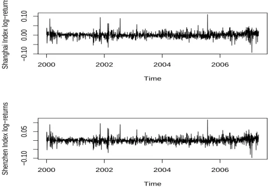
For the empirical work, the valuation scheme for the bivariate option under GARCH-GH model with dynamic copula outlined in Section 3 is applied to call-on-max option on the Shanghai Stock Composite Index and the Shenzhen Stock Composite Index. The sample contains 1857 daily observations from 4 January 2000 to 29 May 2007. The log-returns of Shanghai Stock Composite Index and Shenzhen Stock Composite In-dex are shown in Figure 1, it is noted that the outliers typically occur simultaneously and almost in the same direction.

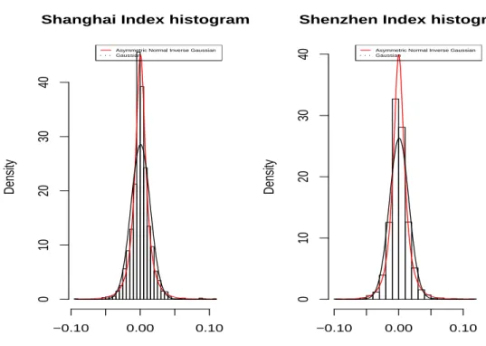
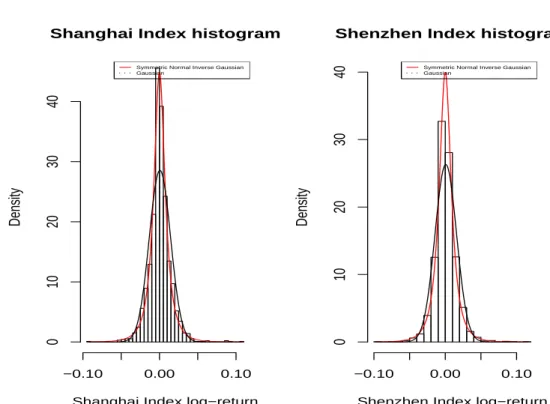
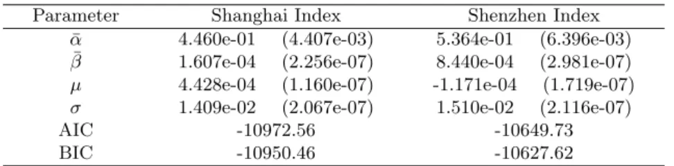
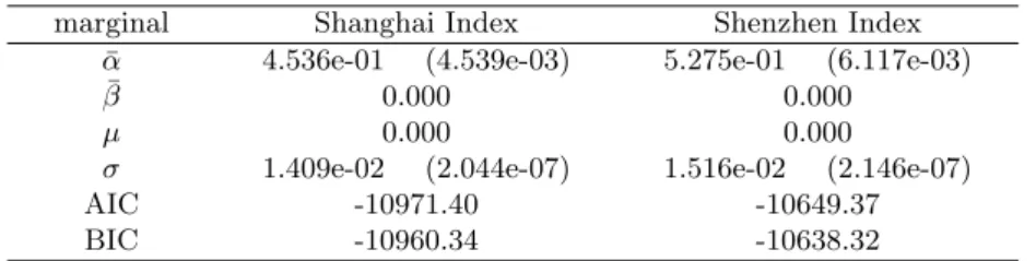
In this empirical work, we restrict the GH distribution to the NIG distri-bution which gives a better fit to our data set. The NIG fitting results are shown in Figure 2 and Table 1. The fitted NIG distributions are asymmet-ric. But simulation provides skewness parameter ¯β close to 0 and location parameter µ nearly equal to 0, thus in order to make the GARCH-NIG fitting more tractable, an assigned symmetric NIG distribution with 0

location is refitted and the results are shown in Figure 3, Figure 4 and Table 2.

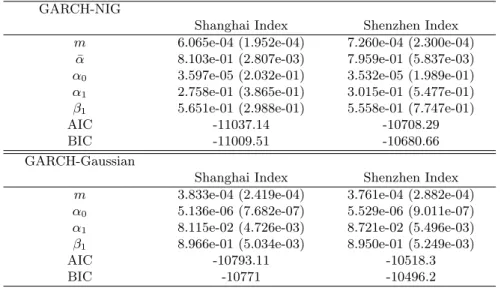
The parameter estimates for the GARCH (1,1) with symmetric NIG in-novation models for the underlying assets log-returns are listed in Table 3, and in order to compare, the results for GARCH-Gaussian model are also provided. From the AIC and BIC values of the two types of model, GARCH-NIG models appear better for both Shanghai Stock Composite Index and Shenzhen Stock Composite Index.

4.2 Dynamic copula method

Here, we consider the bivariate vector composed with the two assets. Sev-eral kinds of copulas are considered to describe the dependence structure between these assets on the whole period, including Gaussian, Frank, Gumbel, Clayton, Student t copulas JH97. All the copulas mentioned above are fitted to the support set of the standardized innovation pairs from GARCH-NIG and GARCH-Gaussian models respectively. The fit-ting results are listed in Table 4. AIC criterion is used to choose the best fitting copula. From the models fitted to the standardized innovations for Shanghai and Shenzhen stock composite indexes, the one which has the smallest AIC value is the Student t copula both for GARCH-NIG and GARCH-Gaussian models. Therefore, Student t copula is considered as the best fitting copula in case of static dependence for both models.

Using moving window allows to observe the change trend in a direct way, and makes the dynamics specification more reasonable corresponding to the real setting. Therefore, the whole sample is divided into subsamples separated by the moving window. 16 windows in which each consists of 300 observations are moved by 100 observations. Along with the moving of the window, series of best fitting copulas on different subsamples are decided by AIC criterion. The results for the best fitting copulas on all subsamples for GARCH-NIG and GARCH-Gaussian model are shown in Table 5. Results listed in Table 5 show that on almost all subsamples, Stu-dent t copula turns out to be the best fitting copula for the GARCH-NIG model. So it is rather reasonable to assume that for the GARCH-NIG model, the copula family remains static as Student t, while the param-eter changes along the time. As far as the GARCH-Gaussian model is concerned, the copula changes a lot. For the 2nd, 3rd and 5th windows,

although the Gaussian copula seems as the best fitting, the Student t cop-ula offers the very close AIC value (with the difference not bigger than 2). And for the 7th, 8th, 9th, 10th, 11th windows, the Frank copula provides the best fitting, and the Student t copula is the secondly best fitting. Thus we still assume that the copula family is static as the Student t but the parameters vary. In addition, it can be observed that the correlation does not change a lot for both GARCH-NIG and GARCH-Gaussian models while the degree of freedom varies obviously for both of the two models. Therefore, it seems reasonable to assume that the degree of freedom varies along time while the correlation remains static.

The time-varying function for the degree of freedom of the Student t copula is put forward as:

νt= l−1(s0+ s1ε1,t−1ε2,t−1+ s1l(νt−1)), (12)

where s0, s1, s2 are real parameters and l(·) is a function defined by

l(ν) = log( 1 ν_{− 2}),

to ensure that the degree of freedom is not smaller than 2. The corre-sponding estimate results for the dynamic copula parameter described in Equation (13) are listed in Table 6.

4.3 Pricing bivariate option

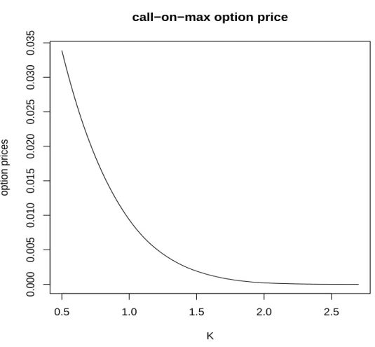
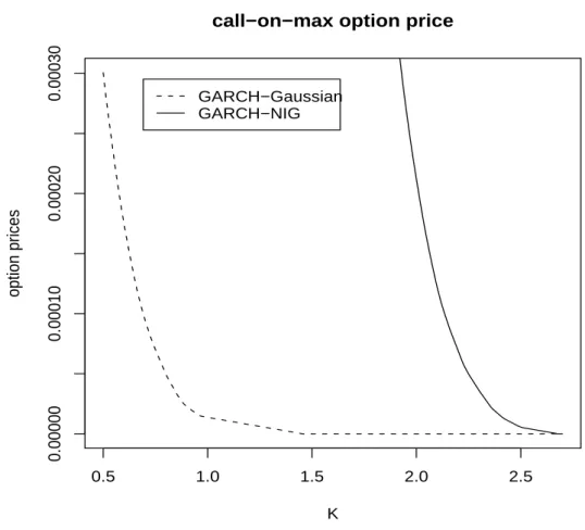
Standard normal random variables can then be generated from this con-ditional Student t copula with time-varying parameter, and according to two NIG margin distributions, log-return innovations can be sampled to compute the price of the option. Considering that the initial asset prices need to be close for the option to make sense, it is assumed here that they are normalized to unity. Different maturities can be considered, and 1 month (20 trading days) are displayed here just devoting itself to illus-trating the approach. Moreover, the strike price is set at levels between 0.5 and 2.7. The risk-free rate is assumed to be 6% per annum, and λ is considered as 5%. Using the proposed dynamic copula method with time-varying parameter, the option prices are represented in Figure 5. Compared with the option prices implied by the GARCH-Gaussian dy-namic model in Figure 6, it can be observed that the GARCH-Gaussian model generally underestimates the price.

The above pricing can be numerically assessed by repeating the following empirical Monte Carlo simulation steps:

1. Identify two observable two-dimensional sufficient statistics at time t, i.e., (ri,t, hi,t) for i = 1, 2;

2. Using the estimated results of the dynamic copula from the physical model, for each i = 1, 2, generate N standard Normal random numbers

Z_{i,T +1}j , j = 1,· · · , N in order to make an empirical adjustmnt. We first

compute the discounted sample average of simulated asset price for time t + 1, and then multiply each of the N simulated asset prices by the ratio of the initial asset price over the discounted average. This adjustment ensures that the simulated sample has an empirical martingale property;

3. Repeat steps 1 to 2 until arriving at N simulated asset prices, S_T(j), j = 1, . . . , N ;

4. Compute each of N option payoffs. Average N option payoffs, and discount the average, using the risk-free interest rate, back to the time of option valuation.

Our Monte Carlo study is based on N = 100, 000 replications, resulting in simulation errors in the order of magnitude of 1 basis point for 1 month maturity claims.

5 Conclusion

In this paper, a systematic new approach for bivariate option pricing un-der GARCH-GH model with dynamic copula has been introduced. The introduction of GARCH-GH model on each asset permits to take into account most of the stylized facts observed on the data set, see for recent development in CGI08. The risk neutral model permits to get an analyt-ical expression for the fair value of the call-on-max option.

Concerning the adjustment of the dynamic copula, we use fixed moving windows, this approach could be extended to use other lengths of win-dows: the question which arises will be the good criterion to retain the copula. Indeed using AIC criterion, we need to know whether a change in the value of this criterion is relevant or not, which is not an easy task. In this work, we observe stability concerning the adjustment of the Student t copula, with changing parameters, thus we keep static family and make varying the parameters.

Other extensions concern the choice of the type of GARCH process. For instance, the BL-GARCH SV03 could be interesting. Indeed this class of models permits to take into account explosion and clusters as stylized facts, DGW08.

Acknowledgment The authors want to thant the two referees for their precious remarks which permit to perform this paper.

Time

Shanghai Index log−returns −0.10 2000 2002 2004 2006

0.00

0.10

Time

Shenzhen Index log−returns 2000 2002 2004 2006

−0.10

0.05

Fig. 1. Log-returns for Shanghai Stock Composite Index and Shenzhen Stock Com-posite Index from 4 January 2000 to 29 May 2007

Shanghai Index histogram

Shanghai Index log−return

Density −0.10 0.00 0.10 0 10 20 30 40

Asymmetric Normal Inverse Gaussian Gaussian

Shenzhen Index histogram

Shenzhen Index log−return

Density −0.10 0.00 0.10 0 10 20 30

40 Asymmetric Normal Inverse Gaussian Gaussian

Fig. 2. Asymmetric NIG fitting for log-returns of Shanghai Stock Composite Index and Shenzhen Stock Composite Index

Shanghai Index histogram

Shanghai Index log−return

Density −0.10 0.00 0.10 0 10 20 30 40

Symmetric Normal Inverse Gaussian Gaussian

Shenzhen Index histogram

Shenzhen Index log−return

Density −0.10 0.00 0.10 0 10 20 30

40 Symmetric Normal Inverse Gaussian Gaussian

Fig. 3.Symmetric NIG fitting for log-returns of Shanghai Stock Composite Index and Shenzhen Stock Composite Index

−0.10 0.00 0.10

−0.05

0.00

0.05

NIG Q−Q plot for Shanghai

Sample quantiles

Theoretical quantiles

Symmetric Normal Inverse Gaussian Gaussian

−0.10 0.00 0.10

−0.05

0.00

0.05

NIG Q−Q plot for Shenzhen

Sample quantiles

Theoretical quantiles

Symmetric Normal Inverse Gaussian Gaussian

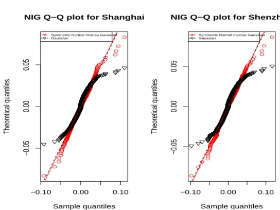
Fig. 4.Q-Q plots of symmetric NIG fitting for log-returns of Shanghai Stock Composite Index and Shenzhen Stock Composite Index

0.5 1.0 1.5 2.0 2.5 0.000 0.005 0.010 0.015 0.020 0.025 0.030 0.035

call−on−max option price

K

option prices

Fig. 5.1 month maturity call-on-max option prices as a function of the strike using the method of dynamic Student t copula with time-varying parameter

0.5 1.0 1.5 2.0 2.5

0.00000

0.00010

0.00020

0.00030

call−on−max option price

K

option prices

GARCH−Gaussian GARCH−NIG

Fig. 6. 1 month maturity call-on-max option prices as a function of the strike from GARCH-NIG and GARCH-Gaussian models with dynamic copula

Table 1.Estimates of asymmetric NIG fitting parameters for marginal log-returns

Parameter Shanghai Index Shenzhen Index ¯

α 4.460e-01 (4.407e-03) 5.364e-01 (6.396e-03) ¯

β 1.607e-04 (2.256e-07) 8.440e-04 (2.981e-07) µ 4.428e-04 (1.160e-07) -1.171e-04 (1.719e-07) σ 1.409e-02 (2.067e-07) 1.510e-02 (2.116e-07)

AIC -10972.56 -10649.73

BIC -10950.46 -10627.62

σ = δ ¯α/p ¯α2

−β¯2 is reparameterized as a dispersion parameter that can be seen as the volatility. Figures in brackets are standard errors.

Table 2.Estimates of symmetric NIG fitting parameters for marginal log-returns

marginal Shanghai Index Shenzhen Index ¯

α 4.536e-01 (4.539e-03) 5.275e-01 (6.117e-03) ¯

β 0.000 0.000

µ 0.000 0.000

σ 1.409e-02 (2.044e-07) 1.516e-02 (2.146e-07)

AIC -10971.40 -10649.37

BIC -10960.34 -10638.32

Table 3.Estimates of GARCH-NIG and GARCH-Gaussian parameters for marginal log-returns

GARCH-NIG

Shanghai Index Shenzhen Index m 6.065e-04 (1.952e-04) 7.260e-04 (2.300e-04)

¯

α 8.103e-01 (2.807e-03) 7.959e-01 (5.837e-03) α0 3.597e-05 (2.032e-01) 3.532e-05 (1.989e-01)

α1 2.758e-01 (3.865e-01) 3.015e-01 (5.477e-01)

β1 5.651e-01 (2.988e-01) 5.558e-01 (7.747e-01)

AIC -11037.14 -10708.29

BIC -11009.51 -10680.66

GARCH-Gaussian

Shanghai Index Shenzhen Index m 3.833e-04 (2.419e-04) 3.761e-04 (2.882e-04) α0 5.136e-06 (7.682e-07) 5.529e-06 (9.011e-07)

α1 8.115e-02 (4.726e-03) 8.721e-02 (5.496e-03)

β1 8.966e-01 (5.034e-03) 8.950e-01 (5.249e-03)

AIC -10793.11 -10518.3

BIC -10771 -10496.2

Table 4.Copula Fitting Results

GARCH-NIG

Copula Parameter AIC value

Gaussian 9.191e-01 (4.205e-02) -3517.934 Gumbel 3.732 (7.285e-02) -3460.264 Clayton 3.905 (1.051e-01) -2915.304 Frank 14.070 (3.242e-01) -3255.558 Student t 9.221e-01 (3.914e-02); 3.675 (2.119) -3683.532

GARCH-Gaussian

Copula Parameter AIC value

Gaussian 9.314e-01 (4.402e-02) -3757.412 Gumbel 3.971 (7.845e-02) -3528.21 Clayton 4.081 (1.114e-01) -2728.87 Frank 16.593 (3.611e-01) -3591.436 Student t 9.349e-01 (5.095e-02); 5.807 (1.601) -3797.926

Figures in brackets are standard errors and for Student t copula, the first parameter is the correlation, the second parameter is the degree of freedom.

Table 5.Dynamic Copula Analysis using Moving Window

GARCH-NIG GARCH-Gaussian

ith

Co Parameter Co Parameter

1 t 9.109e-1(1.032e-1); 2.444(1.302) Ga 9.308e-1(1.034e-1) 2 t 9.064e-1(9.990e-2); 3.084(9.590e-1) Ga 9.247e-1(1.036e-1) 3 t 9.308e-1(9.505e-2); 5.594(9.384e-1) Ga 9.381e-1(1.103e-1) 4 t 9.451e-1(1.157e-1) 3.903(1.017) t 9.539e-1(6.831e-2) 14.784(2.675) 5 t 9.602e-1(2.804e-1); 7.919(4.215) Ga 9.646e-1(1.437e-1) 6 t 9.697e-1(1.142e-1) 6.826(3.352) t 9.730e-1(1.164e-1) 15.262(5.337) 7 t 9.654e-1(1.442e-1); 8.098(3.385) Fr 25.157(1.293) 8 t 9.598e-1(9.931e-2); 6.005(2.104) Fr 22.866(1.193) 9 t 9.444e-1(2.117e-1); 7.087(3.630) Fr 18.971(1.003) 10 t 9.385e-1(1.594e-1); 7.675(2.000) Fr 18.115(9.655e-1) 11 t 9.419e-1(1.612e-1); 9.947(1.352) Fr 18.914(1.000) 12 Gu 4.450(2.167e-1) Gu 4.800(2.347e-1) 13 t 9.228e-1(1.533e-1); 5.682(2.388) Ga 9.371e-1(1.143e-1) 14 t 8.831e-1(2.594e-1); 3.574(10.030) Ga 9.062e-1(9.686e-2) 15 t 8.727e-1(7.247e-2) 3.300(8.206) t 9.009e-1(1.092e-1) 5.012(3.371e-1) 16 t 8.493e-1(1.030e-1) 4.937(2.129) t 8.765e-1(1.043e-1) 10.513(1.601) Figures in brackets are standard errors. “Co” represents “Copula type”, the short notes “t”, “Gu”, “Ga” and “Fr” represent respectively “Student t”, “Gumbel”, “Gaussian” and “Frank” copulas. And for the Student t copula, the first parameter is the correlation, the second parameter is the degree of freedom.

Table 6.Parameter estimates for dynamic Student t copula with time-varying param-eter

GARCH-NIG GARCH-Gaussian p 9.176e-01 (2.361e-02) 9.267e-01 (2.483e-02) s0 4.384e-01 (1.497) 1.065 (5.452e-03)

s1 -6.055e-02 (7.407e-01) 1.676e-01 (1.190e-03)

s2 -9.414e-01 (4.165e-01) -6.971e-01 (3.289e-02)

References

[Akaike(1974)] Akaike, H. 1974. A new look to the statistical model identification. IEEE Transactions on Automatic Control AC-19: 716-723.

[Barone-Adesi et al.(2004)] Barone-Adesi, G., Engle, R.F. and Mancini, L. 2004. Garch options in incomplete markets. Working Paper, NCCR-FinRisk.

[Black and Scholes(1973)] Black, F. and Scholes, M.S. 1973. The pricing of options and corporate liabilities. Journal of Political Economy 81: 637-654.

[Brennan(1979)] Brennan, M. 1979. The pricing of contingent claims in discrete time models. Journal of Finance 34: 53-68.

[Cherubini and Luciano(2002)] Cherubini, U. and Luciano, E. 2002. Bivariate option pricing with copulas. Applied Mathematical Finance 9: 69-86.

[Chorro et al. (2008)] Chorro, C., Gu´egan, D., Ielpo, F. 2008a. Option pricing under GARCH models with generalised hyperbolic innovations (I): Methodology. Working Paper, CES-Universit´e Paris 1, n 2008-37.

[Chorro et al. (2008)] Chorro, C., Gu´egan, D., Ielpo, F. 2008b. Option pricing under GARCH models with generalised hyperbolic innovations (I): data and Results. Work-ing Paper, CES-Universit´e Paris 1, n 2008-47.

[Christoffersen et al. (2006)] Christoffersen, S., Heston, S., Jacobs, K. 2006. Option valuation with conditional skewness. Journal of Econometrics 131: 253-284. [Cox(1975)] Cox, J. 1975. Notes on option pricing I: Constant elasticity of variance

diffusions. Working Paper, Stanford University.

[Dias and Embrechts(2003)] Dias, A. and Embrechts, P. 2003. Dynamic copula models for multivariate high-frequency data in finance. Working Paper, ETH Zurich. [Ding et al. (1993)] Ding, Z., Granger, C. W. J., Engle, R. F. 1993. A long memory

property of stock market returns and a new model. Journal of Empirical Finance 1: 83-106.

[Diongue et al. (2008)] Diongue, A. K., Gu´egan, D., Wolff, R. 2008. Likelihood esti-mation for the BL-GARCH model under elliptical distributed innovations. Working Paper, CES-Universit´e Paris 1.

[Duan(1995)] Duan, J.-C. 1995. The GARCH option pricing model. Mathematical Fi-nance5: 13-32.

[Duan(1996)] Duan, J.-C. 1996. Cracking the smile. RISK 9: 55-59.

[Duan(1999)] Duan, J.-C. 1999. Conditionally fat-tailed distributions and the volatility smile in options. Working Paper, University of Toronto.

[Eberlein and Keller(1995)] Eberlein, E. and Keller, U. 1995. Hyperbolic distributions in finance. Bernoulli 1: 281-299.

[Eberlein and Prause(2002)] Eberlein, E. and Prause, K. 2002. The generalized hyper-bolic model: financial derivatives and risk measures. Paper presented in Mathematical Finance-Bachelier Congress 2000, ed. H. Geman, D. Madan, S. Pliska and T. Vorst, 245-267. Springer Verlag.

[Elliott and Madan(1998)] Elliott R.J. and Madan D.B. 1998 A discrete Time equiv-alent martingale Measure, empMathematical finance 8: 127 - 152.

[Embrechts et al.(2002)] Embrechts, P., McNeil, A. and Strausmann, D. 2002. Corre-lation and dependence in risk management: properties and pitfalls. In Risk Man-agement: Value at Risk and Beyond, ed. M.A.H. Dempster, 176-223. Cambridge: Cambridge University Press.

[Engle(1982)] Engle, R. F. 1982. Autoregressive conditional heteroscedasticity with estimates of the variance of United Kingdom inflation. Econometrica 50: 987-1007.

[Forbes and Rigobon(2002)] Forbes, K. and Rigobon, R. 2002. No contagion, only in-terdependence: Measuring stock market co-movements. Journal of Finance 57: 2223-2261.

[Gerber and Shiu(1994)] Gerber H.U. and Shiu S.W. 1994 Option pricing by Esscher Transforms, Transaction of Society of Actuaries 20-22:, 659 - 689.

[Geske(1979)] Geske, R. 1979. The valuation of compound options. Journal of Finan-cial Economics7: 63-81.

[Glosten et al. (1993)] Glosten, L.R., Jagannathan, R. and Runkle, D.E. 1993. On the relation between the expected value and the volatility of the Nominal excess return on stocks . Journal of Finance 48: 1779C1801.

[Gourieroux and Monfort(2007)] Gourieroux C. and Monfort A. 2007. Econometric specifications of stochastic discount Factor Models, Journal of Econometrics 136: 509 - 530.

[Granger et al.(2006)] Granger, C.W.J., Ter¨asvirta, T. and Patton, A.J. 2006. Com-mon factors in conditional distributions for bivariate time series. Journal of Econo-metrics 132: 43-57.

[Gu´egan and Caillault(2007)] Gu´egan, D. and Caillault, C. 2007. Forecasting VaR and Expected Shortfall using Dynamical Systems: A Risk Management Strategy, to ap-pear in Frontiers in Finance.

[Gu´egan and Zhang(2006)] Gu´egan, D. and Zhang, J. 2006. Change analysis of dy-namic copula for measuring dependence in multivariate financial data. To appear in Quantitative Finance.

[Heston and Nandi(2000)] Heston, S. and Nandi, S. 2000. A closed-form GARCH op-tion pricing model. The Review of Financial Studies 13: 586-625.

[Heynen et al.(1994)] Heynen, R., Kemna, A. and Vorst, T. 1994. Analysis of the term structure of implied volatilities. Journal of Financial and Quantitative 29: 31-56. [Hull and White(1987)] Hull, J. and White, A. 1987. The pricing of options on assets

with stochastic volatilities. Journal of Finance 42: 281-300.

[Jensen and Lunde(2001)] Jensen, M. B. and Lunde, A. 2001. The NIG-S&ARCH model: a fat-tailed, stochastic, and autoregressive conditional heteroskedastic volatil-ity model. Econometrics Journal 4: 319-342.

[Joe(1997)] Joe, H. 1997. Multivariate Models and Dependence Concepts. Chapman & Hall, London.

[Johnson(1987)] Johnson, H. 1987. Options on the maximum or the minimum of several assets. Journal of Financial and Quantitative Analysis 22: 277-283.

[Jondeau and Rockinger(2004)] Jondeau, E. and Rockinger, M. 2004. Conditional de-pendency of financial series: the copula-GARCH model. Journal of Money and Fi-nance, forthcoming.

[Margrabe(1978)] Margrabe, W. 1978. The value of an option to exchange one asset for another. Journal of Finance 33: 177-186.

[Merton(1973)] Merton, R. 1973. The theory of rational option pricing. Bell Journal of Economics and Management Science 4: 141-183.

[Merton(1976)] Merton, R. 1976. Option pricing when underlying stock returns are discontinuous. Journal of Financial Economics 3: 125-144.

[Nelson(1991)] Nelsen, D.B. 1991. Conditional heteroskedasticity in asset returns: A new approach. Econometrica 59: 347-370.

[Nelsen(1999)] Nelsen, R. 1999. An introduction to copulas. Lecture Notes in Statistics No. 139. Springer, New York.

[Patton (2006)] Patton, A. J. 2006. Modelling Asymmetric Exchange Rate Depen-dence. International Economic Review 47: 527-556.

[Reiner (1992)] Reiner, E. 1992. Quanto mechanics. From Black-Scholes to Black Holes: New Frontiers in Options. Risk Books London: 147-154.

[Rosenberg (1999)] Rosenberg, J.V. 1999. Semiparametric pricing of multivariate con-tingent claims. Working Paper S-99-35, Stern School of Business, New York Univer-sity, New York.

[Rubinstein (1976)] Rubinstein, M. 1976. The valuation of uncertain income streams and the pricing of options. Bell Journal of Economics and Management Science 7: 407-425.

[Rubinstein (1983)] Rubinstein, M. 1983. Displaced diffusion option pricing. Journal of Finance 38: 213-217.

[Shimko(1994)] Shimko, D.C. 1994. Options on futures spreads: Hedging, speculation, and valuation. Journal of Futures Markets 14: 183-213.

[Sklar(1959)] Sklar, A. 1959. Fonctions de r´epartition `a n dimensions et leurs marges. Publications de l’Institut de Statistique de L’Universit´e de Paris8: 229-231. [Stentoft (2006)] Stentoft, L. 2006. Modelling the volatility of financial asset returns

using the Normal Inverse Gaussian distribution: With an application to option pric-ing. Working Paper, Department of Economics, University of Aarhus, Denmark. [Storti and Vitale(2003)] Storti, G. and Vitale C. 2003. BL-GARCH models and

asym-metries in volatility. Statistical Methods and Applications 12: 19-39.

[Stulz(1982)] Stulz, R.M. 1982. Options on the minimum or the maximum of two risky assets: analysis and applications. Journal of Financial Economics 10: 161-185. [Umberto et al. (2004)] Umberto, C., Elisa, L., Walter, V. 2004. Copula Methods in

Finance. J. Wiley & Jons, Inc.

[Van den Goorbergh et al. (2005)] Van den Goorbergh, R.W.J., Genest, C., Werker, B.J.M. 2005. Bivariate option pricing using dynamic copula models. Insurance: Math-ematics and Economics 37: 101C114.

Annex: A short introduction for copulasJH97,NR99

Let X = (Xn)n∈Z = {(Xi1, Xi2, . . . , Xid) : i = 1, 2, . . . , n} be a

d-dimension random sample of n multivariate observations from the un-known multivariate distribution function F (x1, x2, . . . , xd) with

continu-ous marginal distributions F1, F2, . . . , Fd. The characterization theorem

of SA59 implies that there exists a unique copula Cθ such that

F (x1, x2, . . . , xd) = Cθ(F1(x1), F2(x2),· · · , Fd(xd))

for all x1, x2, . . . , xd ∈ R. Conversely, for any marginal distributions

F1, F2, . . . , Fdand any copula function Cθ, the function Cθ(F1(x1), F2(x2), . . . , Fd(xd))

is a multivariate distribution function with given marginal distributions F1, F2, . . . , Fd. This theorem provides the theoretical foundation for the

widespread use of the copula approach in generating multivariate distri-butions from univariate distridistri-butions.

In order to adjust a copula Cθ on a set of process, we will use maximum

likelihood method and AIC criterion [][]AH74. Details can be found in UEW04.

.1 Gaussian copula

The copula of the d-variate normal distribution with linear correlation matrix R is

CGa_R (u) = Φd_R(Φ−1(u1), Φ−1(u2),· · · , Φ−1(ud)),

where Φd_Rdenotes the joint distribution function of the d-variate standard normal distribution function with linear correlation matrix R, and Φ−1 denotes the inverse of the distribution function of the univariate standard Gaussian distribution. Copulas of the above form are called Gaussian cop-ulas. In the bivariate case, we denote ρ as the linear correlation coefficient, then the copula’s expression can be written as

CGa(u, v) = Z Φ−1_(u) −∞ Z Φ−1_(v) −∞ 1 2π(1_{− ρ}2₎1/2exp{− s2_{− 2ρst + t}2 2(1_{− ρ}2₎ }dsdt.

The Gaussian copula CGa with ρ < 1 has neither upper tail dependence nor lower tail dependence.

.2 Student-t copula

If X has the stochastic representation

X= µ +d √

ν √

SZ, (13)

where = represents the equality in distribution or stochastic equality,d µ ∈ Rd_{, S ∼ χ}2

ν and Z ∼ Nd(0, Σ) are independent, then X has a

d-variate tν distribution with mean µ (for ν > 1) and covariance matrix ν

ν−2Σ (for ν > 2). If ν ≤ 2 then Cov(X) is not defined. In this case we

just interpret Σ as the shape parameter of the distribution of X. The copula of X given by Equation (13) can be written as

C_ν,Rt (u) = td_ν,R(t−1

ν (u1), t−ν1(u2),· · · , t−ν1(ud)),

where Rij = Σij/pΣiiΣjj for i, j ∈ {1, 2, · · · , d}, td_ν,R denotes the

dis-tribution function of √νY/√S, S ∼ χ2

ν and Y ∼Nd(0, R) are

indepen-dent. Here tν denotes the margins of td_ν,R, i.e., the distribution function

of √νYi/

√

S for i = 1, 2,_{· · · , d. In the bivariate case with the linear} cor-relation coefficient ρ, the copula’s expression can be written as

C_ν,Rt (u, v) = Z t−1ν (u) −∞ Z t−1ν (v) −∞ 1 2π(1_{− ρ}2₎1/2{1+ s2_{− 2ρst + t}2 ν(1− ρ2₎ } −(ν+2)/2_dsdt.

Note that ν > 2. And the upper tail dependence and the lower tail de-pendence for Student t copula have the equal value.