HAL Id: hal-02428709
https://hal.archives-ouvertes.fr/hal-02428709
Preprint submitted on 6 Jan 2020
HAL is a multi-disciplinary open access
archive for the deposit and dissemination of sci-entific research documents, whether they are pub-lished or not. The documents may come from teaching and research institutions in France or abroad, or from public or private research centers.
L’archive ouverte pluridisciplinaire HAL, est destinée au dépôt et à la diffusion de documents scientifiques de niveau recherche, publiés ou non, émanant des établissements d’enseignement et de recherche français ou étrangers, des laboratoires publics ou privés.
Distributed under a Creative Commons Attribution - NonCommercial| 4.0 International License
To cite this version:
Helmstetter Andrew J., Tom Van Dooren. Determinants of growth and body size in Austrolebias South-American annual killifish. 2020. �hal-02428709�
1
Determinants of growth and body size in Austrolebias South-American annual killifish 1
2
Andrew Helmstetter1,2
3
Tom JM Van Dooren3
4
1
Department of Life Sciences, Silwood Park Campus, Imperial College London, Ascot, SL5 5 7PY, 5
Berkshire, UK 6
2CNRS - UMR DIADE, University of Montpellier, Montpellier, France
7 8
3CNRS - UMR 7618 Institute of Ecology and Environmental Sciences (iEES) Paris, Sorbonne
9
University, Case 237, 4 place Jussieu, 75005 Paris, France 10 11 Version 31 December 2019 12 13 Words: 6151 14 Figures: 5 15 Tables: 1 16
The data will be deposited in the Dryad Digital Repository. 17
2 Abstract (190)
19
Patterns of size variation in fish are supposed to be generated by growth differences, not by egg or 20
hatchling size variation. However, annual killifish live in temporary ponds with a limited time period 21
available for growth and reproduction. It has therefore been hypothesized that among annual 22
killifish, hatchling size variation should be of large relative importance to generate adaptive adult 23
size variation. Using growth curves of 203 individuals from 18 Austrolebias species raised in a 24
common environment, we demonstrate that hatchling size variation indeed is a main determinant of 25
adult size variation in annual killifish, in agreement with the time constraint hypothesis. 26
Furthermore, we find an increased early growth rate in piscivorous species augmenting their 27
difference in size from small congeneric species. This should be adaptive if size differences 28
determine predation success. Environmental effects of spatial location of the population of origin on 29
hatchling size and growth suggest that the time constraint might be weakened in populations 30
occurring near the Atlantic coast. Our study reveals how extreme environments demand specific life 31
history solutions to achieve adaptive size variation and that there might be scope for local 32
adaptations in growth trajectories. 33
3 Introduction
35
36
Body size differences are seen as key to understanding life history variation (Roff 1993). Teleost fish 37
alone are spanning nearly nine orders of magnitude in mature size and this is supposed to be due to 38
evolved differences in growth, not to size variation at hatching (Sibly et al 2015). At the same time, 39
there is enormous variation in life cycles among teleost fish and in the ecological and evolutionary 40
variability affecting size differences between closely related species and between and within 41
populations (Hutchings 2002). For example, Atlantic salmon vary 14-fold in size at maturity between 42
populations (Hutchings and Jones 1998) and this variability has been linked to temperature-43
dependent growth (Jonsson et al 2013). 44
Size variation and adaptation in fish is much studied in the context of size-selective harvesting (Law 45
2007). The topic has spurred a modelling effort to support arguments that responses of populations 46
to size-selective harvesting are adaptive (Ernande et al. 2004). Other modelling studies have aimed 47
to predict how competition can affect the emergence of size differences within populations or 48
between species. For example, Persson et al (2000) and Claessen et al (2000) have shown that 49
significant size differences can emerge within fish populations as a consequence of competition for 50
food and cannibalism, leading to so-called dwarfs and giants. Van Dooren et al. (2018) referred to 51
these studies to propose that large piscivorous annual killifish and their prey evolved in sympatry 52
due to a similar scenario of adaptation. Metabolic scaling studies such as Sibly et al (2015) then state 53
that such size differences between fish species must be due to slower or faster juvenile growth, 54
whereas all individuals within a species should grow as fast as environmental conditions for 55
development and metabolism permit. This theory implies that size differences within and between 56
populations can then only be explained by different environmental conditions which individuals 57
experience, leaving little or no room for adaptive variation in the use of resources to achieve 58
particular body sizes. On top of that, expected relative growth rates in fish are expected to decrease 59
4
with age (Pauly 1979) such that initial growth differences and initial environments have larger 60
effects on adult size. 61
62
Within the toothcarps (Cyprinodontiformes), annual killifish have evolved at least five times from 63
non-annual species (Furness et al 2015, Helmstetter et al 2016). Annualism denotes that these 64
species inhabit ephemeral waters and that their life history strategy resembles that of annual plants: 65
they establish egg banks where embryos survive dry periods by going through one or several 66
diapauses during development (Wourms 1972). Large size differences among closely related annual 67
killifish species have evolved repeatedly (Costa 2011). Within the genus Austrolebias which occurs in 68
South-American temperate environments, large size evolved from small (Van Dooren et al 2018, 69
Helmstetter et al. 2018) and adult body lengths range from about three centimeter to fifteen (Costa 70
2006), corresponding to a more than hundredfold difference in volume. One of the clades with large 71
species in Austrolebias have become specialized piscivores (Costa 2011, Van Dooren et al 2018). In 72
the African genus Nothobranchius there is similar size variation involving the evolution of piscivory 73
(Costa 2011, Costa 2018). This genus is well-known for its explosive growth and extremely early 74
maturity, observed both in the lab and the field (Blažek et al 2013, Vrtilek et al 2018). Within killifish, 75
adult body sizes are not only determined by growth variability as Sibly et al (2015) predicted. 76
Eckerström‐Liedholm et al. (2017) found that egg sizes in annual fish are larger than in non-annual 77
toothcarp species and explained this as an adaptation to environments with time constraints on 78
growth periods such as the temporary ponds annual fish inhabit. By being born from larger eggs, 79
annual killifish achieve large (adaptive) sizes by increasing hatchling size instead of growing longer. 80
We investigated in a common garden lab context and using the South-American annual killifish 81
genus Austrolebias how both small and large species in this genus achieve the size differences 82
known from the field and the lab (Figure one). We aimed to identify the major axis among different 83
components contributing to size variation (Schluter 1996): either growth variation (Sibly et al 2015) 84
5
or hatchling size variation (Eckerström‐Liedholm et al 2017) might explain body size differences 85
more. Hatchlings were obtained from a range of eighteen species mostly occurring in regions close 86
to the Atlantic Ocean and these were raised individually in separate tanks to provide individual 87
growth data. Sizes were measured repeatedly over an eight weeks period. We investigated effects of 88
different environmental variables on hatchling size and growth and compared the patterns of 89
growth rates between the geographic locations of the sites of origin of the populations in our study. 90
We find that hatchling size variation makes the largest contribution to size variation between 91
species, but the relative importance of early post-hatching growth on individual size variation is 92
comparable with hatchling size. Our results thus confirm that large body sizes in some species are to 93
a large extent determined by large hatchling size and we reject the hypothesis that only growth 94
variation matters for size differences between fish species. 95
96
Material and methods 97
98
We triggered hatching of embryos of 18 Austrolebias species (Fig. 1) stored in brown peat, by 99
flooding the peat and eggs with water (15 C, 20% aged tap water, 80% RO water, peat extract). Six of 100
the species are usually classified as large and they belong to three different clades (Van Dooren et al 101
2018, Helmstetter et al 2018). Three species in this experiment are from a single clade of large 102
species containing specialized piscivores (Costa 2010). The 18 species originate from three different 103
Atlantic coastal areas of endemism (Costa 2009), with the populations in this experiment originating 104
from a single such area per species (La Plata river basin, Negro river basin, Patos coastal lagoons, 105
Helmstetter et al. 2018). In these regions, temporary ponds dry in summer. The inland seasonal 106
pattern of rainfall in the Chaco region is different. At the moment of hatching, embryos were 107
between four and forty-two months old. 108
6 109
Hatchlings that were swimming freely (with inflated swim bladder) were placed in separate 0.25 L 110
plastic raising tanks and gradually moved into increasingly larger tanks as they grew. Water 111
parameters were controlled to the following values: <12 dGH, <10 mg/L NO3, < 0.1 mg/L NO2, < 0.25 112
mg/L NH3, pH = 7.0 - 8.0, 22 ± 0.5 C, by diluting water in the raising tanks daily with water from 113
reserves stored in the same room. The fish experienced a 14L:10D photoperiod. Hatchlings were fed 114
Artemia salina nauplii daily for two weeks and then a combination of Artemia salina, Chironomid
115
larvae, Tubifex and Daphnia pulex. We ensured that the raising tanks always contained live food, 116
such that the fish could feed to satiation. Each tank contained plants (Vesicularia dubyana and 117
Egeria densa) as well as 5 g of boiled brown peat to aggregate waste and maintain water
118
parameters. At day 58, 32 fish showed visible evidence of stunting or hampered growth (bent spine - 119
extreme lack of growth) and they were assigned to a separate "stunted" category for analysis. 120
121
Photography 122
We photographed individual fish using a digital USB microscope at hatching (day 1) and repeatedly 123
after that, after intervals of increasing duration with age. We obtained up to nine measurements per 124
individual fish. We constrained the fish in small chambers and photographed from a lateral and 125
dorsal perspective or placed larger fish in a shallow water layer in a petri dish to make lateral 126
pictures only. We measured total length, the distance from anterior tip of the maxilla to the 127
posterior tip of the caudal fin, using ImageJ. 128
129
Statistical analysis 130
Van Dooren et al (2018) and Helmstetter et al (2018) investigated whether shifts in selection regimes 131
occurred for size and niche traits within Austrolebias. Helmstetter et al (2018) identified a shift to a 132
7
selection regime with an increased optimum size for the clade containing A. elongatus. An analysis 133
for shifts on the posterior distributions of phylogenies in Van Dooren et al (2018) found similar shifts 134
for the other clades containing large species in a fraction of trees. Niche traits showed weak 135
evidence for a niche shift in the Negro area (Helmstetter et al 2018). These results make it necessary 136
to use membership of the clades with large species and the areas of endemism as explanatory 137
variables to accommodate effects of the detected regime shifts and to accommodate other similar 138
potential shifts for the traits we investigate. The remaining species differences are then random with 139
respect to these estimated shifts and the species effects can be treated as random effects. 140
141
Survival and stunting. Next to species differences in mortality, the incidence of stunted body
142
morphologies can indicate whether the environmental conditions we imposed permit normal 143
growth. We therefore assessed survival variation between species and whether the risk of becoming 144
stunted differed between species or depended on age of the embryos at inundation. The proportion 145
of individuals alive at day 50 (before some A. wolterstorfii were moved out of the experiment into 146
bigger tanks) was analysed using a binomial generalized additive (GAM, Wood 2017) or generalized 147
linear model (GLM cCullagh and Nelder 1989). Age at hatching, membership of a clade of large 148
species (yielding three categories of large species and one small), area of endemism per species 149
(three areas) and spatial coordinates of the location where the individuals were sampled that the 150
hatchling descended from were used as explanatory variables. 151
We used scores of the two components of a principal component PC analysis carried out on latitude 152
and longitude of all ponds. The ponds are not randomly distributed across the South-American 153
continent and we wanted to use two independent explanatory variables characterizing spatial 154
locations. The scores were standardized across all observations, so that their averages would be zero 155
across each dataset analysed. We first added scores as thin plate regression splines, hence GAM 156
were fitted (Wood 2017). When model comparisons revealed that these effects should not be 157
8
retained in the model or when they could all be fitted as linear effects, GLM's were fitted. Model 158
selection occurred by model simplification using likelihood ratio tests (LRT smooth terms and 159
interaction terms first if present) for comparisons. The probability to become stunted in the 160
experiment was analyzed similarly. We did not include sex effects (male/female/unknown) as an 161
explanatory variable here, as an individual might end up in the “unknown” category due to stunting 162
or premature death. 163
164
Initial size. We investigated variables affecting initial size at hatching using phylogenetic linear mixed
165
models (de Villemereuil and Nakagawa 2014) and linear mixed models (Pinheiro and Bates 2000). In 166
this manner, unbalanced data can be analyzed while different sources of variation in the data are 167
addressed simultaneously. In each model, we fitted different explanatory (fixed) variables, i.e., 168
embryo age, being classified as stunted, sex, areas of endemism, clades with large species and, as 169
above, we fitted models with the coordinate scores of capture locations. Different random effects 170
were included. In the maximal models, a random species effect with species covariances calculated 171
according the expected values under a Brownian motion model of evolution and next to that a 172
species effect with zero covariances. The expected covariances of the phylogenetic random effects 173
were calculated on the basis of a consensus nDNA tree from Helmstetter et al. (2018). We tested 174
whether including the phylogenetically structured random species effects contributed significantly 175
using a likelihood ratio test. We carried out model selection on the fixed effects as above using 176
likelihood ratio tests (Bolker et al 2009). We used function lmekin() to fit the mixed models including 177
phylogenetic random effects in R (Therneau 2012). For models which did not account for 178
phylogenetic relatedness, we used linear mixed models or generalized additive mixed models 179
(GAMM) with smooth functions to fit the scores of spatial coordinates. 180
9
Growth. We inspected growth curves y(t) of age t (days since hatching) using smooth functions
182
(Wood 2017), where we used thin plate regression splines of t per species and a smoothness 183
parameter shared between species (factor smooth interaction, function gam from library mgcv(), 184
option "bs=fs", Wood 2017). We found recent field data on individual size at age for three 185
Austrolebias species (Garcia et al 2018) and added these to a figure to check that our common
186
garden environment allowed individuals to grow to sizes comparable to field conditions. From two 187
lab studies, average sizes at different ages were extracted. Errea and Danulat (2001) provided an 188
average total length at age for Austrolebias viarius kept in the lab at 25C and Fonseca et al (2013) 189
provide average standard lengths for Austrolebias wolterstorffi kept at 24C. 190
Per individual, we calculated estimates of relative growth per day gi from the data as
191 192 𝑔𝑖= (𝑦𝑖+1 𝑦𝑖 ) 1 𝑡𝑖+1−𝑡𝑖 (Eqn. 1) 193 194
where yi and yi + 1 are successive size measurements on the same individual at ages ti and ti + 1. The
195
standard calculation of relative growth rate is the logarithm of this quantity (Hoffmann and Poorter 196
2002). We decided to integrate the instantaneous rate over a time interval of one day such that gi
197
becomes the relative increase per day which is easier to interpret. 100*(gi - 1) is the percentage
198
relative increase per day. We inspect and analyze relative increases per day at interval midpoints 199
𝑥𝑖 = (𝑡𝑖 + 𝑡𝑖+1 )/2. For illustration, we fitted smooth functions to the relative growth gi evaluated
200
at interval midpoints xi.
201
202
We investigated which variables affect relative growth as above, using generalized additive and 203
phylogenetic or non-phylogenetic mixed models. As each analysis contains several measures of 204
relative growth per individual, we added individual random effects nested within the non-205
phylogenetic species effect. We derived an expression for the error of the relative growth 206
10
calculations (Supplement), which we implemented in the mixed models. However, it was 207
systematically outperformed by a variance regression for the residual variance which changed with 208
the number of days after hatching (using varExp() weights in lme(), see Pinheiro and Bates 2000). 209
210
Relative contributions of initial size and relative growth to final size variation. Final size at the end
211
of the experiment (day 58 after hatching) depends on initial size at hatching and on the cumulative 212
growth over the time interval. We can partition cumulative growth into the contributions of 213
different periods to assess their relative importance in the generation of size variation. Log-214
transformed final size in the experiment consists of additive effects of initial size and growth as 215
shown below. This allows a useful variance decomposition (Rees et al 2010) of final size in the 216
experiment in terms of initial size and growth in different time intervals. 217
Because day 57 was the last day where the majority of fish were measured, we decomposed final 218
size of an individual 𝑦57 at day 57 of the experiment as follows:
219 𝑦57= 𝑦1𝑔⏞ 1𝑔2. . . 𝑔𝑛 𝐺𝑛 𝑔𝑛+1𝑔𝑛+2. . . 𝑔56 ⏞ 𝐺56 (Eqn. 2) 220 221
We chose to partition the relative growth per day gi into two periods, from day one to n and from day
222
n + 1 to day 56. For the analysis presented, we chose n = 28 because this provided two intervals of
223
similar length, with a large number of individuals measured at the end of the first interval. When we 224
log-transform (Eqn. 2), we obtain a sum of contributions to log final size: ln 𝑦57= 𝑙𝑛 𝑦1+ 𝑙𝑛 𝐺28+
225
𝑙𝑛 𝐺56. By means of a variance decomposition of ln 𝑦57 in the variances and covariances of these three 226
terms, we can assess the contribution of each term to final size variation in the experiment (Rees et 227
al. 2010). 228
For individuals that were not measured on days 29 and 57 but just before or after (14/111 and 14/94, 229
respectively), we extrapolated their sizes to these days (one or two days away), using the relative 230
11
growth over the last interval in the period. Magnitudes of the three contributions to final size in the 231
experiment were compared with paired samples Wilcoxon tests (Wilcoxon 1945). 232
The log size variance on day 57 of the experiment depends on the variances of the three components 233
contributing and their covariances (Eqn. 3). 234 235 𝜎2𝑙𝑛 𝑦57 = 𝜎2𝑙𝑛 𝑦1+ 𝜎2𝑙𝑛 𝐺28+ 𝜎2𝑙𝑛 𝐺56+ 2𝜎𝑙𝑛 𝑦1,𝑙𝑛 𝐺28+ 2𝜎𝑙𝑛 𝑦1,𝑙𝑛 𝐺56+ 2𝜎𝑙𝑛 𝐺28,𝑙𝑛 𝐺56 236 (Eqn. 3) 237 238
This is the covariance of final size with itself, which is the sum of the covariance of final size with initial 239
size, the covariance of final size with log relative growth until day 29 (early growth), and with log 240
relative growth between days 28 and 57 (late growth). We can interpret absolute values of these three 241
quantities divided by their sum as relative importances (Rees et al. 2010). 242
We determined relative importances of the three components for the variance between individuals, 243
restricted to individuals that were not stunted and which provided values for all three terms. We 244
resampled the dataset 100 times to obtain standard deviations on the relative importances. 245
We also calculated relative importances for the variance in final size between species. To obtain 246
estimates of component variances and covariances, we fitted multivariate mixed models (Bates et al 247
2014) to the three log components of final size with random species effects, allowing random effect 248
covariances between the three component traits and including the fixed effects listed above with 249
component-specific values. In agreement with the analyses of initial size and relative growth rates, we 250
present results assuming random effects per trait which are independent between species. The 251
covariances between the final sizes per species and each size component were then calculated as 252
follows. Predicted values of the summed fixed and random effect part of the mixed model were 253
generated for all species (twelve) where predictions for all three components could be made, To 254
remove individual variation in the fixed effects, we assumed for the predicted values that fish were 255
hatched after four months in the egg, did not show stunted growth and were sexed as a male. The 256
12
species-specific areas of endemism and taxa with large species were kept as fixed effects. The 257
variances and covariances of the predicted species values were calculated and a parametric bootstrap 258
of the mixed model was used to obtain standard deviations on the relative importances. Magnitudes 259
of the three predicted species contributions to final size were compared with paired samples Wilcoxon 260
tests (Wilcoxon 1945). 261
262
Comparison with other toothcarps. We compare our results with growth data from other studies on
263
annual and non-annual killifish. We found group averages of size at age, from which we calculated 264
relative growth per day as above. We point out that such estimates based on averages can be biased 265
(Hoffmann and Poorter 2002). We did not observe large changes in variances between pairs of data 266
points from which we calculated growth, therefore we expect such bias to be limited. We retrieved 267
data from studies on Austrolebias, Nothobranchius and non-annual rivulids and present relative 268
growth estimates we found or calculated. We have added relative growth on one Profundulid for 269
comparison, Fundulus heteroclitus, which is a non-annual killifish and a model organism (Schartl 270
2014). The data file is available as supplementary information. We present a graphical comparison of 271
the results from our experiment with the values obtained from these studies. 272
273
Results 274
275
We hatched 203 fish that could swim freely, of which 116 reached day 50 after hatching. The 276
principal component analysis on the coordinates of pond locations resulted in a first PC parallel with 277
the Atlantic coast in a North-South direction and a second PC orthogonal to that, which therefore 278
captures differences in the distance from the Atlantic Ocean. 279
13
Survival and stunting. When we plotted a log survivorship curve of all survival data, we noted that
281
the overall death rate is constant. We found no significant effects of age of the embryos on survival 282
probability until day 50. Species from the (A. robustus, A. vazferreirai) clade of large species have a 283
reduced survival probability ( = -2.06 (0.70), 2(1) = 10.50, p = 0.0012). At the same time, there is an
284
effect of the areas of endemism (2(2) = 9.81, p = 0.007). Species from the La Plata area of endemism
285
have a larger survival probability (estimate difference = 1.37 (0.50), Patos = 0.45 (0.45)). We 286
found a significant effect of area of endemism on the probability to become stunted (2(2) = 16.26, p
287
= 0.0002). There are no stunted individuals among species from the Negro area and about 20% in 288
species from the other two areas. Large species from the A. elongatus, A. prognathus, A. 289
cheradophilus group had an increased probability to become stunted ( = 1.57 (s.e. 0.43), 2(1) =
290
13.74, p = 0.0002). Smooth functions of spatial coordinate scores had no significant effects on 291
survival nor stunting. 292
293
Initial size. In GAMM models with all fixed and a random species effect, PC's of spatial coordinates
294
were best fitted with linear functions. We therefore fitted phylogenetic mixed models with such 295
linear functions to find that the phylogenetic random effect could be removed (LRT non-significant, 296
AIC smaller without phylogenetic covariances, Akaike 1974). From model selection of the fixed 297
effects, we found that the three taxa with large species systematically have larger hatchling sizes. 298
Embryos born from older eggs are larger (Table 1), demonstrating scope for cohort effects and 299
selection on size in the egg bank. Hatchlings of small species from the Patos area of endemism are 300
larger relative to the Negro area, and those from La Plata smaller. The first PC score, which increases 301
in a direction parallel to the Atlantic coast and to the North (called "North" from here on) does not 302
have a significant effect on hatchling size. The second PC increases towards the Atlantic Coast (Called 303
"Coast" from here on) and has a negative effect, hence hatchling size decreases for population 304
situated closer to the Atlantic Coast (Table 1). 305
14
Relative growth. Figure 2 shows growth curves for all individuals in the experiment, and fitted
306
smooth growth curve functions. The figure shows that relative to other studies and to field data, 307
individuals in our lab environment have similar or larger sizes for their ages. Moreover, in our 308
experiment fish seem slightly larger than in the field for their age. The growth data we collected is 309
therefore relevant. Moreover, individuals growing somewhat slower in our experiment are still 310
achieving sizes comparable to individuals in the field. Figure 3 shows the pattern of relative growth 311
across species. Most species initially increase in total length by about 5% per day and by the end of 312
the experiment, they still do so by about 2% per day on average. Fig. 3 shows that there is much 313
more individual variation around the species-specific averages for the first days after hatching. We 314
therefore analyzed daily relative growth until day 15 after hatching and after day 15 separately, thus 315
separating the dataset into two subsets with comparable numbers of intervals per individual. 316
Different factors affect species differences in different stages of growth (Table 1). Regarding growth 317
during the first fifteen days, a model with phylogenetic random effects did not outperform a model 318
with independent species effects (AIC -2495 vs. -2497, no difference in log-likelihood of the fitted 319
models). Table 1 thus presents a model with independent species effects. Species from the clade 320
containing Austrolebias elongatus grow more rapidly than the other species, about 1-2 % faster per 321
day. Individuals that could not be sexed by the end of the experiment were growing slower shortly 322
after hatching (Table 1). When splines of the PC's of spatial locations were fitted, these contributed 323
significantly in the complete model, but did not do so after model selection. 324
325
15
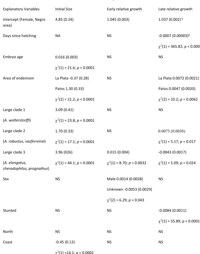
Table 1. Contributions of explanatory variables to hatchling size and relative growth variation. Parameter
327
estimates and their s.d. for fixed effects of the mixed effect models. Most model parameters are differences
328
from the estimated intercept, which predicts the value of an individual female of a small species originating
329
from the Negro area of endemism. Chi-squared values and tail probabilities of likelihood ratio tests are added
330
when significant for that explanatory variable. "NS" indicates effects that were not significant and removed
331
during model selection.
332
Response Variables
Explanatory Variables Initial Size Early relative growth Late relative growth
Intercept (Female, Negro area)
4.85 (0.24) 1.045 (0.003) 1.037 (0.002) $
Days since hatching NA NS -0.0007 (0.00003)$
(1) = 365.82; p < 0.0001
Embryo age 0.016 (0.003)
(1) = 21.6; p < 0.0001
NS NS
Area of endemism La Plata -0.37 (0.28)
Patos 1.30 (0.33) (2) = 21.2; p < 0.0001 NS La Plata 0.0072 (0.0021) Patos 0.0047 (0.0020) (2) = 10.2; p = 0.0062 Large clade 1 (A. wolterstorffi) 3.09 (0.41) (1) = 23.8; p < 0.0001 NS NS Large clade 2
(A. robustus, vazferreirai)
1.70 (0.33) (1) = 17.1; p < 0.0001 NS () (1) = 5.17; p = 0.017 Large clade 3 (A. elongatus, cheradophilus, prognathus) 3.96 (026) (1) = 44.1; p < 0.0001 0.015 (0.004) (1) = 8.70; p = 0.0032 -0.0043 (0.0017) (1) = 5.09; p = 0.024 Sex NS Male 0.0014 (0.0028) Unknown -0.0053 (0.0029) (2) = 6.29; p = 0.043 NS Stunted NS NS -0.0084 (0.0011) (1) = 55.89; p < 0.0001 North NS NS NS Coast -0.45 (0.12) (1) =14.1; p = 0.0002 NS NS
$Days since hatching are rescaled, such that the intercept estimates relative growth at day 15. 333
16
Relative growth later in the experiment is still above 3% per day but declines to below one percent 334
per day at the end of the experiment. Again, a model including phylogenetic next to independent 335
species effects was not preferred and Table 1 presents results from the model with independent 336
species effects only. Species from the Austrolebias elongatus clade grew slower, whereas A. 337
robustus and A. vazferreirai grew faster. Stunted individuals grow slower. Species from the La Plata
338
and Patos assemblages grow faster per day, with the largest effect for the La Plata species. When we 339
added spatial coordinates in a GAMM, linear functions of them performed best but these were not 340
retained after model selection. Note that we did not detect any significant sex-specific effects on 341
growth. 342
Contributions to final size variation. When we inspect the three log-transformed components of
343
final size (Figure 4), hatchling size clearly makes the largest contribution to final size in the 344
experiment. The contribution of initial size to log final size is significantly larger than that of early 345
growth. The early growth contributions are larger than late growth (both paired Wilcoxon tests p < 346
0.0001, Figure 4). Across individuals, initial size contributes 0.65 (s.d. 0.10) in relative importance of 347
the final size variance, early growth 0.35 (0.11) and growth after day 28 contributes 0.003 (0.060). 348
Initial size thus has a significantly larger relative importance than growth in the second month after 349
hatching. The last component has a small relative importance because the large negative covariance 350
between initial size and growth after two weeks cancels the variance of late growth. When we 351
compare species averages in the figure, it appears that initial size explains most of final size variation 352
among species, paired Wilcoxon tests comparing magnitudes are significant (p = 0.0005). There is 353
again a negative covariance between initial sizes of different species and late growth which is larger 354
than the variance between species in late growth. The relative contribution of initial size to final size 355
variance among species is 0.69 (0.07), of early cumulative growth it is 0.19 (0.09) and growth 356
towards the end of the experiment contributes 0.12 (0.08). The confidence intervals for relative 357
contributions among species do not overlap between initial size and early or late growth. 358
17
Comparison with Nothobranchius and non-annuals. When we plot relative growth for all individuals
359
in this dataset (Figure 5) and values from the literature from other related species we see that other 360
estimates for Austrolebias are similar to the values we collected. However, in this experiment, 361
individuals sustained levels of relative growth (2-3 %) for much longer. The data on non-annual 362
killifish suggests that these have smaller relative growth rates throughout. Nothobranchius fry 363
initially indeed grow explosively, but drop to relative growth rates below the ones in this experiment 364
after three weeks. We note that relative growth in the first weeks for Nothobranchius is within the 365
range of measurements we made. We can assume that extremely large relative growth rates in our 366
data are due to measurement error. Alternatively, the data could suggest that some individuals in 367
this experiment are not growing much slower than the average Nothobranchius. 368
369
Discussion 370
371
Hatchling size is the largest contributor to size variation between Austrolebias species and its relative 372
importance is significantly larger than that of early or late growth. It is not only determined by 373
species differences, but also by parental or environmental effects, since we found effects of storage 374
duration on hatchling size, of area of endemism and of the distance of the site of origin from the 375
Atlantic coast. Large species from two clades show different patterns of growth over the experiment 376
than smaller species. The A. elongatus clade grows faster than the other species in the first two 377
weeks after hatching, but then has a reduced relative growth rate comparable to the smaller 378
congenerics, which we suggest is potentially due to constraints from experimental conditions. The 379
robustus group grows faster than the other species from two weeks after hatching until the end of
380
the experiment.This indicates that different clades of large species may be reaching their mature 381
sizes using different growth strategies. 382
18 383
Adaptive initial size and growth patterns 384
Individual relative growth rates which are decreasing with age after hatching are adaptive when 385
mortality increases with individual relative growth rate, when mortality decreases with size (Sibly et 386
al 1985). Without environmental changes, catch-up growth is not adaptive (Sibly et al 1985). We 387
observed that the rate of death in our experiment is approximately constant, so at least in the 388
context of our experiment the first explanation does not hold overall. We find, within the 389
experiment, a reduced survival probability for the species of the A. robustus clade, and an elevated 390
probability of becoming stunted for the A. elongatus group of species. There is therefore no 391
evidence of decreased mortality rates with size, rather the opposite is suggested, but in field 392
conditions the pattern might occur nevertheless. Given that the fish in our experiment grew faster 393
than the available field data, a constraint might be present in the field and affect the adaptive 394
pattern of growth but we do observe some catch-up growth in the A. robustus clade of large species, 395
contradicting Sibly et al (1985). The adaptive explanations proposed by Sibly et al (1985) are 396
therefore not supported by the experiment and would depend on field conditions such as 397
competition. 398
We can also reject the main expectations of Sibly et al (2015): we did not find that all size variation 399
between species is due to changes in juvenile growth. Secondly, within species, there is substantial 400
remaining relative growth variation even when excluding stunted individuals. More specific for the 401
ecology of annual killifish, our results are in agreement with Eckerström-Liedholm et al (2017). We 402
found a large effect of hatchling size variation on final size and all large species have increased 403
hatchling sizes. However, we also found differences in growth among species which contribute to 404
size variation, most notably the increased early growth rate for the largest species. Our finding that 405
hatchling sizes are smaller closer to the Atlantic coast might indicate that individuals are less 406
constrained there by seasonal variation to achieve an adaptive adult size. I.e., near the coast, the 407
19
seasonality of rainfall might permit longer growth seasons. However, species from the Patos area of 408
endemism which is overall close to the coast initially have larger hatchling size, contradicting this at 409
the between-species level. In addition, we observe that species from the La Plata area of endemism 410
grow faster later after hatching as well as those from the Patos area, to a lesser extent. This might 411
again indicate that there is scope for growth during a longer period after hatching near the Atlantic 412
coast. 413
We also briefly discuss three additional hypotheses on growth variation. First, predation can select 414
for faster growth. However, we do not know which populations lack predation, except for the Negro 415
area where no piscivorous Austrolebias occurs. Second, Arendt (1997) stated that growth can be 416
limited because the rate at which morphological structures develop is limited. For example, muscle 417
structure differs in dependence on growth speed, and can become less efficient with faster growth. 418
The increased growth rate in the piscivorous species after hatching motivates a further investigation 419
to check if these species would sacrifice performance efficiency for size. Third, Dmitriew (2011) 420
explained such costs of growth acceleration in purely ecological terms. When energy allocation is 421
directed elsewhere for example to reduce the time to complete a stage in development, growth 422
must be reduced. It is unclear whether hatchlings of piscivorous species would need to achieve a 423
certain size as soon as possible to permit access to specific resources such as fish prey. 424
425
Comparative lab experiments versus data from the field 426
Comparative studies such as Eckerström-Liedholm et al (2017) use lab or field data, or both. Size 427
measures from field populations are widely available, but growth rates are often only available as 428
population averages, or rates calculated from size measurements on different groups of individuals 429
(e.g. Winemiller and Rose 1992). An advantage of field data is that it can be assumed that each 430
species has been sampled in an environment it is adapted to. On the other hand, intra- and 431
20
interspecific competition can affect different species to a different extent, modifying pairwise size 432
comparisons. We have collected lab data for a comparative analysis. With lab data obtained in one 433
or several controlled environments, it is likely that some species will be performing less than others 434
in the chosen environments. Hence, some species will show their overall maximum growth rates 435
while others may not. To understand the causation of size variation, field data don't seem a valid 436
substitute for controlled lab experiments, but they can be used to assess the pertinence of growth 437
patterns observed in the lab. If the purpose is to compare adaptive growth curves between species, 438
environments tuned to each species or field environments seem required. 439
Martins and Hansen (1996) pointed out that comparative methods often have the same weaknesses 440
as meta-analyses, and at the time, methods didn't permit incorporating individual variability easily. 441
In addition, Goolsby (2015) noted that field data might render inference unreliable when it assumes 442
the absence of phenotypic plasticity. With the advent of phylogenetic mixed models and the 443
realization that these models are similar to the animal model of quantitative genetics (Lynch 1991), 444
it has become easier to analyse lab data obtained in complex experimental designs and 445
environments. We propose to see our data as character states sampled on the species and 446
individual-specific reaction norms at a particular combination of environmental parameters. 447
Future studies could expand on the environmental treatments imposed and will permit to estimate 448
species variation for growth plasticity. We did not need the function-valued methods proposed by 449
Goolsby (2015) to reconstruct ancestral states and maybe infer selection regime shifts, as we had 450
already obtained hypotheses for shifts in traits for some taxa from other studies and could therefore 451
use these as starting points in this study. 452
A comparative analysis should not require very many species just to overcome limitations of 453
individual data points or limitations of the methods of analysis (Mitov et al 2018). The larger the 454
number of species in an analysis, the less likely that traits are directly comparable between all of 455
them. It therefore seems most obvious to extend the analysis we carried out to an experiment with 456
a similar set of species crossed over several lab environments, to obtain first estimates of species 457
21
variation in plasticity. However, in quantitative genetics, large and long-term datasets and improved 458
methods have permitted the study of natural selection and phenotypic plasticity in the wild 459
(Charmantier et al 2014). For comparative phylogenetic methods, mixed models applied to multi-460
species field data might permit similar advances, but to limit the range of species for which detailed 461
data need to be available, and to limit the range of models to be fitted and compared these might 462
require a priori hypotheses to be tested instead of the automated model selection (e.g. Bastide et al. 463
2018) which is currently common and demands a large set of species to be included. 464
465
Non-annual and African annual killifish 466
When we compare relative growth rates at different days after hatching between this experiment 467
and other lab and field studies then it can be noted that early relative growth of Austrolebias is 468
faster than of non-annuals but slower than of N. furzeri in some experiments. Later on, after about a 469
month, the fish in this experiment outperformed nearly all other values we collected. This might be a 470
side effect of our experimental setup, where we avoided competition and degrading environments, 471
or it might be the case that Austrolebias sustain fast growth longer and thus achieve larger adult 472
sizes for the same initial size. The amounts of variability we observed between individuals suggest 473
that it might be possible to tweak environments to obtain relative growth rates closer to the ones 474
observed in Nothobranchius (Blažek et al 2013). Faster growth might require experimental 475
conditions with fluctuating temperatures (Boltana et al 2017) and there might be species differences 476
in the extent of this effect. Note that we did not tune the environment to specific species and 477
neither did we generate a sequence of environmental conditions to obtain the largest possible 478
growth rates at any age. We chose a standardized common environment where we expected all 479
species from the three areas of endemism to perform relatively well. The fact that we observed no 480
stunting among the species from the Negro area and a smaller survival probability for that area 481
seems to indicate that the environment we chose is not an environment these species are very well 482
22
adapted to because it led to the strongest expected survival effects on the fish. Species from the A. 483
robustus group have a reduced survival probability and a pattern of growth suggesting catch-up
484
growth. This might also be a side effect of the conditions we imposed, where a non-constant 485
environment might lead to overall faster growth and larger size. 486
487
Conclusion 488
Using growth curves of 18 Austrolebias species, we demonstrate that hatchling size variation is a 489
main determinant of adult size variation in annual killifish. In addition, we find an increased early 490
growth rate in the piscivorous species, augmenting their size. Environmental effects of spatial 491
location of the population of origin on hatchling size and growth suggest that the time constraint 492
which explains the importance of hatchling size variation for adult annual fish size might be 493
weakened in populations occurring near the Atlantic coast. This suggests that the manner in which 494
annual killifish defy the overall expectations on determinants of adult fish size, might be locally 495
adapted to environmental constraints. 496
497
Acknowledgements We thank Tom Smith, Samuel Perret, Beatriz Decencière and Alexis Millot for
498
help with fish care. Armand Leroi and Vincent Savolainen for comments on a previous version of this 499
manuscript. 500
Funding sources We than the UK Nature and Environment Research Council for funding AJH through
501
grant NE/J500094/1. 502
Animal Care and Welfare Fish used in this breeding experiment were maintained and raised at the
503
CEREEP station in Nemours-St. Pierre, France (approval no. B77-431-1). 504
23 References
505
506
Akaike H. 1974. A new look at the statistical model identification", IEEE Transactions on Automatic
507
Control 19: 716–723. 508
Arendt JD. 1997. Adaptive intrinsic growth rates: an integration across taxa. The quarterly review of
509
biology 72: 149-177. 510
Bastide P, Ané C, Robin S, Mariadassou M. 2018. Inference of Adaptive Shifts for Multivariate
511
Correlated Traits. Systematic Biology 67: 662-680. 512
Bates D, Mächler M, Bolker B, Walker S. 2014. Fitting linear mixed-effects models using lme4. arXiv
513
preprint arXiv:1406.5823. 514
Blažek R, Polačik M, Reichard, M. 2013. Rapid growth, early maturation and short generation time in
515
African annual fishes. EvoDevo 4: 24. 516
Bolker BM, Brooks ME, Clark CJ, Geange SW, Poulsen JR, Stevens MH, White JS. 2009. Generalized
517
linear mixed models: a practical guide for ecology and evolution. Trends in ecology & evolution 24: 518
127-35. 519
Boltaña S, Sanhueza N, Aguilar A, Gallardo‐Escarate C, Arriagada G, Valdes JA, Soto D, Quiñones RA.
520
2017. Influences of thermal environment on fish growth. Ecology and evolution 7: 6814-6825. 521
Charmantier A, Garant D, Kruuk LE. 2014. Quantitative genetics in the wild. Oxford University Press,
522
Oxford. 523
Claessen D, de Roos AM, Persson L. 2000. Dwarfs and giants: cannibalism and competition in
size-524
structured populations. The American Naturalist 155: 219-237. 525
24
Costa WJEM. 2006. The South American annual killifish genus Austrolebias (Teleostei:
526
Cyprinodontiformes: Rivulidae): phylogenetic relationships, descriptive morphology and taxonomic 527
revision. Zootaxa 1213: 1-162. 528
Costa WJEM. 2009. Trophic radiation in the South American annual killifish genus Austrolebias
529
(Cyprinodontiformes: Rivulidae). Ichthyological Explorations of Freshwaters 20: 179–191. 530
Costa WJEM. 2010. Historical biogeography of cynolebiasine annual killifishes inferred from
531
dispersal–vicariance analysis. Journal of Biogeography 37: 1995-2004. 532
Costa WJEM. 2011. Parallel evolution in ichthyophagous annual killifishes of South America and
533
Africa. Cybium 35: 39-46. 534
Costa WJEM. 2018. Comparative morphology, phylogeny and classification of African seasonal
535
killifishes of the tribe Nothobranchiini (Cyprinodontiformes: Aplocheilidae), Zoological Journal of the 536
Linnean Society 184: 115-135. 537
de Villemereuil P, Nakagawa S. 2014.General quantitative genetic methods for comparative biology.
538
Pp. 287-303 in Modern phylogenetic comparative methods and their application in evolutionary 539
biology. Ed. Garamszegi LZ. Springer, Berlin, Heidelberg, 2014. 540
Dmitriew CM. 2011. The evolution of growth trajectories: what limits growth rate? Biological
541
Reviews 86: 97-116. 542
Eckerström‐Liedholm S, Sowersby W, Gonzalez‐Voyer A, Rogell B. 2017). Time‐limited environments
543
affect the evolution of egg–body size allometry. Evolution 71: 1900-1910. 544
Ernande B, Dieckmann U, Heino M. 2004. Adaptive changes in harvested populations: plasticity and
545
evolution of age and size at maturation. Proceedings of the Royal Society of London Series B: 546
Biological Sciences 271: 415-423. 547
25
Errea A, Danulat E. 2001. Growth of the annual fish, Cynolebias viarius (Cyprinodontiformes), in the
548
natural habitat compared to laboratory conditions. Environmental Biology of Fishes 61: 261-268. 549
Fonseca APD, Volcan MV, Sampaio LA, Romano LA, Robaldo RB. 2013. Growth of critically
550
endangered annual fish Austrolebias wolterstorffi (Cyprinodontiformes: Rivulidae) at different 551
temperatures. Neotropical Ichthyology 11: 837-844. 552
Furness AI, Reznick DN, Springer MS., Meredith RW. 2015. Convergent evolution of alternative
553
developmental trajectories associated with diapause in African and South American killifish. 554
Proceedings of the Royal Society of London B Biological Sciences 282: 20142189. 555
García D, Loureiro M, Machín E, Reichard M. 2018. Phenology of three coexisting annual fish species:
556
seasonal patterns in hatching dates. Hydrobiologia 809: 323-337. 557
Goolsby EW. 2015. Phylogenetic comparative methods for evaluating the evolutionary history of
558
function-valued traits. Systematic biology 64: 568-578. 559
Helmstetter AJ, Papadopulos AS, Igea J, Van Dooren TJM, Leroi AM, Savolainen V. 2016. Viviparity
560
stimulates diversification in an order of fish. Nature communications 7: 11271. 561
Helmstetter AJ, Van Dooren TJM, Papadopulos AS, Igea J, Leroi AM, Savolainen V. 2018). Trait
562
evolution and historical biogeography shape assemblages of annual killifish. bioRxiv, 436808. 563
Hoffmann WA, Poorter H. 2002. Avoiding bias in calculations of relative growth rate. Annals of
564
botany 90: 37-42. 565
Hutchings JA. 2002. Life histories of fish. Pp 149-174 in Handbook of Fish Biology and Fisheries: Fish
566
Biology 1. Eds. Hart PJB & Reynolds JD. Blackwell Science Ltd. 567
Hutchings JA, Jones ME. 1998. Life history variation and growth rate thresholds for maturity in
568
Atlantic salmon, Salmo salar. Canadian Journal of Fisheries and Aquatic Sciences, 55: 22-47. 569
26
Jonsson B, Jonsson N, Finstad AG. 2013. Effects of temperature and food quality on age and size at
570
maturity in ectotherms: an experimental test with Atlantic salmon. Journal of Animal Ecology 82: 571
201-210. 572
Law R. 2007. Fisheries-induced evolution: present status and future directions. Marine Ecology
573
Progress Series 335: 271–277. 574
Lynch M. 1991. Methods for the analysis of comparative data in evolutionary biology. Evolution 45:
575
1065-1080. 576
Martins EP, Hansen TF. 1996. The statistical analysis of interspecific data: a review and evaluation of
577
phylogenetic comparative methods. In Phylogenies and the Comparative Method in Animal 578
Behavior. Ed. Martins EP. Oxford University Press. 579
McCullagh P, Nelder JA. 1989. Generalized Linear Models. Chapman and Hall, London.
580
Mitov V, Bartoszek K, Stadler T. 2019. Automatic generation of evolutionary hypotheses using mixed
581
Gaussian phylogenetic models. Proceedings of the National Academy of Sciences 116: 16921-16926. 582
Pauly D. 1979. Gill size and temperature as governing factors in fish growth: a generalization of von
583
Bertalanffy's growth formula. Berichte aus dem Institut fur Meereskunde an der Christian-Albrechts-584
Universität · Kiel 63. 585
Persson L, Wahlström E, Byström P. 2000. Cannibalism and competition in Eurasian perch:
586
population dynamics of an ontogenetic omnivore. Ecology 81: 1058-1071. 587
Pinheiro JC, Bates DM. 2000. Mixed-effects models in S and S-PLUS. Springer, New York.
588
Rees M, Osborne CP, Woodward FI, Hulme SP, Turnbull LA, Taylor SH. 2010. Partitioning the
589
components of relative growth rate: how important is plant size variation? The American Naturalist 590
176: E152-E161. 591
27
Roff DA. 1993. Evolution of Life Histories: Theory and Analysis. Springer US.
592
Schartl M. 2014. Beyond the zebrafish: diverse fish species for modeling human disease. Disease
593
models & mechanisms 7: 181-192. 594
Schluter D. 1996. Adaptive radiation along genetic lines of least resistance. Evolution 50: 1766-1774.
595
Sibly R, Calow P, Nichols N. 1985. Are patterns of growth adaptive? Journal of theoretical biology
596
112: 553-574. 597
Sibly RM, Baker J, Grady JM, Luna, SM, Kodric-Brown A, Venditti C & Brown JH. 2015. Fundamental
598
insights into ontogenetic growth from theory and fish. Proceedings of the National Academy of 599
Sciences, 112: 13934-13939. 600
Therneau T. 2012. The lmekin function. Rochester, MN: Mayo Clinic.
601
Van Dooren TJM, Thomassen HA, Smit F, Helmstetter AJ, Savolainen V. 2018. Scope for sympatric
602
giant-dwarf speciation driven by cannibalism in South-American annual killifish (Austrolebias). 603
bioRxiv, 121806. 604
Vrtílek M, Žák J, Pšenička M, Reichard M. 2018. Extremely rapid maturation of a wild African annual
605
fish. Current Biology 28: R822-R824. 606
Wilcoxon F. 1945. Individual comparisons by ranking methods. Biometrics Bulletin 1: 80–83.
607
Winemiller KO, Rose KA. 1992. Patterns of life-history diversification in North American fishes—
608
implications for population regulation. Canadian Journal of Fisheries and Aquatic Sciences 49:2196– 609
2218. 610
Wood SN. 2017. Generalized Additive Models: An Introduction with R (2nd ed). Chapman & Hall/CRC
611
Press. 612
28
Wourms JP. 1972. The developmental biology of annual fishes. III. Pre‐embryonic and embryonic
613
diapause of variable duration in the eggs of annual fishes. Journal of Experimental Zoology Part A: 614
Ecological Genetics and Physiology 182: 389-414. 615
29 Supplement
617
If measurement error is the same for length measurements at different ages and equal to 𝜎2𝑦, we 618
can calculate an approximation to the measurement error in the relative growth rate (Eqn. S1) using 619
a first-order Taylor expansion of total length y, 620 𝜎2𝑔𝑖= 𝜎2𝑦( 1 𝑡𝑖+1−𝑡𝑖) 2 (𝑦𝑖+1 𝑦𝑖 ) 2 𝑡𝑖+1−𝑡𝑖(( 1 𝑦𝑖+1) 2 + (1 𝑦𝑖) 2 ) (Eqn. S1) 621 622
We included this error model in linear mixed models for relative growth rate variation. However, 623
there is no software available to combine such error models with phylogenetic mixed models. We 624
therefore fitted independent species effects (Pinheiro and Bates 2000). As an alternative to this 625
error model, we also allowed the residual variance to depend on the age of the individual. The 626
likelihoods of the data assuming either of these models were compared, also with the likelihood 627
obtained from the model assuming a homoscedastic residual variance. We found that the model 628
where the residual variance depended on individual age outperformed the other two models for 629
early relative growth. We report here the fixed effect tests of that model. For late relative growth, 630
homoscedastic errors were preferred, which is the model in the last column of Table 1. 631
632
633
634
30 Figure legends
636
637
Figure 1. Overview of size data on Austrolebias annual killifish from different studies. Per species, 638
silhouettes show the average contour shapes of the species in this experiment at hatching (black), at 639
day 28 (light grey) and at the end of the experiment (dark gray). Bars to the right of the contours 640
indicate standard length data from up to four datasets. Uppermost bar: the size PC used by Van 641
Dooren et al (2018), second bar: maximum sizes used in Helmstetter et al (2018). Third bar: lengths 642
from a lab experiment in Leiden in the Netherlands in 2008. Fourth bar: data collected in 2013 from 643
outdoor breeding stocks at the Foljuif field station foljuif.ens.fr and outdoor breeding in a private 644
garden in the Netherlands. An inset (B) shows the three areas of endemism species in this study 645
originate from. Locations where fish populations originate from are added as points. Inset photos: 646
(C) A. elongatus (Photo credit Marcos Waldbillig), which is the largest known A. elongatus male; (D) 647
A. reicherti ("Paso del Dragon").
648
Figure 2. Overview of growth curves of the different Austrolebias species in our dataset. Age is 649
expressed as number of days after hatching. Per species, the growth curve predicted by a smoothing 650
spline with a smoothness parameter shared by all species is added. Only the data on non-stunted 651
individuals were used to fit smoothing splines. For comparison, data points from other studies on 652
some of the species we measured are added and colour-coded as follows. Red: individual size-at-age 653
data in the natural environment. Austrolebias bellottii, A. nigripinnis and A. elongatus: individual 654
total lengths at age from the Garcia et al. 2017 field study. Blue: Average size at age. Austrolebias 655
viarius: total length lab data were taken from Errea and Danulat (2001), A. wolterstorffi standard
656
length lab data from Fonseca et al (2013). 657
31
Figure 3. Relative growth per day for the different Austrolebias species in this study. Grey lines 659
indicate individual growth histories. Black lines show fitted smooth functions with confidence bands 660
added as in figure two. Data on stunted individuals are not shown. 661
662
Figure 4. Contributions of log initial size, early and later growth to total size in Austrolebias. 663
Individual data points (small squares) are shown for log initial size (red), log cumulative growth from 664
day 1 to 29 (blue) and log cumulative growth from day 29 to 58 (black). Only individuals that were 665
not stunted and that survived until day 56 are included. Per species, average values are shown as 666
circles with the same colours per component as for the individual data. The three top circles are the 667
average components and total size at the end of the experiment for A. elongatus (average log of the 668
total length in mm, 4.16), the three bottom circles A. nigripinnis (average log total length 3.28). 669
670
Figure 5. Comparison of relative growth per day in Austrolebias with other studies on Austrolebias 671
(black points), Nothobranchius annuals (blue) and non-annuals (red). The individual field data added 672
in Fig. 2 is omitted here. Other studies did not provide individual values, therefore relative growth 673
was estimated from average sizes at age. Austrolebias data of this study are plotted per individual 674
(grey) and the smooth curves from Figure 3 per species are added (black). Squares: field data, circles: 675
lab data. The square at age zero is a relative growth rate estimate for Rivulus hartii obtained from 676
field data, but it was unclear at which age the estimate applied. 677
32 Figure 1 679 680 681 682
33 Figure 2 683 684 685 686
34 Figure 3 687 688 689 690
35 Figure 4 691 692 693 694
36 Figure 5
695 696