New approach towards predicting local f0
movements using Linear Least Squares by SVD
Naoki PETER1 and Adrian LEEMANN2
1
Universität Bern, Institut für Sprachwissenschaft 2
Phonetisches Laboratorium der Universität Zürich
Gegenstand der vorliegenden Arbeit ist die Anwendung von Linear Least Squares by SVD auf die Analyse der lokalen Akzentkonturen der Grundfrequenz (f0) des Walliserdeutschen. Ein zentraler Vorteil dieser Methode liegt darin, dass die Wichtigkeit der verschiedenen Varianten von kategorischen Variablen separat berechnet wird und zudem auch numerische Variablen verwendet werden können. Ausgehend von den walliserdeutschen Sprachdaten von Leemann (2012) im Rahmen des Fujisaki-Modell Ansatzes konnten Parameter errechnet werden, die 80% der Positionen von lokalen Akzenten in einem Testdatensatz korrekt voraussagen können (Peter, 2011). Dies ist insofern erstaunlich, als die Intonationsstrukturen des Walliserdeutschen landläufig als "unverständlich" (Ris, 1992), "exotisch" (Werlen und Matter, 2004) oder "hochgradig variabel" (Leemann, 2012) gelten.
1. Introduction
The intonation contours of the Valais Swiss German dialect have long been perceived as being extraordinary compared to other Swiss German dialects. While in other dialects, lexical stress manifests itself mainly with an increased f0, more distinct intensity and duration, there appears to be little
correlation1 between lexical stress and f0 in the Valais dialect (Leemann,
2012). This may be one of the reasons why Stalder (1819: 7–8) attributed a "singing" quality to their speech melody. Nearly a century later, Wipf (1910: 19) notes that pitch accents (f0 peaks) in Valais Swiss German do not
coincide2 with dynamic accents (more distinct loudness) and that the
distribution of pitch accents is completely free. She points out:
When first listening [to Valais Swiss German speakers], one does not, however, obtain this pleasant, harmonious impression. Instead, after realizing that they are in fact speaking German and not Romansh, one is overcome with an almost annoying sensa- tion, as if the people place accents as strongly as possible on the most irrelevant of syllables (1910: 19)3.
These observations, which may sound quite implausible at first, essentially turn out to be verifiable, nevertheless. As noted by Peter (2011: 20), 76% of the schwa syllables in Leemann’s dataset are in fact linked with local
1 f0 contours are often found on adjacent unstressed syllables.
2 In other words, lexical stress in Valais Swiss German only manifests itself in more distinct
intensity and duration.
accent commands (i.e. a local increase in f0, see definition of accent command in section 1.1). Leemann also examines the Valais dialect and arrives at the conclusion that the "somewhat erratic and highly unsystematic" (2012: 282) intonation structures are hardly predictable by means of the linguistic, paralinguistic and extra-linguistic factors
considered in his study. Especially the amplitude (height) of local f0
accents is difficult to predict (see section 1.2).
In this paper, we present a new algorithmic approach (outlined in Peter, 2011) for finding linguistic explanations for these peculiar f0 contours, and we adduce a few newer insights.
The remainder of this paper is structured as follows. First we introduce some required background information with respect to the Fujisaki Model and the statistical analyses conducted by Leemann (2012) and we discuss the motivation behind the new approach. Next, we will present the actual algorithm and its results for Valais Swiss German speech data (see Peter, 2011). Finally, the results are discussed and conclusions for future research on the topic are drawn.
1.1
Fujisaki
Model
The Fujisaki Model is an intonation model developed by Prof. Fujisaki at the University of Tokyo. It was adopted by Leemann (2012) to model the f0 contours of his speech data.
The Fujisaki model interpolates the global f0 contour of an utterance by adding three different types of mathematical formulae. Each of the three formulae models a different physical/physiological aspect of intonation production:
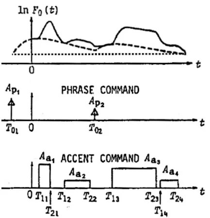
Fb: This is a constant that represents the baseline of the fundamental
frequency. In the present study, it can be thought of as the lowest frequency a specific speaker produces in his or her utterance. The natural logarithm of Fb (ln Fb) is plotted in Figure 1 with a dotted line.
Gp(t): This function models a phrase command (PC). It describes the changes of f0 in part of an utterance that generally corresponds to an intonation phrase (IP). The contours of two successive phrase commands are plotted in Figure 1 with a dashed line.
Each phrase command has a constant parameter T0i4 that denotes
its timing. To model different amplitudes in f0, each instance of
Gp(t) has a magnitude parameter Api5. The sum of all phrase
4
The subscript i denotes the index of the phrase command inside the utterance.
5 In Figure 1, the A
commands describes the global changes of f0 in an utterance. It is
called the phrase component of f0. According to Leemann (2012:
50), the phrase component is "suitable to describe the general declination tendency in intonation contours since the contour of a phrase component rises quickly and decreases gradually towards the asymptotic value Fb".
Ga(t): This function models an accent command (AC).They are added on top of the phrase commands. Accent commands represent fast, local changes of f0. According to Leemann (2012: 54), they are
generally responsible for local prominence marking on syllables.
The contours of four accent commands are plotted in Figure 1 with a solid line.
Each accent command has the constant timing parameters T1j6
(start of AC) and T2j (end of AC). The heights of the accent
commands are expressed by the amplitude parameter Aaj. The
sum of all accent commands describes the local changes of f0 in
an utterance. It is called the accent component of f0.
In the terminology of the Fujisaki model, Gp(t) and Ga(t) are called control mechanisms. Figure 1 illustrates their influence on the contour of ln F0(t).
Fig. 1: The Fujisaki intonation model including phrase and accent commands (adopted from Fujisaki (1984: 235), modified by Peter). AC amplitude corresponds to the height of the rectangles in the "Accent Command" subplot.
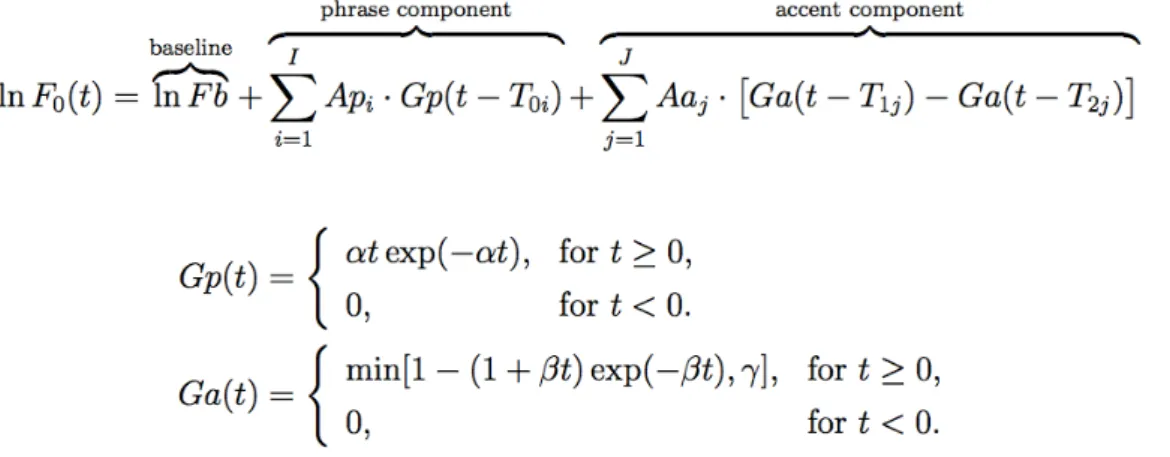
Using the above functions, any recorded utterance can be modeled mathematically. Figure 2 contains the complete formula underlying the Fujisaki model (Leemann, 2012: 43).
Fig. 2: The interpolation formula of the Fujisaki model. The constants α, β, and ɣ were set to 2.0/sec, 20.0/sec, and 0.9/sec respectively. For more information on the mathematical formulation, see Leemann (2012: 143-144).
In practice, the presence and shape of phrase and accent commands are determined manually by means of an f0-curve-fitting editor developed by Fujisaki (Fujiparaeditor).
1.2
Statistical analysis on AC amplitude by Leemann (2012)
Leemann’s (2012) analysis of spontaneous speech intonation contours in four Swiss German dialects aimed at the creation of dialect-specific multiple linear regression models. These models, generated for the most relevant of Fujisaki model parameters, allowed for a distillation of the relative contribution of independent variables (incorporating linguistic
variables such as stress and word class; paralinguistic variables like
phrase type and focus; as well as non-linguistic variables such as sex) towards explaining f0 variation in each of the model parameters.
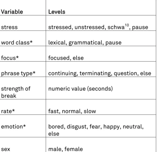
To make sure that the results of the statistical analyses allow for an immediate linguistic interpretation, Leemann (2012) considers only the explanatory variables stress (i.e. lexical stress), word class, focus7, phrase type, strength of break8, rate9, emotion, and sex for his statistical analysis of the AC amplitude behavior. Table 1 gives an overview of all the levels.
7 The variable
focus stands for a deliberate emphasis made by the speaker. See Leemann (2012: 127ff.) for further explanations.
8
The variable strength of break corresponds to the length of the pause between the current and the previous intonation phrase and is measured in seconds.
9 Based on the number of syllables produced per second, each speaker was attributed one of
Variable Levels
stress stressed, unstressed, schwa10, pause
word class* lexical, grammatical, pause
focus* focused, else
phrase type* continuing, terminating, question, else
strength of break
numeric value (seconds)
rate* fast, normal, slow
emotion* bored, disgust, fear, happy, neutral,
else
sex male, female
Table 1: Explanatory variables in Leemann (2012). Significant predictors for AC amplitude are marked with an asterisk (*).
After an initial effect screening, the subset of significant explanatory variables is deduced using multiple linear regressions. As for the AC
amplitude of the Valais dialect, the variables phrase type, rate, focus,
emotion, and word class turn out to be significant. The fact that the
variable stress is not a relevant predictor ties in nicely with the existing
research literature mentioned in section 1, i.e. stress as an independent
variable seems to have little effect on local f0 contours in the Valais dialect.
The adjusted coefficient of determination11 of 9% suggests, however, that
most of the variability in the AC amplitude cannot be explained by these variables (Leemann, 2012: 282 ff.).
What does it mean if one was to predict the placement and the amplitude of local accents based on these variables? Will 91% of our predictions be wrong? With respect to the placement, the amplitude, or even both? Is Wipf possibly right, after all, in stating that "people place accents as strongly as
10
In Peter (2011), the schwa level was merged with the unstressed level. The existence of a schwa in the nucleus is captured by a separate variable (nucleusSchwa).
11 The coefficient of determination (R2) is a statistical measure that provides information
about the goodness of fit. It is bounded by 0 and 1 and is a measure for the overall variability that can be accounted for by the variables in the model.
possible on the most irrelevant of syllables" (1910: 19)? Or could scientific computing methods yield some new insights?
1.3
Motivation behind the new approach
The analysis conducted by Peter (2011) is geared towards answering the following two questions:
1. Is it possible to predict the local voice fundamental frequency changes in the Valais dialect by means of scientific computing techniques?
2. If so, to what extent can we gain linguistic insights from these results?
The first question is mainly motivated by the fact that scientific computation is already being applied in a plethora of scientific fields as diverse as electronics, economics, or meteorology. In each of these fields, it is used to solve complex problems that typically lack a straightforward analytic solution. The method chosen by Peter (2011) is called Linear Least
Squares by SVD12 (see subsection 2.1). It is adopted from Gonnet and Scholl
(2009: 33–48) who show how it can be used in molecular biology to predict the secondary structure of proteins. The central point of interest is how well this algorithm will perform on the prediction of the local intonation contours of Valais Swiss German, which seems to be a notoriously thorny problem.
But even if the above approach should work to make reliable predictions, it is not guaranteed that one also obtains linguistic insights. Scientific computation is primarily about solving mathematical models, so finding an enlightening explanation for the optimal solution in the framework of the problem domain can still be difficult. This aspect is covered by means of the second question.
2. Analysis
In this section we will first give a short description of Linear Least Squares by SVD. Next, we will present its application to Valais Swiss German speech data (Peter, 2011: 16–21). The last subsection is devoted to Peter’s validation criteria of the analysis results (2011: 14–16)13.
12 SVD stands for Singular Value Decomposition.
13 In the validation component, we evaluate the fit of the model with respect to factors that are
2.1
Linear Least Squares by SVD
In order to apply Linear Least Squares (henceforth referred to as LLS) by SVD to a problem, the mathematical model needs to have the shape of a set of linear equations with numeric variables. A single equation (corresponding to a single row in our dataset) would basically have the following form:
acAmplitude = a0 + a1 · wordClass + a2 · emotionNeutral + a3 · emotionBored + …
The left hand side of the equations contains the response variable. In our
case this is the variable for the AC amplitude acAmplitude14. The right hand
side of each equation consists of the sum of the explanatory variables that
are scaled by linear parameters a015, a1, …, an. These parameters are the
unknowns of the model. Intuitively, the larger a parameter, the greater is the impact of the corresponding variable value onto the response variable on the left hand side.
In order to integrate categorical variables like emotion in the model, we convert each of their variants into a separate variable that can only assume
the value 1 (standing for present) or 0 (standing for absent)16. So a token
with the emotion variant neutral is represented by the emotionNeutral variable set to 1 and all the other emotion variables (like emotionBored, emotionDisgust, etc.) set to 0.
This approach of variable splitting may look tedious, but it actually brings about a significant analytical advantage. Since each of the variants is accompanied by a separate parameter, it is possible to see the individual effects on the AC amplitude directly. Variables that have a parameter with a positive sign are AC amplitude boosters whereas variables with negative parameters are AC amplitude suppressors.
The output of the LLS by SVD algorithm are the optimal parameters a0, a1, …,
an17. Based on these values, the relative importance of each explanatory
variable can be deduced by calculating its contribution to the reduction of the residual norm, which is a measure for evaluating the fit of the model with respect to the data (Peter, 2011: 18).
14 The absence of an AC was treated as an AC amplitude of 0. 15 a
0 is not attached to a variable. It is for coping with a constant bias between the values on
both sides of the equation.
16
In programming, these sort of variables are typically called Boolean.
17 High efficiency and robustness against linear dependencies are two of the most important
2.2
Application to Valais Swiss German
The analysis by Peter (2011) is based on speech data that was collected by Leemann in a secondary school in the city of Brig, Canton of Valais. It comprises 578 annotated utterances that were elicited in the course of narrative interviews with ten different students (Leemann, 2012). Both sexes are represented equally. The total length of the audio material is approximately 45 minutes.
Each utterance had been transcribed and annotated on the syllable level in
Praat. This metadata was later transferred to a spreadsheet file. LLS by SVD was applied to a filtered and transcoded version of this file.
The first model by Peter (2011) basically comprises the same variables as Leemann (2012) used for his analysis of the AC amplitude. But, as
mentioned above, the variants of the categorical variables emotion and
phraseType were transformed into distinct Boolean 18 variables (like
emotionHappy, emotionBored, etc.)19. In Leemann (2012), nucleusSchwa
(representing the presence of a schwa sound in the syllable nucleus) was treated as a value of the variable stress (see Table 1). In Peter (2011), it was
handled as a separate Boolean variable. The Boolean variable segment was
added to distinguish between real speech segments and pauses. In
Leemann (2012), this distinction was only made in the variables stress and
wordClass. Furthermore, the variable rate was assigned the numeric values for the syllables produced per second instead of the categorical variants
fast, normal, slow used by Leemann (2012). Finally, the variable wordClass
was made Boolean as well by assigning level 1 to all lexical segments and 0 to other segments.
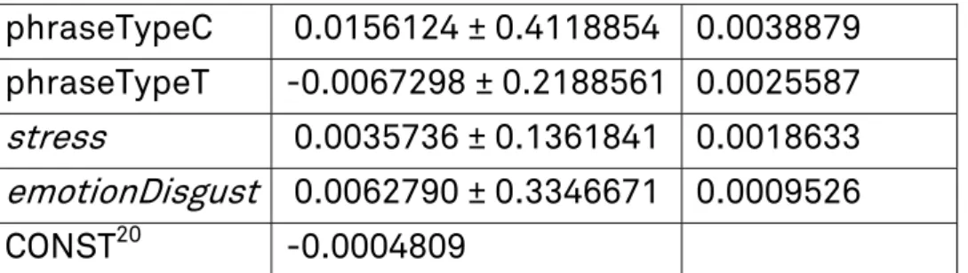
Variable Parameter σ Norm Decrease
focus 0.0601437 ± 0.1566642 0.3988164 wordClass 0.0373295 ± 0.1329001 0.2134935 segment 0.0428703 ± 0.2164096 0.1061920 nucleusSchwa 0.0145203 ± 0.1450973 0.0270996 emotionHappy 0.0197854 ± 0.2611131 0.0155369 emotionBored -0.0200338 ± 0.2884133 0.0130566 rate 0.0007263 ± 0.0159460 0.0056139 emotionNeutral 0.0069269 ± 0.1674181 0.0046324 18
A Boolean variable has only two levels. Generally, level 1 stands for yes (or present) while level 0 means no (or absent).
19
phraseTypeC 0.0156124 ± 0.4118854 0.0038879 phraseTypeT -0.0067298 ± 0.2188561 0.0025587
stress 0.0035736 ± 0.1361841 0.0018633
emotionDisgust 0.0062790 ± 0.3346671 0.0009526
CONST20 -0.0004809
Table 2: LLS parameter, standard deviations, and norm decrease of the variables in the initial model. Adopted from Peter (2011: 19).
As can be seen in Table 2, the variable focus turned out to be by far most
influential when it comes to raising AC amplitudes. This is intuitively plausible since local f0 changes are primarily responsible for prominence marking (Leemann, 2012: 65). A look into the complete dataset confirms this finding: As a matter of fact, 86% of the focused speech segments also have an AC.
The second most important variable is wordClass. Although it is considered
significant in Leemann’s analysis as well, it is held responsible for a relative contribution of only 3% (2012: 255) Again, a preliminary analysis of the data shows that 82% of the lexical segments have an AC while 18% do not. As for the non-lexical segments, however, only 67% are part of an AC while 33%
are not accented21. There is also a noteworthy difference with respect to
the average AC amplitude: For lexical segments it is 0.208 ln Hz whereas for grammatical segments it is 0.190 ln Hz.
Not surprisingly, the third most important variable is segment. As
mentioned, this variable was included to distinguish between real speech segments and pauses. Its positive parameter value proves that real segments have a much bigger chance of carrying ACs than pauses, which is not much of an astonishing insight. All in all, the above three variables have the greatest positive influence on the AC amplitude.
A bit bewildering, however, is the relatively high ranking of nucleusSchwa
since, intuitively, we associate schwa with unstressed syllables. But, as mentioned above, the analysis of Leemann’s data proves that an astonishing share of 76% of schwa syllables in fact are spanned by an AC.
The two emotion variables emotionHappy and emotionBored also have an
influence on AC amplitudes, the former in a positive (i.e. amplitude increasing manner), the latter in a negative (i.e. amplitude decreasing, see negative sign of parameter) way. Again, this sounds logical since the f0 of a
20 CONST is a variable whose only purpose is to even out a constant bias in the equations. Its
parameter corresponds to a0 in section 2.1.
21 As a matter of fact, a share of AC-carrying non-lexical segments of 67% looks unusually high.
We see it as a manifestation of the free pitch accent in Valais Swiss German (Wipf, 1910: 19) which gives it a singing quality (Stalder, 1819: 7-8).
happy (or excited) person generally sounds more variable while the f0 of a bored person tends to be monotonous.
The contribution of the remaining factors to the norm decrease is less than 2% of the largest norm decrease (by the factor focus), so they have virtually no influence on local accents. As already noted by scholars like Wipf (1910) and Leemann (2012), this also includes lexical stress.
2.3
Validation
About 50% of Leemann’s speech data had been spared for the validation of
the obtained parameters22. The validation process applies the parameters
obtained in the previous step to the explanatory variables of the validation dataset and compares the result, i.e. the predicted AC amplitude (acAmplitude′), with the actually measured AC amplitude (acAmplitude). The deviation is measured in terms of the absolute difference.
acAmplitude’ a0 + a1 · wordClass + a2 · emotionNeutral + a3 · emotionBored + … deviation |acAmplitude − acAmplitude′|
In Peter (2011), the quality of the predictions were validated with respect to the following three criteria:
1. AC placement: The model should be able to distinguish between speech segments that carry an AC and speech segments that do not. 2. Average AC amplitude deviation: The model should be able to predict
the amplitude of the ACs as accurately as possible.
3. AC boundaries: The model should be able to predict the boundaries between successive ACs correctly.
The first criterion AC placement can be validated quite easily since the
prediction for a given speech segment can only be either true or false23. But
since we are dealing with a simplified model of reality, the predicted AC amplitudes of syllables that do not carry an AC will never be exactly 0 (as in the dataset) but some small value around 0. So we need a mechanism to tell "real" amplitudes (belonging to speech segments that do carry an AC) from "false" amplitudes (belonging to speech segments that do not carry an
AC). This is achieved by setting a border value d0 that yields the best
separation with respect to the training data. Every amplitude that is larger
than d0 is considered real whereas speech segments with AC amplitudes
smaller than d0 are considered to be lacking an AC. In the model presented
above, the optimal d0 value turned out to be 0.0464 ln Hz.
22 In Peter (2011), the utterances of each speaker were divided equally between the training
and the validation set.
23 Wrong predictions can either be false positives, i.e. predicting an AC where there is actually
The output of the validation is the percentage of speech segments that were classified correctly. A hit rate of 50% would be equal to random
guessing24, so, in any case, an acceptable model has to provide a rate that
is significantly higher.
The second criterion "average AC amplitude deviation" is a continuous value. It should be clearly smaller than the average AC amplitude, and, ideally, less than the smallest AC amplitude.
The third criterion "AC boundaries" is motivated by the following two observations:
1. ACs more often than not span several speech segments.
2. ACs often occur directly one after another (i.e. without a gap in between).
In order to predict local f0 behavior accurately, it is crucial to decide which segments that carry an AC amplitude belong to the same AC. This is not an easy undertaking because, as with the "false" amplitudes mentioned above, adjacent speech segments belonging to the same AC will never have exactly the same AC amplitude in the prediction (unless they are absolutely identical with respect to the explanatory variables). This means that we
have to find once again a border value b0 that distinguishes between "AC
continuations" and "AC boundaries". In other words, when the AC amplitude difference between two successive speech segments is less
than b0, they belong to the same AC. When it is greater than b0, we assume
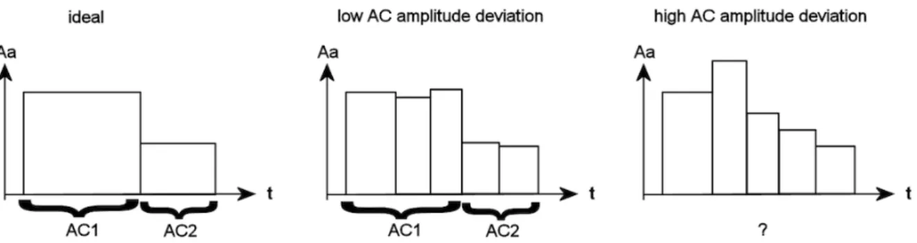
that they belong to different ACs. In this respect, the second criterion has an important influence on the third: The higher the average AC amplitude deviation, the more difficult it gets to locate boundaries between adjacent
ACs (see figure 3). In the model presented above, the optimal b0 value
turned out to be 0.1549 ln Hz.
24 Imagine a dependent variable that has two variants, one of which is much rarer than the
other one (say 5% vs. 95%). Then a program that always predicts the frequent variant and never the rare one would have 95% accuracy. But this is clearly not what we want. In Leemann’s dataset, 66.4% of the speech segments carry an AC whereas only 33.6% do not. Since both the presence and the absence of ACs are supposed to be predictable with equal reliability, the LLS algorithm was weighted to prevent a bias in favor of AC-carrying segments. See Gonnet and Scholl (2009) for more details.
The validation of the above model produced the following results.
AC placement: 77% (or 4220 out of 5446) of the speech segments were classified correctly.
Average AC amplitude deviation: 0.1132 ln Hz (smallest/average/largest AC amplitude: 0.0408 / 0.2033 / 0.8163 ln Hz)
AC boundaries: 590 classification errors (number of AC boundaries: 590) The fact that the AC placement detection rate is clearly above 50% proves that the model has indeed captured important characteristics. The average AC amplitude deviation (0.1132 ln Hz) is about half the size of the average AC amplitude. This is obviously far too large for detecting boundaries between adjacent ACs: As the data suggests, probably all AC boundaries went undetected. In other words, successive ACs are always merged to one large AC. If we applied this behavior to the audio recording of an utterance, contours with variable f0 activity would be leveled out, which would result
in flat, monotonous intonation.25
By introducing additional variables (such as sex, duration, nucleus type,
syllable position, etc.) AC placement can be increased to 80% and the average AC amplitude deviation can be decreased to 0.1075745, yet this has no significant effect on the detection of AC boundaries, which still fails to work (Peter, 2011: 21–24).
3. Discussion
We believe that the above inaccuracies can be attributed to two different causes. The first one concerns the limited amount of annotated speech data. Peter’s analysis is based on 45 minutes of audio material, half of which is used as test data. This means that the model is essentially trained
25 Actually, the flat contours are also a consequence of our AC synthesis approach. After
identifying a multi-syllable AC, we took the average of the predicted AC amplitudes of the syllables. So when we mistook two successive ACs as one AC, the resulting accent is longer and more levelled out.
on only 22.5 minutes of speech. So additional speech data is very likely to improve the validation results.
The second reason may be the lack of paralinguistic factors included in the
analyses by Leemann (2012). Zemp (2008), who studied the intonation contours of calling names in Lucerne Swiss German, identified distinct intonation patterns for a few paralinguistic types, such as "wheedling", "warning", and "reproachful". He pointed out the significance of including paralinguistic information for f0 modeling in dialectal speech data. Before we could add this kind of paralinguistic factors to our intonation model of Valais Swiss German, however, we would of course first have to qualitatively assess the corpus for a refined analysis and identification of paralinguistic factors. And even if we had perfect descriptions of all existing paralinguistic patterns, they may take an odd shape when
translated into accent command patterns26. After all, the concept of an
accent command is only useful for locally restricted rise-fall pairs with a
more or less symmetrical shape27. This may usually be the case for local
contours that are caused by lexical stress. But studies on paralinguistic f0
features have shown that even single movements (such as a steep fall)
carry paralinguistic meaning and that sequences of movements (such as "rise steep fall rise" for a "warning wheedling" meaning) can span over different numbers of syllables (see for example Zemp, 2008). Obviously, this cannot be captured well in a syllable-based model working with local accents. So one of the future challenges will be to work out a
double-layered model that is able to accommodate both linguistic and
paralinguistic f0 movements. The submodel for linguistic movements could be built on syllable-based data segmentation and some concept of "local accent" whereas the paralinguistic submodel would rather have a metrical data segmentation and conceptualize in terms of single f0 movements.
4. Conclusions
The goal of Peter (2011) was to find out (1) whether scientific computing techniques could shed light on the f0 contours in the VS dialect and (2) to what extent linguistic insights could be gained from the results. Although the presented model is far from perfect, the good results that could be achieved with respect to the detection of local accent contours justify
26 Zemp (2008) describes intonation patterns in the framework of autosegmental-metrical
phonology (Pierrehumbert, 1980 and Silverman et al., 1992) and additional annotation tiers where relative intervals are captured (measured in semitones). This way of analyzing pitch is in line with the concept of “timbre-based melody” put forth by Minematsu und Nishimura (2008). According to the latter, human beings are usually unaware of absolute pitch in sounds. What is actually perceived are the pitch movements over time (“relative pitch”).
27 Basically, the Fujisaki model allows superposition of accent commands to interpolate any
sort of intonation contour. Whether this is an intuitive model of the underlying mechanisms is a different question.
answering (1) with a "YES". In our opinion, the inability of the present model to separate successive local accents can be attributed to the limited amount of training data and missing paralinguistic factors (whose investigation is beyond the scope of the present study). As for (2), the results clearly confirmed several qualitative observations with respect to f0 peculiarities in the Valais dialect, such as the independence of pitch accent placement from lexical stress. So the application of Linear Least Squares by SVD can indeed yield linguistically valuable insights.
Bibliography
Fujisaki, H. (1984): Analysis of voice fundamental frequency contours for declarative sentences of Japanese. Journal of the Acoustical Society of Japan, 5 (4), 233-42.
Gonnet, G. H. & Scholl, R. (2009): Scientific Computation. Cambridge (Cambridge University Press). Leemann, A. (2012): Swiss German Intonation Patters. Amsterdam / Philadelphia (Benjamins). Minematsu, N. & Nishimura, T. (2008): Consideration of infants’ vocal imitation through modeling
speech as timbre-based melody. New Frontiers in Artificial Intelligence, LNAI4914, 26-39. Peter, N. (2011): The local contours of the voice fundamental frequency in the Swiss German
dialect of Valais. Bachelor’s thesis, University of Bern.
Pierrehumbert, J. 1980. The Phonology and Phonetics of English Intonation. Ph.D. Thesis, MIT. Ris, R. (1992): Innerethik der deutschen Schweiz. In: Hugger, P. (Hg.). Handbuch der
schweizerischen Volkskultur, Bd. II. Offizin, 749-766.
Silverman, K. E. A. et al. (1992): TOBI: A Standard for Labelling English Prosody: Proceedings of the 1992 International Conference on Spoken Language Processing, 2, 867-870.
Stalder, F. J. (1819): Die Landessprachen der Schweiz oder Schweizerische Dialektologie. Aarau (Sauerländer).
Werlen, I. & Matter, M. (2004): Z Bäärn bin i gääre: Walliser in Bern. In: Glaser, Elvira et al. (Hg.). Alemannisch im Sprachvergleich: Beiträge zur 14. Arbeitstagung für alemannische Dialektologie in Männedorf (Zürich) vom 16. 18.9.2002. Wiesbaden (Franz Steiner), 263-280. Wipf, E. (1910): Die Mundart von Visperterminen im Wallis. Frauenfeld (Huber).
Zemp, M. (2008): Anredekonturen im Luzerndeutschen: Eine intonationale Teilgrammatik. Arbeitspapiere, Institut für Sprachwissenschaften, Universität Bern, Bd. 44, 1-61.