Correlated exciton dynamics in semiconductor nanostructures

(1)

Correlated exciton dynamics in semiconductor

nanostructures

by

Patrick Wen

B.S. Chemistry, University of California Berkeley (2007)

Submitted to the Department of Chemistry

in partial fulfillment of the requirements for the degree of

Doctor of Philosophy in Chemistry

at the

MASSACHUSETTS INSTITUTE OF TECHNOLOGY

June 2013

ARCHMVS

MASSACHUSETS INSfffE OF TECJHNOLOGY

UL 0 1 2013

BRAR IES

@

Massachusetts Institute of Technology 2013. All rights reserved.

Author...

...

y...

Department

of Chemistry

May 10, 2013

Certified by...

.

.r...

Keith A. Nelson

Professor

Thesis Supervisor

z-)

Accepted by ...

.

...

Robert W. Field

Chair, Department Committee on Graduate Theses

(2)

(3)

This doctoral thesis has been examined by a Committee of the

Department of Chemistry as follows:

Professor Robert G. Griffin...

Chairman, Thesis dPommittee

Professor of Chemistry

Professor Keith A. Nelson...

...

:.

...

. . . ..

Thesis Supervisor

Professor of Chemistry

Professor Robert W . Field ...

Member, Thesis Committee

Haslam and Dewey Professor of Chemistry

(4)

(5)

Correlated exciton dynamics in semiconductor

nanostructures

by

Patrick Wen

Submitted to the Department of Chemistry on May 10, 2013, in partial fulfillment of the

requirements for the degree of Doctor of Philosophy in Chemistry

Abstract

The absorption and dissipation of energy in semiconductor nanostructures are of-ten determined by excited electron dynamics. In semiconductors, one fundamentally important electronic state is an exciton, an excited electron bound to a positively charged vacancy. Excitons can become correlated with other excitons, mutually in-fluencing one another and exhibiting collective properties. The focus of this disserta-tion concerns the origins, effects, and control of correlated excitons in semiconductor nanostructures.

Correlated Coulomb interactions can occur between excitons, resulting in energy shifts and dephasing in each exciton. Two-dimensional Fourier-transform optical spectroscopy is a powerful tool to understand Coulomb correlations; the technique relates exciton dynamics during distinct time periods. However, the technique is still limited by weak spectral features. Using two-dimensional pulse shaping methods, waveforms of excitation fields were tailored to selectively amplify spectral features of correlated exciton states in gallium arsenide quantum wells. With the aid of theo-retical models, 2D spectra of quantum wells revealed clear contributions of Coulomb correlations to the exciton dynamics. Time and power dependent properties of the

2D spectra indicate several mechanisms for exciton interactions that are neglected in

commonly used theoretical models.

If a semiconductor material is fabricated within a microcavity, optical fields can be trapped around the semiconductor, strongly distorting properties of the semiconduc-tor excitons and forming new quasi-particles called exciton-polaritons. Theoretical work has suggested exciton-polariton Coulomb correlation strengths can be reduced compared to that of excitons. Using two-dimensional Fourier-transform optical spec-troscopy, control of Coulomb correlations was demonstrated by varying the cavity structure. The cavity fields were also shown to induce high-order correlated interac-tions among exciton-polaritons.

A macroscopic quantum degenerate system of exciton-polaritons can also become

correlated, exhibiting long-range order typical of a Bose-Einstein condensate. How-ever, unlike a Bose-Einstein condensate, exciton-polartions are not typically in

(6)

ther-mal equilibrium. Using a sample with exciton-polariton lifetimes longer than previous samples, the macroscopic behavior of exciton-polaritons was investigated by imaging the exciton-polariton photoluminescence. Condensation depended significantly on spatially-varying potential energy surfaces. Using optically-induced harmonic po-tential barriers, thermal equilibrium among exciton-polaritons was achieved, with exciton-polaritons forming a Bose-Einstein distribution at densities above and below the condensation phase transition.

Thesis Supervisor: Keith A. Nelson Title: Professor of Chemistry

(7)

Acknowledgments

Many people provided invaluable support throughout my time at MIT: mentors, colleagues, friends, and family. Without these people, the work presented here would not be possible.

My advisor Keith Nelson provided much more than scientific guidance; he was a

constant source of enthusiasm and inspiration. I am very grateful that he has always supported my ideas and work.

Additional guidance came from other mentors in the group. Specifically, Kathy Stone, Duffy Turner, and Kenan Gundogdu taught me how to work in lab and their research inspired many of the ideas in this thesis.

Dylan Arias joined the 2D spectroscopy project at the same time as myself. From learning how to align optics to writing this thesis, his friendship enlivened even the most challenging moments in graduate school. Of course, the times we found reasons to celebrate were even better.

Yongbao Sun toiled in lab with me for the last two years. Chapter 8, in particular, would not be possible without his help. I am very grateful for his hard work, his questions, which pushed me to learn more, his ideas, and his company during those long days and nights in lab.

Several collaborators contributed directly to the research in this thesis with their expertise and advice. Professor Jeremy Baumberg and Gabriel Christmann at the University of Cambridge provided invaluable expertise in the initial exciton-polariton experiments described in Chapter 7. Professor David Snoke at the University of Pittsburgh acted almost as a second advisor for the research described in Chapter 8. Professor Snoke and his students, Bryan Nelsen and Gangqiang Liu, were extremely helpful during those experiments.

The entire Nelson group provided a collegial and fun environment to work in. Challenging experiments and late hours were made so much easier by smart colleagues and good friends.

(8)

who made the transition to MIT so much easier; Kara and Lemon, friends from year one; the Puerto Rico crew; Kevin, Scott, Nicole, and David; everyone who was always ready for the Muddy, a camping trip, or a spontaneous trip to karaoke; and the great

scientists and friends that live in the basement of MIT.

I also need to thank my family: Mom, Dad, and my brother, Aki. Their support and encouragement have been essential during my time at MIT. I have had many fortunate opportunities in my life, which would not be possible without the sacrifices of my parents.

Finally, I need to thank Sharmini, who was there to celebrate my successes, listen to my frustrations, and provide encouragement when I needed it most. Although we have lived in different cities for the last six years, she has shaped my experiences at MIT more than anyone else. I am grateful for her love and support.

(9)

7 Many body interactions of exciton-polaritons in semiconductor mi-crocavities probed by two-dimensional spectroscopy 147 7.1 Evidence of correlated interactions between microcavity polaritons 149 7.2 Correlated interactions controlled by exciton-photon coupling . . . . . 152

7.2.1 Two-polariton interactions probed by two-dimensional spec-troscopy . . . . 152

7.2.2 Theoretical model of correlated two-polariton interactions . . 154

7.2.3 Biexciton strong coupling . . . . 158

7.3 High-order correlations between exciton-polaritons . . . . 159

7.3.1 Three-polariton and four-polariton interactions probed by two-dimensional spectroscopy . . . . 159

7.3.2 Theoretical model of high-order correlations . . . . 162

7.4 Conclusions . . . . 166

8 Polariton condensation 169 8.1 Polariton Bose-Einstein condensation . . . . 171

8.1.1 Theory of Bose-Einstein condensation . . . . 171

8.1.2 Polariton condensation and polariton lasing . . . . 177

8.1.3 Polariton trapping . . . . 180

8.2 M ethods . . . . 182

8.2.1 Characterization of long-lifetime sample . . . . 182

8.2.2 Optical trapping of polaritons . . . . 186

(12)

8.3.1 Thermal properties of long-lifetime polaritons at low excitation

densities . . . . 190

8.3.2 Condensation of untrapped polaritons . . . . 195

8.3.3 Condensation of trapped polaritons . . . . 197

(13)

List of Figures

2-1 2-2 2-3 2-4 2-5 2-6 2-7 2-8 2-9 2-10 2-11 2-12

Third-order Feynman diagrams . . . . Fifth-order Feynman pathway diagrams . . . . Seventh-order Feynman pathway diagrams . . . . Complex 2D correlation spectrum . . . . Cross peaks in 2D spectra . . . . Inhomogeneous broadening in 2D spectra . . . . Two-quantum coherence in 2D spectrum . . . .

2D Fourier transform optical setup based on pulse shaping

Beam shaper . . . . 2D pulse shaper . . . .

Setup to route the local oscillator around sample . . . . Spectral interferometry . . . .

3-1 Feynman diagrams of gallium arsenide quantum well . . . .

3-2 Coherent control pulse parameters . . . .

3-3 2D rephasing and two-quantum spectra of gallium arsenide quantum

w ells . . . . 3-4 Selective enhancements in 2D spectra using a double pulse . . . .

3-5 Selective enhancement in 2D two-quantum spectra using a phase win-dow pulse shape . . . .

3-6 Phase shift caused by phase window pulse shape . . . .

3-7 Calculated 2D two-quantum spectra incorporating phase window pulse

shape... ... . . . . 31 . . . . 34 . . . . 35 . . . . 38 . . . . 39 . . . . 40 . . . . 41 . . . . 46 . . . . 48 . . . . 51 . . . . 52 . . . . 55 60 62 67 69 72 73 74

(14)

4-1 Two-exciton interaction matrix . . . . 89

4-2 Calculated rephasing two-dimensional spectra using the dynamics-controlled truncation schem e . . . . 91

4-3 Calculated two-quantum two-dimensional spectra using the dynamics-controlled truncation scheme . . . . 92

4-4 Hierarchy of differential equations in the modified optical Bloch equations 95 4-5 Calculated rephasing two-dimensional spectra using the modified

op-tical Bloch equations . . . . 100

4-6 Calculated two-quantum two-dimensional spectra using the modified optical Bloch equations . . . . 100 5-1 Electronic energy levels of gallium arsenide quantum wells . . . 107

5-2 Comparison of four-wave mixing signals in two level systems and gal-lium arsenide quantum wells . . . . 108 5-3 Correlation 2D spectra of gallium arsenide quantum wells . . . . 111

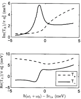
5-4 Correlation 2D spectra of gallium arsenide quantum wells using differ-ent population wait times . . . . 113 5-5 Theoretical real part of two-quantum 2D spectrum of correlated excitons115

5-6 Beam geometry in the Y-shape . . . . 117 5-7 Real part of rephasing two-quantum 2D spectrum of gallium arsenide

quantum wells . . . 118

5-8 Real part of calculated rephasing two-quantum 2D spectrum of gallium

arsenide quantum wells . . . . 120

6-1 _{Structure of a semiconductor microcavity . . . .} ₁₂₅ 6-2 Semiclassical propagation of optical fields in semiconductor microcavity 128

6-3 Calculated optical properties of a semiconductor microcavity . . . . . 130

6-4 Calculated optical properties of polaritons in a semiconductor micro-cavity . . . . 132 6-5 _{Calculated dispersion and detuning properties of polariton modes . .} ₁₃₇ 6-6 Two-dimensional lower polariton dispersion curve . . . . 138

(15)

6-7 Short lifetime semiconductor microcavity sample . . . . 141

6-8 Long lifetime semiconductor microcavity sample . . . . 143

6-9 Optical setup to spectrally resolve and image photoluminescence . . . 144

7-1 Three-quantum fifth-order spectroscopy of polaritons . . . . 148

7-2 spectrally resolved four-wave mixing polariton signals . . . . 150

7-3 Parametric amplification of microcavity polaritons . . . . 151

7-4 Experimental two-quantum 2D spectra of microcavity polaritons . . . 153

7-5 Detuning dependence of R . . . . 155

7-6 Calculated two-quantum 2D spectra of microcavity polaritons . . . . 157

7-7 Three-quantum 2D spectra of microcavity polaritons . . . . 161

7-8 Four-quantum 2D spectra of microcavity polaritons . . . . 162

7-9 Field-coupled correlations in semiconductor microcavities . . . . 162

8-1 Density of states for a uniform 3D, 2D, and ID system . . . . 174

8-2 Distribution of bosons for a uniform 3D system . . . . 174

8-3 Influence of interactions on Bose-Einstein condensates . . . . 176

8-4 Mechanisms of BEC in exciton-polariton systems . . . . 179

8-5 Imaging setup to measure polariton photoluminescence . . . . 183

8-6 Spectrally resolved far-field exciton-polariton photoluminescence in long-lifetim e sam ples . . . . 184

8-7 Spatially filtered spectrally resolved far-field exciton-polariton photo-luminescence in long-lifetime samples . . . . 185

8-8 Exciton-polariton detuning curves in long-lifetime sample . . . . 186

8-9 Propagation of polaritons in long-lifetime samples . . . . 187

8-10 Multiple-spot pumping and imaging setup to optically trap polaritons and measure photoluminescence . . . . 188

8-11 Spectrally resolved near-field images of the optically-induced polariton trap ... .. ... 189

(16)

8-13 Temperature fitting of trapped polaritons for different cavity detuning

energies . . . . 194 8-14 Condensation of untrapped polaritons . . . . 196 8-15 Spectrally resolved near-field image of trapped polariton

photolumi-nescence . . . . 197 8-16 Spectrally resolved far-field images of trapped polariton

photolumines-cence at zero cavity detuning energy . . . . 198 8-17 Temperature fitting of trapped polaritons at zero detuning . . . . 200

8-18 Spectrally resolved far-field images of trapped polariton

photolumines-cence at a cavity detuning energy of 6.8 meV . . . . 201

8-19 Temperature fitting of trapped polaritons at a cavity detuning energy

of 6.8 m eV . . . . 202

8-20 Spectrally resolved far-field image of trapped polariton

photolumines-cence at a cavity detuning energy of -5 meV . . . . 203 8-21 Temperature fitting of trapped polaritons at a cavity detuning energy

of -5 m eV . . . . 204 8-22 Temperature fitting of trapped polaritons at a cavity detuning energy

of -5 meV above condensation threshold . . . . 204

8-23 Distribution of polaritons at different temperatures . . . . 207

(17)

Chapter 1 Introduction

1.1 Motivation and background

Nanomaterials have been used by humans for centuries. By dispersing gold or sil-ver nanoparticles into molten glass, ancient glassmakers created stained glass that reflected red or yellow light[99]. In the last several decades, with the advent of techniques such as scanning tunneling microscopy[42], scientists and engineers have achieved much of the dream that Richard Feynman laid out in his seminal lecture "Plenty of Room at the Bottom"[45]: the properties of materials can be engineered atom by atom. Nanomaterials fabricated from semiconductor materials have at-tracted perhaps the most attention, especially towards goals of solving global energy challenges[59] and engineering technologies for next-generation computers[74].

Of fundamental importance to semiconductor nanomaterials is the exciton[46, 153], an electron that is excited into a high energy state but remains bound to the

vacancy left behind in the valence band by the electron. Excitons are often the lowest energy excited state of a semiconductor material and play an important role in the properties of semiconductors; how energy is absorbed and dissipated by a semicon-ductor material is often largely determined by how an exciton absorbs or dissipates energy. In turn, properties of an exciton can be controlled through the engineering of the semiconductor nanostructure. For example, the confinement of exciton wavefunc-tions determines the emission spectrum in quantum dot light-emitting diodes[106, 72].

(18)

Excitons can be correlated with other excitons, mutually influencing each other so that the excitons are best described as a combined system rather than individual excitons. The correlations between excitons can originate from several sources and have profound effects on properties of semiconductor materials. Coulomb interactions between excitons can correlate the time evolution of excitons, modifying the energies and relaxation of the correlated excitons[30]. Excitons can also become correlated through the formation of a macroscopic quantum degenerate system, which is possible due to the bosonic nature of excitons, exhibiting properties typically associated with a Bose-Einstein condensate[19, 68]: long-range order and coherence over the entire system of degenerate excitons. In either case, by exploiting or even controlling how excitons correlate with each other, semiconductor nanomaterials can be engineered to control how energy is absorbed or evolves in the material.

One possible method to control the correlations between excitons is through op-tical fields, which can couple to the charges of excitons, driving the dynamics of the excitons in space and time. Under the right circumstances, excitons can be strongly influenced by optical fields such that the excitons are best described as new particles called exciton-polaritons[53, 54, 47]. One method to create exciton-polaritons is to trap optical fields around semiconductor materials using a microcavity[156], a cavity that is engineered to precisely control how the trapped optical fields interact with the

semiconductor material.

This dissertation is focused on the origins, effects, and control of correlated exci-tons and exciton-polariexci-tons in semiconductor nanostructures. There are three main types of correlations described in this work: Coulomb correlations between excitons, Coulomb correlations between exciton-polaritons, and macroscopic exciton-polariton correlations. In the remainder of this section, a qualitative overview is provided of the correlations and the challenges associated with understanding these correlations.

1.1.1 Correlated Coulomb interactions between excitons

Because an exciton is composed of a pair of positive and negative charges, excitons can interact with other excitons through Coulomb forces. The charges can repel and

(19)

attract one another, causing excitons to scatter with each other. However, the number of excitons and states in a typical semiconductor material cause the Coulomb inter-actions to become quite complex: interinter-actions between two excitons, for example, are influenced by other excitons and carriers, causing the interaction between the two excitons to evolve in a complex manner[30]. This complex interaction between two excitons is called a four-particle correlation (or two-exciton correlation) [11]. Four-particle correlations can have very important effects on exciton nonlinear dynamics; the energies and relaxation times of an exciton can be strongly modified by the cor-related interaction with another exciton. Two excitons of opposite spin, for example, can become correlated so that the two negative charges orbit around the two positive charges, analogous to the formation of a hydrogen molecule, lowering the combined energy of both excitons[83].

In the last decade, the understanding of multi-exciton correlations has been ad-vanced by the development of two-dimensional Fourier-transform optical spectroscopy

(2D FT OPT) [57], which can directly resolve coherences of multiple excitons. Using 2D FT OPT, correlated interactions between two excitons[132, 60], three excitons[140],

and free carriers with excitons[88] have been directly resolved. Despite these advances,

2D FT OPT can still be limited by weak signal or overlapping spectral features, both

of which can obscure the interpretation of spectra. In Chapter 3, methods to se-lectively amplify spectral features in 2D FT OPT are presented. It is shown that

by coherently controlling the excited state dynamics in an exciton system, specific

exciton and multiexciton spectral features can be enhanced in 2D FT OPT. The complexity of correlated Coulomb interactions is another major challenge. Major ap-proximations in the theoretical descriptions of Coulomb correlations limit the sources for correlated interactions to include only coherent excitons[123] and excitons excited in the limit of perturbation theory[11]. Chapter 5 discusses two experiments using

(20)

1.1.2 Correlated interactions between exciton-polaritons

Exciton-polaritons can be formed inside of semiconductor microcavities that trap optical fields around a semiconductor material. Trapped optical fields can generate exciton polarizations in the semiconductor material. In turn, the exciton polarizations can generate optical fields that remain trapped within the cavity and are reabsorbed

by the semiconductor material. The rapid exchange of energy between the cavity

field and the semiconductor material distorts the exciton polarization[65], splitting the resonance energy of the exciton into new energies, and causing the system to be better described as an exciton-polariton[53, 54, 47].

The trapped optical fields can also alter the correlated interactions between exci-tons. By distorting the exciton energies, the correlated motions of multiple excitons can also be modified. Theoretical work suggests that correlations can be significantly reduced by tuning the coupling between excitons and cavity fields which can reduce correlation-induced dephasing [80, 120]. Chapter 7 discusses a set of experiments that directly resolve exciton-polariton correlations using 2D FT-OPT. The exper-iments clearly indicate that a semiconductor microcavity can be used to tune the strength of correlated interactions. The experiments also clearly resolve correlations between three and four polaritons, a higher number of correlated particles than ob-served in semiconductor materials that are not embedded inside of a microcavity. The results indicate a new source for correlated interactions: trapped optical fields can cause polaritons to mutually influence one another.

1.1.3 Spontaneous macroscopic correlations

Under the right conditions, exciton-polaritons can spontaneously form a macroscopic quantum degenerate system in the ground polariton state[37]. The quantum degener-ate polaritons exhibit many of the properties of a Bose-Einstein condensdegener-ate including spontaneous long-range coherence and superfluid propagation[37, 62, 13, 7]. Because of the small effective mass of polaritons, reduced by about eight orders of magnitude compared to the mass of rubidium, room temperature Bose-Einstein condensation

(21)

is theoretically possible[19, 68, 32]. Semiconductor microcavities could also be in-tegrated into solid-state devices; several experiments have demonstrated the use of polariton condensates as ultrafast switches[4] and transistors[14,. 48].

Although quantum degenerate polaritons exhibit many of the properties of a Bose-Einstein condensate, there is significant controversy regarding whether polari-tons truly qualify as a Bose-Einstein condensate[129, 26, 27, 38]. In particular, Bose-Einstein condensation is a phase transition driven by the thermodynamic prop-erties of a system of bosons[43]. Exciton-polaritons, however, are often well in-sulated from phonon interactions, preventing polaritons from establishing thermal equilibrium [135].

Recently, new progress in sample fabrication has improved the lifetime of polari-tons, by at least an order of magnitude, pushing polariton lifetimes into the realm of thermal equilibrium[100]. Chapter 8 discusses the thermodynamic properties of long lifetime polaritons and polariton condensates. The chapter describes how optically-induced harmonic barriers can manipulate the thermodynamic properties of polari-tons, causing polaritons to be in thermal equilibrium throughout a condensation phase transition.

1.2 Outline of dissertation

The dissertation is organized as follows. In Chapter 2, 2D FT OPT is discussed includ-ing the theoretical background and the methods and instruments used. In Chapter 3, techniques are shown to selectively enhance spectral features in 2D spectra. In Chap-ter 4, the origins of many-body inChap-teractions are described using both microscopic and phenomenological theories. In Chapter 5, experiments focused on understanding many-body interactions in gallium arsenide quantum wells using 2D FT OPT are discussed. In Chapter 6, the physical origins of exciton-polariton states in semicon-ductor microcavities are described using both a semiclassical approximation and a full quantum framework. The chapter also describes the semiconductor microcavity sam-ples used in the next two chapters. In Chapter 7, the Coulomb correlations between

(22)

exciton-polaritons, and the strong influence of the cavity field on the correlations, are discussed. In Chapter 8, the Bose-Einstein condensation of exciton-polaritons is discussed. The chapter presents experiments demonstrating how optical trapping of polaritons can control the thermodynamic properties of a polariton condensate.

(23)

Chapter 2 Two-dimensional Fourier transform

optical spectroscopy

Two-dimensional Fourier transform optical spectroscopy (2D FT OPT) is a type of coherent nonlinear spectroscopy that can provide unprecedented insight into the nonlinear electronic response of material. As with other types of coherent nonlinear spectroscopy, 2D FT OPT is based on the excitation of a material using coherent fields of light: microscopic dipoles in the material become excited by coherent fields, evolve in time, and eventually emit a signal field. The energies of the emitted light can be used to understand the excited states of the dipoles. In 2D FT OPT, not only are emission energies recorded, but the emission energies are correlated to an initial excitation energy providing clear experimental signatures of the nonlinear dynamics of the dipoles. 2D FT OPT is a direct extension of 2D FT infrared spectroscopy[102, 69],

which was developed to study the nonlinear vibrational responses of materials. In turn, 2D FT infrared spectroscopy is an analog of 2D NMR spectroscopy[16], which can be used to study the nonlinear nuclear spin responses of materials.

2D FT OPT, and multidimensional spectroscopy in general, provide several

ad-vantages over one-dimensional spectroscopy: congested spectral features are spread over two dimensions, coupled states can be directly resolved as cross-peaks, inhomo-geneous broadening can be separated from homoinhomo-geneous broadening, and multiple-quantum coherences can be directly resolved[57]. Despite the advantages of

(24)

mul-tidimensional spectroscopy, 2D spectra are still plagued by many of the difficulties associated with one-dimensional spectra. In particular, spectral congestion and weak transition dipoles can still make the collection and analysis of 2D spectra difficult. One possible method to overcome these challenges is to use waveforms that can se-lectively enhance the signal for target peaks in 2D spectra, as demonstrated for 2D

NMR[147].

In this chapter, 2D FT OPT is discussed. In the first section, the theoretical back-ground for coherent nonlinear spectroscopy and Fourier-transform multidimensional spectroscopy are described. In the second section, the methods to achieve 2D FT OPT, using 2D pulse shaping, are described. The experimental methods described in this section are also relevant to the results in Chapters 5 and 7. Additional methods to selectively enhance peaks in 2D spectra are demonstrated in the next chapter.

2.1 Theoretical description of two-dimensional Fourier

transform optical spectroscopy

2.1.1 Semiclassical description of coherent nonlinear

spec-troscopy

A theoretical description of coherent nonlinear spectroscopy is derived in this section.

The purpose of the theoretical description is to understand how electric fields can induce a nonlinear response in a material of interest and how the nonlinear response can be detected in spectra. The interaction between electric fields with a material of interest is described semiclassically: electric fields are treated as classical electro-magnetic waves and the material response to the electric fields is derived from the quantum microscopic description of the material. This approach has become widely used to describe nonlinear spectroscopy[97, 57, 31, 138], because the description can provide an intuitive framework for understanding nonlinear spectroscopy and still accurately describe common experimental conditions of nonlinear spectroscopy.

(25)

material. The coherent fields excite dipoles in the material, such as those associated with vibrational modes or electronic excited states. The macroscopic collection of all dipoles excited by the coherent fields results in a polarization:

P(r, t) = pm(t)o(r - rm) (2.1)

where pm(t) is the time-dependent dipole (i.e. charge displacement) at rm that is driven by the electric fields. pm(t) includes all charges that are displaced at rm. The polarizations oscillate, generating additional electric fields as described by the wave equation:

c2 8a2 E(r, t) = 47r 2P(r,t) _(2.2) where c is the speed of light, E(r, t) is an electric field, and P(r, t) is the polarization of the material. Note that although E(r, t) and P(r, t) are vectors, only one polarization component is considered in this chapter to simplify the mathematical description. The electric fields generated by P(r, t) depend on the dipoles excited in the material and are often called signal fields because properties of the fields (e.g. spectral features) can be used to understand properties of the material. In order to solve Equation 2.2,

P(r, t) must be derived.

Derivation of nonlinear polarization

The macroscopic polarization, P(r, t), can be derived from the microscopic response of the material to electric fields. Considering a material that is spatially homogeneous, Equation 2.1 is simplified so that the polarization is given by the dipole expectation value: P(t) =< p(t) >. In order to find < p(t) >, the state of the material needs to be found as a function of time. Using the density matrix formalism in the Schrodinger picture, the state of the material is given by the time-dependent density matrix, p(t), and < p(t) > can be solved by taking the trace of the time-independent dipole matrix,

(26)

p, with p(t):

P(t) =< p(t) > ₍₂₃₎

= Tr[pp(t)]

Of course, in order to solve Equation 2.3, p(t) must also be solved.

p(t) evolves in time because of the influence of a potential created by the electric fields, V(t) = p -E(t). V(t) describes the action of the electric field, E(t), on dipole

transitions in the material. The time dependence of p(t) can be solved using pertur-bation theory: the electric field and density matrix are expanded to different orders in the field amplitude. The total Hamiltonian of the material under the influence of

V(t) is:

-H = n o

+V(t)

(2.4)

where 7Ho is the material Hamiltonian. The time evolution of the density matrix is given by the Liouville-Von Neumann equation:

a_=

-IVI(t)

I,

(t )]

_(2.5)

at

h

where the potential and the density matrix have been transformed into the interaction picture, V1(t) = UV(t)Uo and pI(t) = Utp(t)Uo with Uo = exp(-iHot). Equation 2.5 can be solved by integrating both sides of the equation from an initial time point, to, to a time variable, t:

pI(t) = pi (to) - f dt1[VI(ti, p, (ti)] (2.6)

pI(to) is just the initial value of the density matrix. In a nonlinear spectroscopy

exper-iment, usually pI(to) is given by equilibrium conditions of the material. Equation 2.6 gives the density matrix in terms of the initial density matrix and a density matrix during a new time variable, t1. By iteratively inserting Equation 2.6 into itself, pi(t)

(27)

can be solved exactly using the following equation: p1(t) =p1(to) - iJdt1[V(t1),p(t)]+ +(

J

dt2 dt1 [V1(t2), [V1(t1), pI(to)]] + ... n-1 t2 + ( " dn dtn_1... dt1 [V(tn), [V(tn_1), .. [V(t1), p1(t)] ] ton t to to (2.7)

Equation 2.7 gives the solution to p(t) as a sum of terms, where each term depends on the perturbing electric fields to different orders: the first term on the right hand side of Equation 2.7 does not depend at all on the electric fields, the second term has a first-order dependence on the electric fields, the third term has a second-order dependence, and so on. For fields that are not too strong, p(t) can be accurately solved by truncating Equation 2.7 up to a certain order determined by the strength of the electric fields that interact with the material.

Finally, P(t) can be solved up to a specific order in the electric field by inserting Equation 2.7 into Equation 2.3 and truncating the density matrix terms up to the desired order. The polarization that has an n-order dependence on the electric fields can be written as:

P(")(t) = dTn... drR(n)(ri, 72, ...,n)E(t-rn - ... - i)...E(t - rn) (2.8)

R(n) is the material response function and is just the nested commutator found in the terms on the right hand side of Equation 2.7 with the electric fields factorized out:

R(n) (ri, T2, ... , Tn) =(- )"(ri) 0(r2) ... 0(rTn)

Tr{[[... [pi(Tn +... + T), p1(Tn-1 + ... +Ti)] ,...],/pI(to)] p(to)}

(28)

The new time variables, r7, are intervals defined by:

tn = t - Tn

t -

-(2.10)

A time ordering, ti 5 t2 < ... itn, has also been enforced. The new time variables, ,r, and the enforced time ordering are used because a time ordering between multiple pulses of electric fields is used in most forms of time-resolved spectrosocpy and Fourier-transform 2DS. It should be stressed that -r are variables and not the time delays of the perturbing electric fields; in order to calculate Equation 2.8, the full n-order integral must be calculated from zero to infinity for every time delay of each pulse,

Tj, if the impulsive limit is not assumed. However, the new time variables, ry, and

the enforced time ordering can be used to simplify p(n) assuming that the perturbing fields are pulses of light that are much faster than the material response function, R(n)(t). In this case, the perturbing fields can be approximated as delta functions at a specific time delay, Ej(t) =

lEj lo(t-Tj).

By inserting the delta functions into

Equation 2.8, it can be found that the nonlinear polarization is directly proportional to the response function of the material, where the time variables, T, now represent the time interval between pulses:

P"puise(t) = R ((,T 2,..., Tn-, t)|E1||E2 ...IEn (2.11) For any given set of pulse delays, the values of rj are just constants. Technically, a different variable should be used to represent rj as a time variable in Equation 2.8 and a parameter in Equation 2.11. However, in many time-domain coherent spectroscopy experiments, a set of perturbing fields are often delayed, in which case the values of

ir in Equation 2.11 are varied. By convention, the time delays between pulses are

represented by -r in Equation 2.11.

(29)

representing the dipole operator acting on the density matrix in different sequences. Furthermore, the action of each dipole operator can be sequenced in an intuitive manner to represent the interaction of a field on the bra or ket side of the density matrix. For example, one of the terms of R(') is given by RaU:

R(2 =Tr [pI(r1 + r2)P1(r1)A1(O)p(to)]

=Tr [Ut (71 + r2)pUo(r1 + 72)Uf (T)pUo(T)Pp(to)

=Tr [U('rl)Uf(r₂)pIUo(T2)Uo(i)Uo(i)puUo(ri)pp(to)

-Tr 1 (2.12)

=TrUo(-ri)Uof (r2)pUo (T2)PUO(_ri)p(to)

=Tr _{p-UO(r2)pUO (ri)pp(to)Uot (ri)Uf (72)}

=Tr [pUO(r2)P (Uo(ri)pp(to)Uof (ri)) Uof (72)]

The parenthesis in the last step have been added for clarity of the proper sequence of action on p(to). The density matrix starts in an initial state, p(to), is multiplied by the dipole matrix on its ket side, evolves in time during T₁ according to the evolution

operator, is multiplied by the dipole matrix on its ket side again, and evolves in time during T2. In a similar fashion, a second term of R(C) can be derived, R(, where the

density matrix starts in an initial state, p(to), is multiplied by the dipole matrix on its bra side, evolves in time during T1, is multiplied by the dipole matrix on its ket side,

and evolves in time during T₂. The last two terms that contribute to R(2) represent interactions of the dipole matrix twice on the bra side, which is just the conjugate of

Ra , and an interaction of the dipole matrix first on the ket side followed by the bra side, the conjugate of R(. Similarly, the third-order response function R(') can be decomposed into four terms Ra -R 3

) and the four matching conjugate terms, with

each term representing different orderings of the dipole matrix acting on the density matrix and evolving during T1, T2, and -3. Typically, the evolution of a density matrix

element during the time delay -r is given by exp(-iwarj - Fabrj), where a and b are

the elements of the density matrix,

la

>< bi, Wab = Wa - Wb, and Fab is the dephasing

(30)

Diagrammatic perturbation theory

The different contributions to R( can be represented in Feynman diagrams, similar to those used to represent many-body interactions. The eight contributions to the third-order response, R

-R(

3₎_and

_R

_{)*-R )*,}_{are given in Figure 2-1. The time evolution} of the density matrix is given by the solid vertical lines. The density matrix element at the bottom of each diagram represents all initially occupied states

la

>< al. The action of each dipole matrix on the density matrix is given by arrows on the right and left of the diagram, representing multiplication of the dipole matrix on the bra and ket side of the density matrix. After each arrow, another density matrix element is written representing all the nonzero density matrix elements after the action of that dipole matrix. The density matrix evolves in time between the dashed lines according to the evolution operator of the system. Finally, the wavy arrows represent the emission that is given off by the polarization due to the specific response function represented by the diagram.

The Feynman diagrams in Figure 2-1 are written for a generic material with single excitation states, xj, that have nonzero transition moments to the ground state and double-excitation states, bj, that are dipole coupled to the single excitation states. The selection rules that determine the possible transitions from the ground state, g, to any of the xj states and from the xj states to the bj states are given by the dipole matrix p. The labels X and B in the Feynman diagrams represent any possible state that could be excited as determined by p. By convention, only the Feynman diagrams that emit from the left side of the diagram, giving a signal field of positive oscillation frequency, are shown. Similar Feynman diagrams that emit from the right side of the

diagram, giving a signal field of negative oscillation frequency, can also be drawn.

Phase matching considerations

The signal fields can be found by inserting Equation 2.8 into Equation 2.2 and solving for the electric field. For a thin sample, the electric fields emitted from the sample,

(31)

(a) (b) _R1 _R2

R3 R4

ket/ket/ket bra/ket/bra bra/bra/ket ket/bra/bra

b2 b, 9 9 N9 9 19 9 19 9 19 9 j X' g X' g X' g X' g X g B g 9g g X' X g g/ X X' X g X g g X g X X g NRor2Q NR R R NR X2 R1* R2* R3* R4*

x1 bra/bra/bra ket/bra/ket ket/ket/bra bra/ket/ket

X__' Xf ' X__X B X' B X' B X g _X X X~ g ~ 9 9 9 9I 9 9I 9NR NR or 2Q R

Figure 2-1: (a) Energy levels of generic material with a single ground state, g, a set of single excitation states, x3, and a set of double excitation sates, bj. (b) Feynman diagrams representing different terms in the third-order response of the generic ma-terial given in (a). X and B represent any of the single or double excitation states, respectively. X' can also represent any of the single excitation states and may be different from X. Only Feynman diagrams that emit from the left side of the diagram are shown, by convention. No R1* diagrams emit from the left side. The diagrams are labeled as rephasing (R), nonrephasing (NR), and two-quantum (2Q), corresponding to the types to third-order 2D scans discussed in the text.

(32)

Eig(t), can be found to be:

Esig(t) = i lP(t)sinc (Akl) eiAkl/2 (2.13)

where Ak is the difference in wave vector between Esig(t) and P(t). So far, the wave vector dependence of the fields and polarization have been neglected and suppressed in the notation. However, each excitation field has a well defined wave vector, k. The dependence of the sinc function on Ak means that the magnitude of Eig(t) decays as its wave vector deviates from k8i_, given by kig = E 1 kj, where kj are the wave

vectors of the n excitation fields in Equation 2.8. As a result, different orders of Pn(t) can be isolated by isolating the signal field corresponding to a specific wave

vector direction. If Ak = 0, the signal field is proportional to the polarization, with a phase shift of ir/2.

Phase matching and time ordering can be used to selectively excite different contri-butions to the nonlinear response function. As can be seen by the Feynman diagrams in Figure 2-1, the multiplication of the dipole matrix on different sides of the density matrix can result in the excitation of coherences that oscillate at frequencies of op-posite sign. By convention, a coherence written as |g >< X1 oscillates at a negative oscillation frequency, given by a phase factor exp[i(wx - wg)t]. An electric field can

be written as a complex sum of a component with positive frequency and its complex conjugate: E(r, t) = Eo(t)exp[-i(w - wo)t - ik - R] + EO (t)exp[i(w - wo)t + ik - R].

By inserting this decomposition of the field into the equation for the nonlinear

po-larization, Equation 2.8, it can be seen that the nonconjugate (conjugate) part of the electric field is needed to induce absorption (stimulate emission) on the ket side of the Feynman diagrams. The nonconjugate (conjugate) part of the electric field is needed to stimulate emission (induce absorption) on the bra side of the Feynman diagrams. Therefore, by choosing a phase matching condition that depends on the positive or negative wave vector of each field, different contributions to the response function can be excited in Equation 2.8. For example, considering a third-order po-larization PM in the direction ksig = ka + kb - kc, diagrams Rla, R4, and R2* can

(33)

contribute to the nonlinear polarization if the time ordering of the pulses is such that a nonconjugate field at ka or kb comes first, followed by the conjugate field at ke, and the last nonconjugate field arrives at the material last. By utilizing both the phase matching condition of Esig and the time ordering of the pulses, specific Feynman dia-grams and the excited-state dynamics they represent can be studied using nonlinear spectroscopy.

Fifth and seventh order spectroscopy

In addition to third-order experiments, higher order nonlinear polarizations can be excited by considering a higher number of field interactions. Due to the larger number of field interactions, higher-order polarization are often excited in the self-diffraction geometry: P(n) generates Eig in a direction ksig = (n - m)ka - mkb after n-m interactions with an electric field at ka and m interactions with an electric field at kb. The reduced number of distinct wave vectors simplifies the experiment but requires all nonconjugate field interactions to occur simultaneously and all conjugate field interactions to occur simultaneously. The Feynman diagrams for fifth-order and seventh-order 2D spectra in the self-diffraction geometry are shown in Figures 2-2 and Figure 2-3.

2.1.2 Fourier-transform multidimensional spectroscopy

In Fourier transform two-dimensional spectroscopy (FT 2DS), P(n) is measured as a function of two time intervals. Typically, p(n) is measured as a function of the emission time, t, and one of the delay times between pulses, ry, in Equation 2.8. In this case, a set of M field interactions are used to excite coherences in the sample before a delay time, Tcan. After Tacan, the remaining electric fields needed to generate

p(n) are sent to the sample, causing the emission of Esiq during t. By detecting Ei in a spectrometer overlapped with a reference pulse, the full complex value of Eiq can be spectrally resolved. During Tscan, the coherences in the material oscillate at resonance frequencies set by the response function and time propagator of the material. The

(34)

(a) (b) t2 t1 b2 b1 X2 X1 3Q R g9 g X X B B X g NB X T B T g T g T g g g %X X B B X' g B X T B g B g B ?g B

9 9 9 9j9J

9

Figure 2-2: (a) Energy levels of generic material, identical to Figure 2-la except with a set of triple excitation states, tj. (b)Feynman diagrams representing different terms in the fifth-order response of the generic material given in (a). X, B, and T represent any of the single, double, and triple excitation states, respectively. X' can also represent any of the single excitation states and may be different from X. The diagrams do not represent all terms in the fifth-order response function but represent only the terms that are relevant for the self-diffraction geometry. The diagrams are labeled as rephasing (R) or three-quantum (3Q).

(35)

(a) (b) q2 g g X X B B T T g B X T B Q T 4Q T Q g 9 Q g Q g t2 g g t1 b2 X ga B X / T B Q T - R 'A / 0 A g T 'g T 7g T g T X2 x1 g g g g gg1 9

Figure 2-3: (a) Energy levels of generic material, identical to Figure 2-2a except with a set of quadruple excitation states, qj. (b)Feynman diagrams representing different terms in the fifth-order response of the generic material given in (a). X, B, T, and

Q

_{represent any of the single, double, triple, and quadruple excitation states,} respectively. The diagrams do not represent all terms in the seventh-order response function but only the terms that are relevant for the self-diffraction geometry. The diagrams are labeled as rephasing (R) or four-quantum (4Q).

(36)

oscillations of the density matrix result in phase shifts of P(n) which are measured in Eig. By scanning racan over a range of time delays, the spectrum of Ei, can be measured as a function of Tscan. Fourier transformation of the signal along the Tscan

axis gives a full 2D spectrum, so that the full complex value of Esig is measured as a function of coherence frequencies during 7scan and coherence frequencies during t.

Types of 2D spectra

2D spectra are categorized according to different types of Feynman diagrams that

contribute to them. As discussed in the previous subsection, which Feynman diagrams contribute to the nonlinear signal depends on the phase matching conditions and time-ordering of pulses. Generally, 2D spectra can be categorized into three types of spectra: rephasing, nonrephasing, and multiple-quantum 2D spectra (also called S1,

S2, and S3 2D spectra, respectively). Rephasing spectra correspond to the excitation

of coherences with oscillation frequencies of opposite signs during rcan and t. For a third-order experiment with k,8 g = ka + kb - kc, a rephasing scan corresponds to -rcacn= Ti, and ke arrives first. The diagrams labeled as R in Figure 2-1b represent diagrams that contribute to a third-order 2D rephasing spectrum. Nonrephasing spectra correspond to the excitation of coherences with the same sign during Tscan and t. In a third-order experiment, a nonrephasing scan corresponds to Tscan = r1, and ka

or kb arrives first. The diagrams labeled as NR in Figure 2-1b represent diagrams that contribute to a third-order 2D nonrephasing spectrum. Finally, multiple quantum scans correspond to excitation with all nonconjugate fields first, exciting a coherence between a multiple-quantum state and the ground state during rcan. In a third-order experiment, Tacan = T2 and ka and kb arrive before kc. The diagrams labeled as 2Q in Figure 2-1b represent diagrams that contribute to a third-order 2D two-quantum spectrum. The Feynman diagrams are also marked in Figures 2-2 and 2-3 according to the rephasing and multiple-quantum labels.

Because the real and imaginary parts of Esig are detected, the complex material response can be extracted from 2D spectra. However, the real and imaginary parts of

(37)

A phase twist originates from a discontinuity caused by acquiring 2D spectra in the

rephasing, nonrephasing, and multiple-quantum pulse sequences since the signal is collected by varying Tacan from =cn 0 to oc instead of Tca = -oo to oo. Because P(n) is a convolution of the electric fields and the material response, as given by Equation 2.8, the discontinuity results in mixing of the real and imaginary parts of the response function upon Fourier transformation of Esig[57]. The real and imaginary parts of the response function can be separated by adding the 2D rephasing and nonrephasing spectra, equivalent to acquiring the 2D spectra from rcan = -oo to 00,

resulting in 2D spectra that are called 2D correlation spectra. The real and imaginary parts of 2D rephasing, nonrephasing, and correlation spectra are shown in Figure 2-4. As shown in the figure, the real and imaginary parts of the 2D correlation spectra are usually absorptive and dispersive, respectively. However, for materials without the typical response function (of the form exp(iwT - 1T) for a single time period), the real and imaginary parts many not correspond to absorptive and dispersive lineshapes.

In addition to scanning the time delay that determines the type of 2D spectrum obtained, Tscan, time delays between other field interactions may yield insight into

material properties. For example, after the first two field interactions in a third order rephasing scan, the excitations in the density matrix of the material are given by population terms and superpositions of single excited states, as can be seen in the Feynman diagrams in Figure 2-1b. By delaying the time between the second and third fields, the dynamics of material during this population time can be resolved. A similar population time can be scanned for nonrephasing spectra after the first two interactions, as long as the first two interactions are given by fields in the noncon-jugate and connoncon-jugate directions. Typically, both a 2D rephasing and nonrephasing spectrum are obtained for different population times and added together to obtain a 2D correlation spectrum as a function of population wait times. Additionally, the time between the first two excitation fields in a third-order 2D two-quantum scan can also be delayed. In this case, the excitations in the density matrix of the material are given by single-quantum coherences. By scanning the time period between the first and second field interactions, the oscillation frequencies in all three time periods of a

(38)

1538 1538 1538 (a) (b) (c) 1537 1537 1537 1536 1536 1536z

~

!o

1536 1537 1538 1536 1537 1538 1536 1537 1538 1538 1538 1538 > (d) (e)() E C 1537 1537 13 w 1536 1536 1536 1536 1537 1538 1536 1537 1538 1536 1537 1538

Emission energy (meV) Emission energy (meV) Emission energy (meV)

Figure 2-4: Real (a-c) and imaginary (d-f) parts of a third-order 2D rephasing (a,d), nonrephasing (b,e), and correlation (c,f) of a single excited state. The real and imaginary parts of the correlation spectra show the usual absorptive and dispersive lineshapes. The diagonal line represents excitation and emission of the same energy. The colorbar in (c) and (f) applies for all spectra in the top row and all spectra in the bottom row, respectively.

(39)

> (a) (b) 1540 1540 1538 1538 0.9 0 1536 1536

I:

0.1 1536 1538 1540 1536 1538 1540 1 1 0.5 0.5 0 0 1536 1538 1540 1536 1538 1540

Emission energy (meV) Emission energy (meV)

Figure 2-5: 2D rephasing spectra showing two excited states that are coupled (a) and uncoupled (b). The maginitude of the signal is shown. The diagonal line represents excitation and emission of the same energy. All peaks in both figures are represented

by Feynman diagrams R2 and R3 in Figure 2-1b, with X=X' for the diagonal peaks

and X- X' for the off-diagonal peaks. The integrated four-wave mixing spectra are shown for both (a) and (b) below the 2D spectra, showing nearly identical one-dimensional spectra. The colorbar in (b) gives the intensity of the signal for both 2D spectra.

two-quantum scan can be resolved[141).

Advantages of FT 2DS

There are several crucial capabilities of FT 2DS. First, coupling between states can be immediately revealed by cross-peaks in rephasing and nonrephasing spectra, as shown in Figure 2-5. One common coupling mechanism between excited states is a common ground state. In this case the two ground-excited state transitions are coupled since each depletes (or for higher-order interctions with the light fields, replenishes) the ground state that is needed for the other transition. Other coupling mechanisms can also create cross-peaks in 2D spectra such as many-body interactions between excited

(40)

1540 1540 > (a) ' 1538 1538 C . 1536 1536 cc W .1 1534 1534 1534 1536 1538 1540 1534 1536 1538 1540 C 0.5- 0.5, 0 - 0 1534 1536 1538 1540 1534 1536 1538 1540

Emission energy (meV) Emission energy (meV)

Figure 2-6: 2D rephasing spectra of a single excited state that is broadened mostly by inhomogeneous dephasing (a) and by homogeneous dephasing (b). The integrated

one-dimensional spectra, shown below the 2D spectra, show similar linewidths. The colorbar in (b) gives the intensity of the signal for both 2D spectra.

Another capability of FT 2DS is the separation of inhomogeneous and homoge-neous broadening in 2D rephasing spectra. An inhomogehomoge-neous distribution of res-onance frequencies causes the total nonlinear polarization emitted from a material to dephase during racan. During a rephasing scan, however, the response function oscillates with frequencies of opposite sign during t from the frequencies during Tacan

so that the inhomogeneous dephasing is reversed when t = can. In the frequency

domain, the rephasing of the inhomogeneous frequencies results in the separation of inhomogeneous and homogeneous broadening into the diagonal and antidiago-nal linewidths of a peak, although the two types of broadening are not completely separated[126]. Simulations of the inhomogeneously and homogeneously broadened

2D spectra are shown in Figure 2-6. The inhomogeneously broadened spectrum is

similar to the spectrum in Figure 2-5b with additional peaks centered at all the in-termeidate frequencies between the two shown.

Correlated exciton dynamics in semiconductor nanostructures

Correlated exciton dynamics in semiconductor

nanostructures

by

Patrick Wen

B.S. Chemistry, University of California Berkeley (2007)

Submitted to the Department of Chemistry

in partial fulfillment of the requirements for the degree of

Doctor of Philosophy in Chemistry

at the

MASSACHUSETTS INSTITUTE OF TECHNOLOGY

June 2013

ARCHMVS

UL 0 1 2013

BRAR IES

@

Massachusetts Institute of Technology 2013. All rights reserved.

Author...

...

y...

Department

of Chemistry

May 10, 2013

Certified by...

.

.r...

Keith A. Nelson

Professor

Thesis Supervisor

Accepted by ...

.

...

Robert W. Field

Chair, Department Committee on Graduate Theses

This doctoral thesis has been examined by a Committee of the

Department of Chemistry as follows:

Professor Robert G. Griffin...

Chairman, Thesis dPommittee

Professor of Chemistry

Professor Keith A. Nelson...

...

...

Thesis Supervisor

Professor of Chemistry

Professor Robert W . Field ...

Member, Thesis Committee

Haslam and Dewey Professor of Chemistry

Correlated exciton dynamics in semiconductor

nanostructures

by

Patrick Wen

Abstract

Acknowledgments

Contents

List of Figures

Chapter 1

Introduction

1.1

Motivation and background

1.1.1

Correlated Coulomb interactions between excitons

1.1.2

Correlated interactions between exciton-polaritons

1.1.3

Spontaneous macroscopic correlations

1.2

Outline of dissertation

Chapter 2

Two-dimensional Fourier transform

optical spectroscopy

2.1

Theoretical description of two-dimensional Fourier

transform optical spectroscopy

2.1.1

Semiclassical description of coherent nonlinear

spec-troscopy

+V(t)

a_=

-IVI(t)

(t )]

_R