The spatial scale of organic chemicals in multimedia fate modeling : Recent developments and significance for chemical assessment

(1)

Long-Range Transport: Multimedia Fate Modeling

Reveiw Articles

The Spatial Scale of Organic Chemicals in Multimedia Fate Modeling

Recent Developments and Significance for Chemical Assessment

M a r t i n Scheringer t, K o n r a d Hungerbiihler~ a n d M i c h a e l M a t t h i e s 2

Safety and Environmental Technology Group, Laboratory of Chemical Engineering, Swiss Federal Institute of Technology, ETH H6nggerberg, CH-8093 Ziirich, Switzerland

2Institute of Environmental Systems Research, University of Osnabriick, D-49069 Osnabriick, Germany Corresponding author: Dr. Martin Scheringer; e-mail: scheringer@tech.chem.ethz.ch

DOh http://dx.doi.orcj/10.1065/espr2001.06.075

Abstract. In the last years, the spatial range (SR) or characteristic travel distance (CTD) of organic chemicals has found increasing scientific interest as an indicator of the long-range transport (LRT) potential and, in combination with persistence, as a kind of 'hazard' indicator on the exposure level. This development coincides with European debates about more effective and more preventive approaches to the chemicals assessment, and about an international, legally-binding instrument for the phase out of persistent organic pollutants (POPs). Persistence and LRT potential are important issues in these debates. Here, the development of the concept of assessing the spatial scale from early ideas in the 1970s and 1980s to recent studies in the field of mukimedia fate and transport modeling is summarized. Different approaches to the modeling of environmental transport (advective and dispersive) and different methods for quantifying the SR or CTD are compared. Relationships between SR or CTD and different persistence measures are analyzed. Comparison of these relationships shows that conclusions for chemical assessment should be based on an evaluation of different persistence and spatial scale measures. The use of SR or CTD and persistence as hazard indicators in the chemicals assessment is illustrated.

Keywords: Characteristic travel distance; long-range transport (LRT); LRT potential; persistence; persistent organic pollutants (POPs); POPs; spatial range

I

Introduction

The concepts of spatial range (SR) and characteristic travel distance (CTD) have found increasing attention over the last five years (Scheringer 1996, Bennett et al. 1998, R o d a n et al.

1999,

Beyer et al. 2000, Held 2001, Klecka et al. 2000). Both quantities serve as measures of the potential for long- range transport (LRT) of chemicals in the environment. LRT has become an issue in the international debate about persistent organic pollutants (POPs) and is also of general rel- evance with respect to the identification, control, and pre- vention of widespread environmental exposure. Quantifying the spatial extent of an exposure pattern, SR and CTD are

analogous to the persistence, which measures the temporal extent of the exposure to a chemical. While the SR and CTD of a chemical are related to its persistence (each transport requires some time), they cannot be predicted from the persistence because the chemicals partition between environmental media with different mobility and different degradation reaction rates.

In this article we give an overview of the development of the concepts of SR and CTD, and of recent research in this field. We present similarities a n d differences of different approaches to determine the SR and C D T of a chemical, and point out some open questions relevant to the further development of the concept.

1 History of the Concept

In 1970, Korte et al. (1970) p r o p o s e d a set of five indicators describing the environmental burden posed by a chemical, including production volume, environmental reactivity, bio- logical impacts, persistence, and tendency of global disper- sion. Chemical mobility, thus, was included in the assessment scheme from the very beginning, but several efforts were required to put it into practice. In the late 1970s and the early 1980s, K16pffer and his research group at Battelle Frankfurt discussed the mobility of environmental chemicals (Frische et al. 1982) and concluded that it is an ambigu- ous property because it indicates a potential for dilution and thus local exposure reduction, but, at the same time, the potential for widespread exposure. Based on this consider- ation, they did not include the mobility into their recom- mendations for a set of hazard indicators. In the middle 1980s, a model-based scheme was developed by Matthies et al. (1986) and Rohleder et al. (1986) for the priority setting a m o n g existing chemicals. A subset of fate descriptors was defined which quantify the criteria accumulation, mobility and persistence of a chemical in the single media air, soil and water, as well as in a multimedia environment.

In 1994, Scheringer et al. (1994) p r o p o s e d the assessment of environmental impacts n o t only in terms of manifest or predicted environmental d a m a g e s (toxic effects), but also in

150

ESPR - Environ Sci & Pollut Res 8 (3) 150 - 155 (2001)

(2)

Review Articles

Long-Range Transport: Multimedia Fate Modeling

terms of environmental threat. Applied to chemicals, this means that the environmental exposure is not only evaluated by comparison to predicted no-effect concentrations like in the PEC/PNEC approach, but is also evaluated in terms of quantities indicating the extent of the environmental exposure pattern (exposure-based hazard indicators, see Fig. 1). Such quantities are persistence P, SR or CTD for the L R T potential, and, for internal exposure, the bioaccumulation potential B, which is also a surrogate for chronic toxicity. Hazard indicators on the effect side, for example, are acute toxicity data, carcinogenic potential ('T' in Fig. 1). O n e important advantage of using exposure-based hazard indicators is that chemicals can be assessed (on the level of a hazard assessment, see Fig. 1, top) even w h e n no or very limited toxicity data are available.

This does not imply that the assessment of toxic impacts should be neglected. The point is that there is an assessment p a t h w a y that is not impeded by the severe lack of toxicity data given for the majority of existing chemicals (and also for new chemicals in early design stages) and that does not require a realistic exposure assessment nor lead into the dif- ficulties of effect assessment (data scarcity, extrapolation problems, etc., see, for example, Power and McCarthy 1997, C h a p m a n et al. 1998).

T h e exposure-based hazard indicators can directly be used for risk management, e.g. by restricting the use of a chemical or replacing it by a less persistent and less mobile one. In this context, it is i m p o r t a n t that the persistence, SR or CTD, as well as the log Kow as a measure of the bioaccumulation potential, are independent of the a m o u n t released. They are

intrinsic environmental properties of a chemical which indicate the potential to be widely spread, to reside for a long time in the environment and to accumulate in the biota, and can be used as surrogates for the actual exposure (dose or concentration). In particular, in the case of global distribution of chemicals, actual exposure as well as long-term chronic effects cannot be predicted and, hence, the risk cannot be characterized adequately. Instead, hazard indicators, e.g. SR or C T D , are directly used as input information in the risk m a n a g e m e n t process.

If it is desired, the exposure-based hazard indicators can also be c o m b i n e d with effect-based ones so that a PBT assessment is achieved (see section 5 below).

In the c o n t e x t of the entire assessment procedure for chemicals, the h a z a r d assessment is a screening step that can be followed by a m o r e detailed risk assessment in terms of PEC and P N E C data (Fig. 1, bottom).

The e x p o s u r e - b a s e d hazard indicators include a new type of information into the assessment procedure not provided by toxicity endpoints. This is inter-generational (temporal) and inter-regional (spatial) equity, which requires that the burden of exposure should not be shifted to future times and r e m o t e regions in which people do n o t benefit f r o m a chemical's m a n u f a c t u r e and use. In conclusion, the frame- w o r k of exposure-based hazard indicators has explicitly introduced a n o r m a t i v e point of view and underlines the im- portance of persistence and LRT, which stimulated the further development of methods to determine the spatial scale of environmental chemicals. T y p e of information base data: 9 phys.-chem, prop. 9 degradability 9 toxicity 9 multimedia models 9 environmental parameters 9 release patterns 9 more detailed models 9 further toxicity tests 9 increased toxicity data 9 extrapolation factors H a z a r d i d e n t i f i c a t i o n Exposure-based Effect-based

hazard indicators: hazard indicators:

P, SPUCTD, (B) B, T

H a z a r d a s s e s s m e n t

Exposure assessment: Effect assessment:

PEC P N E C

--... /

Risk characterization P E C / P N E C

!

'

i

P

Fig. 1: Different components of the assessment procedure for chemicals and the type of information included. The scheme illustrates the distinction

between hazard and risk assessment and between exposure-based and effect-based quantities. It does not represent a decision tree consisting of if-then relationships. Depending on the case investigated and the information available, the different components can be combined in different ways. The risk management process includes information from all levels of the assessment

(3)

Long-Range Transport: Multimedia Fate Modeling

Review Articles

2 Measures of the Spatial Scale

Several approaches have been proposed for quantifying the spatial scale of chemicals in the environment. All of these approaches rely on multimedia fate models, which account for the different degradability and mobility of a chemical in different media and for the chemical-specific exchange processes between the media.

Scheringer (1996) introduced the spatial range R as the distance that includes 9 5 % of the weight of a spatial concentration distribution c(x):

R

I c(x)dx

= 0 . 9 5 .

ic(x)dx.

(1)

0 0

The spatial range R can be calculated for any kind of distribution (decreasing, uniform, or decreasing and increasing such as obtained for POPs accumulating in polar regions (Scheringer et al. 2000)). It can be determined for open or closed systems (Beyer et al. 2001); if it is determined for a closed system, high-range chemicals reaching 90 % and more of the length of the system are no longer separated. Bennett et al. (1998) defined the characteristic travel distance L by the point at which the environmental concentration of a chemical has dropped to 1/e (approx. 37%) of the concentration at the point of release. It is displayed on an open scale and can reach any value, depending on the chemical's residence time in the mobile medium.

These two definitions are mainly used in current studies and, therefore, the following discussion focuses on them. A first overview of their differences and similarities can be found in Klecka et al. (2000); for further definitions of measures of the spatial scale, often related to SR and CTD, see Beyer et al. (2000), Rodan et al. (1999), Beyer et al. (2001), Hertwich and McKone (2001), Quarrier and Miiller-Herold (2001). Under certain assumptions (only first-order processes, spatially homogeneous and constant environmental and chemical parameters), the SR and CTD can be transformed into each other (Scheringer et al. 2001a, Bennett et al. 2001, Beyer et al. 2001). The choice of L or R does not influence the ranking of different chemicals according to the spatial scale. The CTD as well as the SR do not mean that a chemical actually reaches this distance. Instead, they are quantities which indicate the po- tential to be transported over long distances. The two measures mainly differ by the point of view used in their defini- tion: The spatial range is intended to reflect the size of a contaminated area and is defined such that it approaches the length of a closed system when this system is uniformly ex- posed to a chemical. The CTD, on the other hand, is defined as the scaling factor in the exponential expression describing the decrease of a chemical's concentration in a plug flow system (see eq. 2 below in section 3.2), i.e. it reflects the steepness of the decrease of the concentration profile.

3 Different Multimedia Transport Models

Besides the different measures by which the potential for LRT can be quantified, there are several different multimedia transport models being used for calculating the spatial concentration distributions. Multimedia fate and transport

models provide a consistent framework for combining different processes in and between the environmental media, which is essential for the assessment of the majority of an- thropogenic chemicals released into the environment. One main characteristic of these models is whether the transport of the chemicals is advecrive (uni-directional wind and water currents) or dispersive (bi or multi-directional macro- diffusive mixing). Depending on the mechanism of transport, different relationships between the spatial scale and persistence measures are obtained. Such relationships provide a convenient way of displaying the results of a multimedia modeling study, see section 3.3 below.

3.1 Closed global models with dispersive transport

Scheringer (1996) developed a one-dimensional model of the global circulation forming a closed loop that represents the meridional flow around the earth. The model has average and spatially homogeneous environmental properties throughout the entire model system. It is divided into a sequence of cells connected by macro-diffusive air and water flows. The eddy diffusion coefficients D a and D w are determined from experi- mental results on large-scale transport processes in the tropo- sphere and the oceans (Keeling and Heimann 1986, Okubo 1971). The model can be applied to a variety of organic chemicals; it provides spatial concentration distributions in all media, which are, due to the homogeneous conditions, symmet- ric with respect to the point of release. From the concentration distributions, the overall persistence, the persistence in the medium of release and the spatial range are obtained. Held (2001) solved Scheringer's circular model analytically, i.e. calculated the concentration as a continuous function of place and time from the reaction-diffusion equation instead of introducing artificial cells characterized by individual concen- trarions. This solution shows that Scheringer's numerical treat- ment is sufficiently accurate, but the analytical solution is sig- nificantly faster to calculate (Scheringer et al. 2001b). Wania and Mackay (1995), Wania et al. ( 1 9 9 9 ) and Scherin- ger et al. (2000) presented closed global models consisting of different climatic zones characterized by different vol- umes and temperature courses. These models include more landscape and chemical parameters than the simple circular model, and lead to more complex spatial concentration distributions which can be compared to measured values from monitoring studies. The same applies to atmospheric dis- persion models currently being adapted to the requirements of multimedia chemicals (Pekar et al. 1 9 9 9 ) . Nevertheless, the spatial scale of a chemical can be explored with such more complex models as well.

3.2 Open models with advective transport

Bennett et al. (1998) introduced an open model with air, soil, and vegetation compartments and with an advective airflow at speed u through the system. The model is based on homogeneous and constant environmental conditions, and provides a steady-state concentration profile given by

c ( x ) = c o 9 e x p { - x . k e f f / u } = c o 9 e x p { - x / L } . (2)

(4)

R e v i e w A r t i c l e s L o n g - R a n g e T r a n s p o r t : M u l t i m e d i a F a t e M o d e l i n g

L = ulk~ff is the characteristic travel distance and defines the point at which the concentration has decreased to 37% of its initial value c 0. k~ff is the effective rate constant of removal from the air (degradation and deposition). The model requires similar input parameters as the closed circular model and can be applied to the same set of organic chemicals. It provides the overall persistence, the persistence in air, and the CTD. A systematic comparison of this model and the circular global model has been given by Bennett et al. (2001). Beyer et al. (2000) re-formulate the advective model in a different nota- tion and introduce the 'stickiness' F - defined as the ratio of gross and net deposition fluxes - into the model and discuss the effect of deposition counteracting transport, see below. This shows how a chemical's CTD can be restricted by its affinity to soil. Beyer et al. also discuss transport in water and define an effective travel distance that can be calculated after release to any medium and subsequent transfer to the mobile medium (air or water).

3.3 Relationships between spatial scale and persistence

measures

For both advective and dispersive models, there are analytical relationships between the spatial scale in air (R a or La) and the residence time in air (xa), which determines the availability of the chemical for atmospheric transport. With x a = 1/k~u, the advective model leads to L~ = u .~ while the closed dispersive model has the relationship R = 3.00-.c-~,..r as long as ~a is below approximately 130 days (Fig. 2). For a higher ~, R a deviates from this relationship and approaches a limiting value of 95 % of the circumference of the Earth because the chemical cannot leave the closed system. The analytical expression for this case was derived by Held (2001) and reads

R =1 f'~'"J~-~'arsinh[0"05"sinhJ-~"J~"/G G

with G being half the circumference of the Earth (see dashed line in Fig. 2).

Next, the spatial scale can be related to the atmospheric chemical lifetime XOH that, for many chemicals, is determined by the O H radical reaction rate constant koH. XOH is given by 1/koH while the residence time in air is x a = 1/k~, with k~ff

~" 100~ a ) / b)

M ~ 40 9 ~ 20

50 1 oo 150 200

residence time in air, x a (d)

Fig. 2: Analytical relationships between residence time in air, x a, and the

GTD in air, /~, in the advective model (a) and the SR in air, R., in the dispersive model (b: open; c: closed). See also Scheringer et al. (2000a)

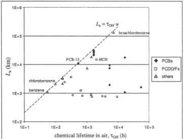
Fig. 3: Relationship between chemical lifetime in air, "COH, and the CTD in

air, /_., in the advective model. Depending on the difference between "CON and x a (determined by the stickiness of a chemical), deviations from the analytical relationship are obtained. For details, see Beyer et al. (2000)

= koH + F.ka,/h .. The factor F is the stickiness and is given by

F = ka~ ,/(kae s + ksffhs); ha g , g, is the height of the air, h, the depth of the soil compartment, kas and ksa are transfer velocities between soil and air and kaeg,, is the degradation rate in soil (Beyer et al. 2000). F is determined by partitioning coefficients, transfer velocities and the degradation rate in the non-mobile medium. This approach can easily be ex- tended to further media, e.g. water, sediment and vegetation. For F = 0, XOH is equal to "C a and in the L a vs. XoH plot

(Fig. 3), the chemical lies on the line defined by the analytical relationship L a = XoH-U. This behavior is observed for very volatile chemicals with a very low tendency to be adsorbed to and degraded in the soil, e.g. CFCs. If F > 0, the chemical lifetime XOH is greater than the atmospheric residence time x a and the point (XoH, L a) lies to the right of the line L a = ~oH.u. This is typical of less volatile chemicals re- maining in the soil after deposition, e.g. POPs.

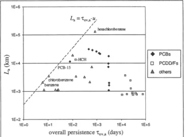
Again, a different relationship is obtained if the spatial scale is plotted versus the chemicals' overall persistence. The overall persistence depends on the p a t h w a y of release; here, we show the relationships between L, and the overall persistence after release to air, Xov, a , in the advective model, and between R a and the overall persistence after release to soil, ... in the closed dispersive model (Fig. 4 and 5). In the advective model, the overall persistence after release to air, x . . . . is related to the CTD by L a =

U'%va'ma/mtot

with m a

anal into t being the mass in air and the total mass. Thus, the fraction of the airborne chemical mass (which has to be calculated in addition to Xov, a from the multimedia model) determines the relation between the CTD and the overall persistence. The analytical relationships from Fig. 2 are shown by the dashed lines and, for some chemicals, the points (x .. . . La) and (%w, Ra) are indicated by dots and, in the case of aldrin, lindane and heptachlor (Fig. 5), by lines reflecting the uncertainty in the atmospheric degradation rates of these chemicals (Scheringer 1997). Similar to Fig. 3, the scatter of the points is caused by the differences between Xov,~ and "q. For m a n y chemicals, the following relationship between the different persistence measures holds: x a < '~OH < '[ov, a < 'lTov, s"

(5)

Long-Range Transport: Multimedia Fate Modeling

Review Articles

Fig. 4: Relationship between overall persistence after release to air, %v.a, and the C D T in air, La, in the advective model. Dashed line: analytical relationship from Fig. 2 (a). Dots: model results for different chemicals. De- pending on the difference between %,,a and "~., deviations from the analytical relationship are obtained. For details, see Beyer et al. (2000)

Fig. 5: Relationship between overall persistence after release to soil, "~ov,,, and the SR in air, R a, in the closed dispersive model. Dashed line: analytical relationship from Fig. 2 (c). Dots: model results for different chemicals. Depending on the difference between %~., and %, deviations from the analytical relationship are obtained. For details, see Scheringer et al. (2000a)

The different relationships in Fig. 2 to 5 show that "1~ a is the only persistence measure to which the spatial scale is directly related. (This relationship only holds if the air is the only mobile medium. If there are two or more mobile media, the degradation rates and flow velocities in these media in combination influence the spatial scale (Held 2001, Beyer and Matthies 2001)).

Dependent on the persistence measure chosen, different spatial-scale/persistence relationships are obtained. For a com- prehensive evaluation of the environmental fate of different chemicals, these different plots should be analyzed and compared. Since the spatial scale is determined by the interplay of various degradation and phase transfer processes, conclusions should not be drawn from a single measure and a single model. On the other hand, the Cqq) and SR are related to each other and show the same ranking of substances which made them favorable for the screening and prioritizing of chemicals.

4 Additional Factors and Open Questions

Determining the spatial scale of environmental chemicals is still impeded by a limited understanding of the relevant processes. Some important fields requiring further investigation are

9 The influence of aerosol particles on the degradability in air of semivolatile compounds. Adsorption to or absorp- tion into aerosol particles may decrease the degradation as compared to the gaseous state (Koester and Hites 1998, Harrad 1998) but it has also been hypothesized that it may increase the reactivity of the chemicals in some cases. In addition, it leads to increased deposition with the particles. All these factors influence the residence time in air and, thus, the spatial scale.

9 The effect of the influences of the t e m p e r a t u r e on degradability, phase partitioning (vapor pressure and Henry's law constant) and, in the case of semivolatile chemicals, adsorption to particles.

9 Lack of data and uncertainties in the physicochemical properties of many chemicals, e.g. water solubility, vapor pressure, Kow, K o o air-particle partitioning coeffi- cient. These uncertainties lead to considerable uncertainties in the m o d e l i n g results for spatial scale and persistence. Both improvement of data and uncertainty analyses of the models are required.

9 The influence of vegetation and ice and snow on the partitioning and degradation processes. If necessary, current models have to be modified so that they cover the effect of these media more appropriately.

9 The inclusion of transformation products, which is obvi- ously a necessary expansion of the assessment methods in such cases as DDT/DDE, aldrin/dieldrin, or heptachlor/ heptachlor epoxide. It is likely that there are additional cases in which transformation products are relevant. 9 The relationship to measurement data. For many chemi-

cals, the scarcity of measurement data makes it difficult to compare the modeling results with field data and to correlate the long-range transport potential indicated by a model with observed long-range transport.

Some of these questions will be addressed at a forthcoming OECD/UNEP workshop on 'Use of Multimedia Models in Screening PBTs/POPs for Overall Persistence and Long-Range Transport' to be held in October 2001 in Ottawa, Canada.

5 Screening Indicators in the Risk Assessment for Chemicals

With the help of models as described in this paper, different persistence measures and the potential for long-range transport can be determined for a variety of chemicals, and the chemicals can be ranked or grouped according to their exposure potential as expressed in terms of persistence (P) and spatial scale (S). Given the results of such an analysis, there are different ways of combining the results with hazard indicators for bioaccumulation (B) and toxicity (T). The more preventive approach is to label high-range chemicals as can- didates for replacement without extensive toxicity testing. The emphasis of this approach is to avoid widespread and long-term contamination. In a second step, only the remain- ing low-range chemicals are then tested for different types of toxicity, safety data such as inflammability, etc. In terms

(6)

Review Articles

Long-Range Transport: Multimedia Fate Modeling

of a PBT assessment (Snyder et al. 2000), this approach can be seen as a first filter that sorts out chemicals with a high P (and S and B), but without including the T dimension. T and other properties form the second filter.

The second, less preventive approach is to use a high persistence and potential for LRT as a trigger for priority toxicity testing so that the properties P (and S and B) and T are assessed in the first filter. This filter only sorts out chemicals with high P/S, high B, and high T.

In the comparison of these two approaches, a key question is how much and what kind of evidence of problematic environmental behavior is required for regulating a chemical. The current debate about the EU White Paper on chemical assessment (EC 2001) and about the role of the precautionary principle (Kristen 1999) indicates the need for further clarification of this issue.

6 Conclusions I n c o n c l u s i o n , w e s t a t e t h a t m e a s u r e s o f t h e s p a t i a l s c a l e c h a r a c t e r i z e t h e p o t e n t i a l f o r L R T o f a c h e m i c a l , t h a t t h e s p a t i a l scale is i n f l u e n c e d b y t r a n s p o r t a n d d e g r a d a t i o n p r o - c e s s e s in t h e d i f f e r e n t e n v i r o n m e n t a l m e d i a a n d b y a c h e m i c a l ' s p a r t i t i o n i n g b e t w e e n t h e s e m e d i a , a n d t h a t t h e s p a t i a l scale is r e l a t e d t o c o n c e r n s a b o u t i n t e r - r e g i o n a l fair- ness a n d equity. T h i s m a k e s t h e s p a t i a l scale a u s e f u l e x t e n - s i o n o f t h e i n d i c a t o r s c u r r e n t l y u s e d f o r c h e m i c a l assess- m e n t . D i f f e r e n t a p p r o a c h e s f o r d e t e r m i n i n g t h e spatial scale a r e c o n s i s t e n t w i t h e a c h o t h e r , b u t e m p h a s i z e d i f f e r e n t as- p e c t s o f t h e e n v i r o n m e n t a l m o b i l i t y o f c h e m i c a l s . T h e y p r o - v i d e a r e l i a b l e basis f o r t h e f u r t h e r i n v e s t i g a t i o n o f t h e v a r i - o u s f a c t o r s d e t e r m i n i n g t h e l o n g - r a n g e t r a n s p o r t p o t e n t i a l o f c h e m i c a l s in t h e e n v i r o n m e n t .

Acknowledgment. We thank A. Beyer and K. Fenner for technical sup-

port and helpful comments.

References

Bennett DH, McKone TE, Matthies M, Kastenberg WE (1998): General For- mulation of Characteristic Travel Distance for Semi-Volatile Organic Chemi- cals in a Multi-Media Environment. Environ Sci Techno132: 4023-4030 Bennett DH, Scheringer M, McKone TE, Hungerbiihler K (2001): Predict-

ing Long-Range Transport: A Systematic Evaluation of two Multimedia Transport Models. Environ Sci Technol 35:1181-1189

Beyer A, Mackay D, Matthies M, Wania F, Webster E (2000): Assessing Long-Range Transport Potential of Persistent Organic Pollutants. Environ Sci Techno124:699-703

Beyer A, Matthies M (2001): Long-Range Transport Potential of Semivolatile Organic Chemicals in Coupled Air-Water Systems. ESPR - Environ Sci Poll Res 8, this issue

Beyer A, Scheringer M, Schulze C, Matthies M (2001): Comparing Repre- sentations of the Environmental Spatial Scale of Organic Chemicals. Environ Toxicol Chem 20:922-927

Chapman P, Fairbrother A, Brown D (1998): A Critical Evaluation of Safety (Uncertainty) Factors for Ecological Risk Assessment. Environ Toxicol Chem 17, 99-108

EC (2001): White Paper - Strategy for a Future Chemicals Policy. COM (2001) 88 final. Brussels

Friscbe R, Esser G, Sch/Snborn W, KI6pffer W (1982): Criteria for Assessing the Environmental Behavior of Chemicals: Selection and Preliminary Quantification. Ecotox Environ Safety 6:283-293

Harrad SJ (1998): Dioxins, Dibenzofurans and PCBs in Atmospheric Aero- sols. In: Harrison RH, van Grieken RE (Eds): Atmospheric Particles. Chicbester: Wiley, 233-251

Held H (2001): Semianalytical Spatial Ranges and Persistences of Non-Po- lar Chemicals for Reaction-Diffusion Type Dynamics. In: Integrated Sys- tems Approaches to Natural and Social Dynamics (Eds Matthies, Malchow MH, Kriz J), Springer Heidelberg (in press)

Hertwich EG, McKone TE (2001): Pollutant-Specific Scale of Multimedia Models and Its Implications for the Potential Dose. Environ Sci Technol 35:142-148

Keeling CD, Heimann M (1986): Meridional Eddy Diffusion Model of the Transport of Atmospheric Carbon Dioxide 2. Mean Annual Carbon Cycle. J Geophys Res 91 D7:7782-7796

Klecka G, Boethling R, Franklin J, Graham D, Grady L, Howard PH, Kannan K, Larson R, Mackay D, Muir D, van de Meent D (2000): Evaluation of Persistence and Long-Range Transport of Organic Chemicals in the En- vironment: Guidelines and Criteria for Evaluation and Assessment. Pensacola: SETAC Press

Koester CJ, Hites RA (1992): Photodegradation of Polychlorinated Dioxins and Dibenzofurans Adsorbed to Fly Ash. Environ Sci Techno126:502-507 Korte F, Klein W, Drefahl B (1970): Technische Umwehchemikalien, Vor-

kommen, Abbau und Konsequenzen. Naturw Rdsch 23:445-457 Kristen C (1999): Precautionary Principle Challenges US Policy, Workshop

Finds. Environ Sci Technol 33: 304A-305A

Matthies M, Briiggemann R, Trenkle R (1986): Multimedia Modeling Ap- proach for Comparing the Environmental Fate of Chemicals. In: Envi- ronmental Modeling for Priority Setting Among Existing Chemicals (Eds GSF-Projektgruppe Umweltgef/ihrdungspotentiale von Chemikalien), ecomed publishers Landsberg, pp 211-252

Okubo A (1971): Oceanic Diffusion Diagrams. Deep Sea Res 18:789-802 Pekar M, Pavlova N, Gusev A, Shatalov V, Vulikh N, Ioannisian D, Dutchak

S, Berg T, Hjellbreke AG (1999): Long-Range Transport of Selected Per- sistent Organic Pollutants. EMEP report 4/99, Moscow: MSC-East Power M, McCarthy LS (1997): Fallacies in Ecological Risk Assessment

Practices. Environ Sci Technol 31: 370A-375A

Quartier R, MiiUer-Herold U (2001): On Secondary Spatial Ranges of Trans- formation Products in the Environment. Ecol Mod 135:187-198 Rodan BD, Pennington DW, Eckley N, Boethling RS (1999): Screening for Per-

sistent Organic Pollutants: Techniques to Provide a Scientific Basis for POPs Criteria in International Negotiations. Environ Sci Techno133:3482-3488 Rohleder H, Miinzer B, Voigt K (1986): E4CHEM (Exposure and Ecotoxicity

Estimation of Environmnetal CHEMicals) - A Computerized Aid for Priority Setting. In: Environmental Modeling for Priority Setting Among Existing Chemicals (Eds GSF-Projektgruppe Umwehgefiihrdungspoten- tiale von Chemikalien), ecomed publishers Landsberg, pp 491-524 Scheringer M (1996): Persistence and Spatial Ranges as Endpoints of an

Exposure-Based Assessment of Organic Chemicals. Environ Sci Technol 30:1652-1659

Scheringer M (1997): Characterization of the Environmental Distribution Behavior of Organic Chemicals by Means of Persistence and Spatial Range. Environ Sci Technol 31:2891-2897

Scheringer M, Berg M, Miiller-Herold U (1994): Jenseits der Schadensfrage: Umweltschutz durch Gef/ihrdungsbegrenzung. In: Berg M e t al. (Eds): Was ist ein Schaden? Ziirich: Verlag der Fachvereine, 115-146 Scheringer M, Wegmann F, Fenner K, Hungerbiihler K (2000): Investigation

of the Cold Condensation of Persistent Organic Pollutants with a Global Multimedia Fate Model. Environ Sci Technol 34:1842-1850

Scheringer M, Bennett DH, McKone TE, Hungerbiihler K (2001a): Rela- tionships between Persistence and Spatial Range of Environmental Chemi- cals. In: Lipnick RL et al. (Eds): Persistent, Bioaccumulative, and Toxic Chemicals II: Assessment and New Chemicals. Washington DC: Ameri- can Chemical Society, 52-63

Scheringer M, Held H, Stroebe M (2001b): Chemrange 1.0 - A Multimedia Transport Model for Calculating Persistence and Spatial Range of Or- ganic Chemicals. Ziirich, Laboratorium fiir Technische Chemie, httu:// |tcmail.ethz.ch/hungerb/research/product/chemrimge,ht;rnl

Snyder EM~ Snyder SA, Giesy JP, Blonde SA, Hurlburt GK, Summer CL, Mitchell RR, Bush DM (2000): SCRAM: A Scoring and Ranking System for Persistent, Bioaccumulative, and Toxic Substances for the N o r t h American Great Lakes. ESPR - Environ Sci Pollut Res 7:52-61 Wania F, Mackay D (1995): A Global Distribution Model for Persistent

Organic Chemicals. Sci Total Environ 160/161:211-232

Wania F, Mackay D, Li YF, Bidleman TF, Strand A (1999): Global Chemical Fate of Ix-Hexachlorocyclohexane. 1. Modification and Evaluation of a Global Distribution Model. Environ Toxicol Chem 18:1390-1399

Received: June 19th, 2001 Accepted: June 25th, 2001