Contribution to Efficiency Enhancement of Induction Motor Drive using Artificial Intelligence Techniques

2013/2014

Ministry of Higher Education & scientific Research

UNIVERSITY OF BATNA

FACULTY OF TECHNOLOGY

DEPARTEMENT OF ELECTRICAL ENGINEERING

LABORATORY OF PROPULSION SYSTEMS -

ELECTROMAGNETIC INDUCTION,LSP–IE,BATNA 2000

Contribution to Efficiency Enhancement

of Induction Motor Drive using

Artificial Intelligence Techniques

by

Zineb Rouabah

Electrical Engineer, University of Batna Master in Electrical Engineering,University of Batna A thesis submitted for the fulfillment of the degree of

Doctorate of Science in Electrical Engineering

Examining Committee

M.S. NAIT SAID Professeur University of Batna Président

F. ZIDANI Professor University of Batna –Rapporteur–

B. ABELHADI Professor University of Batna Co–Rapporteur–

K. SRAIRI Professor University of Biskra Examinateur

S. BENAICHA Lecturer A University of Sétif Examinteur

D. KERDOUNE S.CHAOUCH Lecturer A Lecturer A University of Constantine University of Batna Examiner Examiner

défluxage constitue un degré de liberté non exploité. Dans la plupart des cas ce degré de liberté est utilisé pour élaborer des stratégies de commande qui minimisent la consommation de l’énergie du moteur tout en respectant les spécifications du couple. Dans ce contexte les techniques

d’intelligence artificielles ont été largement exploitées dans le domaine de minimisation des pertes.

Parmi ces techniques l’application de la logique floue, les algorithmes génétiques, réseaux de neurones, technique PSO a montrée un degré de performance élevée dans le domaine de l’optimisation énergétique. Le présent travail entre dans ce cadre, où des algorithmes basées sur les techniques intelligentes : à savoir la logique floue et les algorithmes génétiques sont proposés pour optimiser le flux en ligne et par la même améliorer le rendement de l’ensemble motor asynchrone convertisseur statique, en tenant compte des pertes fer et de la saturation dans la machine. Les resultats obtenus attestent de l’efficacité des approches proposées aussi bien pour les faibles charges que pour les charges élevées. La robustesse de ces algorithmes fut aussi testée là aussi les résultats sont assez encourageants.

Mots clés : Moteur asynchrone, Onduleur, Contrôleur Flou , Algorithmes Génétiques Commande

Abstract

Acknowledgments Dedication

List of abbreviations List of tables and figures

Introduction 1

Chapter One

Artificial Intelligence Optimization Techniques

1.2 Artificial Neural Networks ...8

1.3 Particle Swarm Optimization (PSO) ...9

1.3.1. Original PSO Algorithm ...9

1.4 Fuzzy Logic System...11

1.3.1 Conventional and Fuzzy Sets ...11

1.3.2. Linguistic Variables and Values ...13

1.3.3. Membership Functions (MFs) ...13

1.3.4. Fuzzy Rules and Fuzzy Implication ...14

1.4. Fuzzy Logic Controller (FLC) ...15

1.4.1 Steps of Fuzzy Logic Controller Design ...16

1.4.2. Fuzzification Interface ...16 1.4.3. Rule Base...16 1.4.4. Inference Engine ...17 1.4.5. Defuzzification Inference ...17 1.6 Genetic Algorithms ...18 1.6.1 Implementation Details ...18 1.6.1.1. Selection ...19 1.6.1.2. Crossover ...20 1.6.1.3. Mutation ...20

1.7 Induction Motor Speed Regulation ...21

1.7.1 Speed Control using FLC 21

1.7.2 Optimizing an FLC using GA’s 24

Chapter Two

Motor and Inverter Losses Modeling

2.1. Introduction... 26

2.2.. Induction Motor Model including Saturation and Core Losses……….…….27

2.2.1. Simulation of the Motor Mode……….28

2.3. Inverter Model ...30

2.4. Pulse Width Modulation (PWM) ...31

2.5. Inverter Losses ...31

2.5.1 Inverter Conduction Losses ...31

2.5.2. Inverter Switching Losses ...32

2.6. Simplified Inverter Loss Model ...33

2.6.1 Simplified Model of Conduction Loss ...33

1.6.2 Simplified Model of Switching Loss ...33

2.7. Simulation of Simplified Inverter Model ...34

2.8 Summary 35

Chapter Three

Efficiency Optimization Approaches of Induction Machine Drive

3.2 Losses in Induction Motor Drives………..…… 37

3.2.1 Motor Losses Model……….………...…… 39

3.2.2 Losses Minimization……….……… 40

3.3 Proposed Loss Minimizing Strategies………..…… 42

3.3.1 Fuzzy Logic approach………...………...…… 43

3.3.1.1 First Fuzzy Approach……….………...………….…...…… 43

3.3.1.2 Second Fuzzy Approach………...……….………… 45

3.4 Genetic Algorithms Approach………..……… 48

3.5.1 Genetic Algorithms Optimization Procedure………...……… 49

3.5.1.1 Off Line Genetic Algorithms Optimization Procedure……….…… 50

3.5.1.2 On Line Genetic Algorithms Optimization Procedure………...…… 50

3.5 Results of GA’s application 51

Chapter Four

Simulation Results and discussion

4.1 Introduction……….. 53

4.2 Drive System………. 53

4.3 Simulation Results and discussion………. 54

4.3.1 Performance of Fuzzy Logic Approaches……….. 56

4.3.2 Performance of Genetic Algorithms ………. 58

4.4 Effect of Parametric variation on Performance of the Efficiency Optimization 60

4.4 1. Magnetic Saturation Effect ……….. 62

4.4 2. Efficiency Optimization of saturated IM……….. 63

4.4 3.rotor resistance Variation Effect On efficiency optimization……….. 67

4.4 Summary……….. 68

General Conclusion 69

References……… 70

I wish to express my sincere gratitude to my supervisors Pr F.Zidani and Pr

B.Abdelhadi, who have been a constant source of guidance, support and

encouragement throughout my Project .their extensive knowledge, rigorous

research attitude, diligent

working and creative thinking have inspired me and will definitely benefit my

career.

My gratitude should also be given to Pr . M.S. Nait Said , Pr K.Serrairi and

Doctors J.Kerdoune, S.Benaicha , S.Chaouch for serving as my committee

members, giving me valuable suggestions and taking the time to revise my

thesis. I would like to dedicate all my thanks to them.

Also I want to thank, Pr.F.Z. Louai, Pr R.Abdessemed, Pr. F.Nasri ,M

R.Amrani,

M

H.Nasri for their encouragement

To my mother memory

To my brother memory

• Rs , R_r stator and rotor resistance,

 Rfs , R_fr satorand rotor iron loss resistance,

• L s , L r stator and rotor leakage inductances,

• M magnetizing inductance,

 Ls total stator inductance,

 Lr total rotor inductance,

 σ leakage coefficient,

 σr rotor leakage coefficient

• Tr rotor time constant,

 ω motor speed,

 ωs synchronous speed,

 ωr

• Te , Tl electromagnetic and load torques,

• np number of pole pairs,

• J motor inertia constant,

• f coefficient of friction,

• v sd,v sq d and q components of the stator voltages,

• i sd ,i sq d and q components of the stator currents,

 rd, rq d and q components of the rotor flux linkages,

 i µ magnetizing current,

List of Abbreviations

 FOC Field Orientation Control

 LMC Loss Model Controller

 SC Search Controller

 GA’s Genetic Algorithms

 RCGA Real coded Genetic Algorithms

List of Figures and Tables

Chapter One : Artificial Intelligence Optimization Techniques

Figure 1.1. PSO Flowchart ... 10

Figure 1.2. Visualization of PSO Process ... 11

Figure 1.3. Temperature classification of a room on two sets ... 12

Figure 1.4. Typical shapes of MFs ... 14

Figure 1.5. Basic structure of FLC ... 16

Figure 1.6. Genetic Algorithms Flowchart ... 19

Figure 1.7. One-point crossover example... 20

Figure 1.8. Mutation example... 21

Figure 1.9. System step response ... 22

Figure 1.10. Inputs and output MFs of the induction motor speed control ... 23

Figure 1.11. Optimized inputs and output MFs of the induction motor speed control ... 24

Figure 1.12. Induction motor speed response ... 25

Chapter Two: Motor and Inverter Losses Modeling Figure 2.1. Equivalent circuit of the IM with series core loss resistance ... 27

Figure 2.2. Speed evolution ... 28

Figure 2.3. Torque evolution ... 29

Figure 2.4. Current evolution ... 29

Figure 2.5. Three phase inverter ... 30

Figure 2.6. Total inverter losses for one leg ... 33

Figure 2.7. Simplified Inverter Model ... 34

Figure 2.8. Inverter Losses v:a) current, b) switching frequency, c) modulation index,d) phase shift 34 Figure 2.9. Approximated Inverter Losses function ... 35

Chapter Three: Efficiency Optimization Approaches of Induction Machine Drive Table 3. 1 Rule matrix for efficiency improvement………... 44

Table 3. 2 Rule matrix for Kopt adaptation 47 Figure 3.1. Different types of losses in IM drives and possible methods for loss reduction……… 38

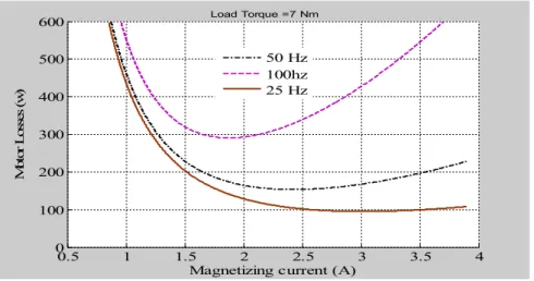
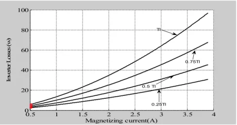
Figure 3.2. Total losses versus magnetizing current at nominal speed 41 Figure 3.3. Total losses versus magnetizing current at nominal load torque 41 Figure 3.4. Inverter losses versus magnetizing current 42 Figure 3.5. Block diagram of the Optimization Control System 42

Figure 3.7. The membership distribution………..… 44

Figure 3.8. The Optimization control law mapping………..… 45

Figure 3.9. The proposed Fuzzy controller………...… 45

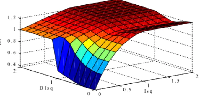
Figure.3.10 Kopt variation versus Ls ,M,Rrand Rs 46

Figure 3.11 The membership distribution 47

Figure 3.12 The Optimization control law mapping 48

Figure 3.13 Efficiency Optimization flowchart by genetic algorithms 49

Figure 3.14 Optimal solution obtained by genetic algorithms for TL=3.5Nm 51

Figure 3.14 Optimal evaluation obtained by genetic algorithms for TL=3.5Nm 51

Chapter Four: Simulation Results and Discussion Table. 4.1 Comparison of Energy saving for saturated and unsaturated Motor 65

Figure 4.1 Indirect vector Controlled IM with Efficiency Optimizer 54 Figure 4.2 Load Torque Profile and Torque response 55

Figure 4.3 Speed response 55

Figure 4.4 Motor Fluxes 55

Figure 4.5 Losses 55

Figure 4.6 Energetic performance of the drive 55 Figure 4.7 Fluxes of the motor 56

Figure 4.8 Energetic performance of the drive 57 Figure 4.9 Energetic performance of the drive 57 Figure 4.10 Efficiency Comparison for: high Speed (a) and low Speed (b) 58 Figure 4.11 Fluxes of the motor (a) RCGA approach, (b) off line Binary coding GA 58

Figure 4.12 Energetic performance of the drive: Losses (a) RCGA approach, (b) off line 59 Binary coding GA Figure.4.13 Energetic performance of the drive:Efficiency(a)versus time for a given profile load,59 (b) versus load Figure.4.14 Energetic performance of the drive: Losses ((a) RCGA approach, 59 (b) off line Binary coding GA Figure.4.15 Transit between transient and permanent mode 60 Figure.4.16 Saturated motor efficiency 61 Figure.4.17 Efficiency variation with parametric variation, 61

Figure.4.18 Performances of saturated IM , (a) Speed, (b) Torque, (c) Fluxes, (d) Stator inductance, 63 (e) Losses and (f) Efficiency Figure.4.19 Efficiency (a) First Fuzzy approach, (b) Kopt fuzzy approach,(c) RCGA ,(d) GA’s 64

Figure.4.20 Energy saving for (a) Saturated Motor, (b) Unsaturated Motor 66

Figure.4.21 Effect of Rr variation on fluxes 67

Introduction

The interplay between economic and environmental issues, increasing energy demand and limited resources, has driven efficiency improvement in every aspects of electrical engineering [Bazzi 2010]. More than 50% of the electrical energy produced worldwide is consumed by motors, mainly the three phase induction ones being the most widely used in industry application. The interest in energy saving is one of the major motivational factors in the introduction of variable-speed drives in some industries. Therefore, it is prevalent to encounter the efficiency computation for electric motors whenever variable-speed is considered, [R.Krishnan 2001]

Induction motors (IM) are imposing themselves as a reliable and more economical choice in a wide range of applications. In industry, they represent an important factor of control. The efficiency of a drive system is a complex function which depends on the type of the machine, the converter topology and the kind of semi conductor power switches and the modulation algorithm.

Furthermore, the control system has an important effect on drive efficiency. A drive system which normally operates at rated flux yields the fastest transient response. Depending on motor size and design, the rated load efficiency may attain 80 - 90% with power factors of 0.7-0.9. However, when the load is reduced, the performances degrade accordingly [Peter Vas 1999].

Power-loss minimization in induction machines has been investigated for over 30 years. The basic idea of efficiency optimisation control of motors is the adjustment of the motor flux go as to achieve a minimum loss and hence a maximum efficiency. Every motor operating point can be attained by different levels of motor flux and, usually, only one flux value among them ensures a minimum electrical loss. Efficiency optimizing controllers search this optimum value for each operating point and impose it to the machine under control. This leads to a maximum efficiency operation a whole load range [Jinchuan. Li ,.2005].

The IM efficiency optimisation of the drives can be realised by different types of loss minimisation strategies. There are basically two methods for efficiency optimization control: off-line and on-line methods. The off-line method calculates the flux of the motor at each operating point by a set of predefined mathematical equations. The resulting flux values for a range of operating points are then stored in a look-up table. During the motor operation,

the flux value, corresponding to the present operating point, is fetched from memory and is applied to the machine as a command variable. This method is fast and can be implemented easily, since the flux values either exist in memory or are calculated using a simple equation. However, it is very difficult, with this method, to take into account system parameter variations caused by factors like magnetic saturation of iron that affects motor reactance or changes in temperature which affects motor resistances [Jinchuan. Li et al 2005].

To overcome these limitations of the off-line method, on-line efficiency optimization control (loss minimization) has been proposed [S.Vaez , 1999], [N.uddin , 2007], [ S.Sergaki , 2008].

Review of Previous Works

Loss Minimization of Induction Motor Drives

Many drives operate at light load most of the time. At light loads, operation with rated flux causes excessive iron losses, thus reducing the efficiency of the drive. For these loads, the slip is small and only small rotor current can flow whitch result in increased magnetizing voltage , in consequent higher magnetizing current [Peter Vas,1999]. Therefore optimum efficiency at light load operation can be obtained by an appropriate selection of the flux. Although several papers dealing with the subject have been published Among those focused on the importance of saving energy the one of Nola [Nola, 1977] which proposed a power factor controller. He suggested energy could be saved at light load by restoring the balance between no-load losses and load losses. However limitation of this approach (load must be less than 0.45pu) was demonstrated [Lipo , 1983].

The first strategy of the efficiency optimal control was proposed by [Kusko , 1983]; it is based on an analytical model of losses for induction machine scalar control and direct current (DC) machines. An analysis of motor losses was presented and it is shown that for a given speed and load torque losses can be minimized by adjusting input voltage and frequency.

[Kirshen , 1985] proposed an optimal efficiency controller based on the finding of the minimum input power. Thus, by measuring the input power directly to the DC bus and using the vector control, they propose to gradually adjust the flux and torque stator current components until the input power reaches a minimum

*value for a given output power .It is obvious this strategy has the advantage to minimize the whole losses of the system drive and does not require. any knowledge of the model

parameters however it takes a long convergence time and generate torque ripples when flux value changes.

Loss Model Based Controller (LMC)

Among the techniques leading to efficiency improvement, the so called loss-model – based approach (LMC), which consists of computing losses by using the machine model and selecting a flux level that minimizes theses losses. It offers the advantage of fast response and no torque ripples . An overview of previous works is given hereafter.

In their work, [Kirshen., 1984] propose, as part of the design of a scalar control, a loss model much more developed introducing into account hysteresis and eddy currents losses by a resistance Rm. They also include in the equivalent circuit of the induction motor the stray losses. Their investigation also shows the importance of magnetic saturation in the loss model, thus making the optimal slip frequency load dependent and limiting the increase in air-gap flux for large loads.

[Kioskederis,l996] calculated the total of iron loss, copper and stray losses and derived the loss model controller to determine the optimal flux that minimizing the total loss of the scalar control of the induction motor drive. [P.Famouri,1991] derived the per unit efficiency of the IM as a function of slip, frequency and losses including the core loss, the copper losses, rotational power losses and power loss crossing the motor air gap. The optimal efficiency can be obtained at any operating torque and speed by calculating the optimal frequency.

In [Garcia., 1994] the authors propose a new version of the work of [Novotny., 1984], but based on vector control. The optimizing efficiency controller proposed by the authors includes a linear loss model but they did an analysis on the efficiency sensitivity to parameter variations. Parameter that has the greatest influence on the energy efficiency of the system was the rotor resistance Rr.

A loss model including magnetic saturation for machines with AC and DC was presented by [Bernal., 2000].

In [Chakrabotry, 2003],a hybrid method combining the loss model and the search approach was presented for the indirect vector control of IM to extract the best of both thus improved the speed and the adaptation capability for a possible change in load or parameters variation. However the computations of loss model and input power measurement have to

[S.Lim , 2004],developed a simplified loss model with leakage inductance. In this model loss was represented as a resistance connected to a dependant voltage source, the simulation and experimental results show that the loss calculation based on this simplified model was closer to that of full model of previous works.

[M.Nasir Uddin , 2008] presented an LMC based on induction motor model in d-q coordinates referenced to magnetizing current which leads to no leakage inductance in rotor. The obtained efficiency optimizer controller was implemented in vector control both simulation and experimental results show the effectiveness of the proposed method.

[C.C.De .Wit,1997] presented a procedure to get minimum energy by deriving the steady state values of current and fluxes for the given load and the design the steady state feedback control based on Lyaponov. Experimental results show good torque capability

One of the failing of LMC is that its precision depends on the accuracy of the motor drive and losses modeling. In the loss model development, a compromise between accuracy and complexity has to be found. To find the loss expression from the full model, it is a difficult task; this is why, in the majority of past literature review, motor models are taken with constant parameters which will lead to the LMC performances deterioration once these parameters are not constant anymore. The online estimation of these parameters can be the solution but it can make the whole minimization scheme more complicated to be implemented in real time [S.Vaez-Zadeh , 2005, [Sang Woo Nam,2006], [de Almeida ,2007]. To solve these issues, intelligent methods like Artificial Neural Networks, Fuzzy Logic,Genetic Algorithms, Practical Swarm Optimization (PSO) can be applied as their design does not require an exact mathematical model of the system and, theoretically, they are capable of handling any nonlinearity.

Search Controller (SC)

In [Sul and Park, 1988], a method that maximizes efficiency by means of finding optimal slip was proposed. The technique can be considered as an indirect way to reduce input power.

In [Sousa , 1995],the authors reduced the flux current reference by minimizing input DC bus power by using fuzzy logic nonetheless the torque pulsation is overcoming by feed forward pulsation torque compensation simulation and the experimental results demonstrate that the convergence time was accelerated. However this controller works only in steady state

when a change occurs in load or speed the control must returns to a nominal flux configuration which complicates the system implementation .Also [Bose, 1997] present a neuro –fuzzy version of the previous controller.

The work of [Sul., 1988] proposed an alternative approach to research based on the frequency of optimal sliding. the authors show that at a constant speed, performance

depends only on the slip frequency, regardless of the load torque. From voltage and stator

current, they deduce the slip frequency, torque and power input. Thus, for invariant load dynamic

time, they identify the optimal slip frequency of each operating point and placed it in memory. In normal operating mode, the control system has to adjust the frequency of optimal sliding previously identified.

In [G.S.Kim, 1992] the square rotor flux is adjusted until the measured power reached it minimum;the controller depends on rotor resistance and its variations is also taken into account. Three vector control schemes namely rotor flux orientation, stator flux orientation and air gap flux orientation was studied in [O.Ojo, I, 1993] for IM optimization of torque and efficiency and results shown that rotor flux orientation offers best optimal efficiency.

, [Murphy J.M.D, 1982].

LMC and SC Hybrid Strategy

Other researchers have combined the advantages of both techniques by proposing a hybrid strategy which combines fast convergence and robustness.

The developed controller in [S.N.Vulovasitc, 2003] ensures to retain good features of both LMC and SC, while eliminating their major drawbacks. Authors used input power to identify on-line the loss function parameters and optimize flux value. Parameters variation sensitivity and slow convergence were eliminated.

In [S.Ghozzi,K,2004],LMC and SC both was used and compared. The authors concluded that the LMC is more appropriate in Field Oriented Control (FOC) because the flux can be imposed in a short time while the SC vary the flux continuously which produces more torque ripples.

Artificial Intelligence Based Controller

In classical control systems, knowledge of the controlled system (plant) is required in the form of a set of algebraic and differential equations, which analytically relate inputs with

outputs. However, these models,are often complex, rely on many assumptions, contain parameters which are difficult to measure or may change significantly during operations and sometimes such mathematical models cannot be determined. Furthermore,dispite the great devoted efforts classical control theory suffers from limitations due to the nature of the controlled (linearity, time invariance etc..) These problems can be overcome by using artificial intelligence- based control techniques relaying on human motivated and procedures [Peter Vas, 1999].

There are many artificial intelligence (A I) based controllers applied to IM optimization through control using fuzzy logic (FL) or artificial neural network (ANN), Natureinspired algorithms,(NIA) like Genetic Algorithms (GA) and Particle Swarm Optimization (PSO) seem promising because of their social cooperative approach and also because of their ability to adapt themselves in continuously changing environment [C.Thanga Rag, 2009].

In the field of loss minimization,many works was performed in this area some of them are enumerate bellow:

[D.H.Kim, 2006] proposed a hybrid technique, GA-PSO based vector control of IM for loss minimization as well as torque control.

[L.Vuichard, 2006] presented fuzzy controller that enable to calculate the optimal flux value leading to efficiency improvement in short time. They use a linear model.

In [Peracaula,2002],a loss model including saturation was integrated in artificial neural networks (ANN). The response time of the efficiency optimized controller was about 100-120ms.

[E.Poirier,2001] derived the loss model by using genetic algorithms to find the optimal flux value. The convergence is very fast .The robustness of the algorithm for parameters variation, was demonstrated.

Problem Identification and Thesis Objective

As mentioned earlier, LMC is suitable for field oriented control but slacks of precision and depends on the accuracy of the motor drive and losses modeling.

To find the loss expression from the full model, it is a very hard task. In the most previous works motor model is taken with constant parameters then when they change the LMC

performance deteriorates. It is always a compromise between accuracy and complexity. Thus the objective of this thesis is to investigate the improvement of the system drive by optimizing energetic performance of IM drive. To perform this task intelligent techniques are introduced so as to make the efficiency optimizer controller derived from the loss model independent of or less sensitive to motor parameter change. In this thesis. the AI energy saving of Induction machine is presented. These AI comprises Fuzzy logic and Genetic Algorithms that are investigated and developed for this purpose.

Thesis Structure

After a general introduction to the undertaken work and the presented literature review, the main body of the thesis is structured as follows:

 Chapter one introduces the basic concepts, notation and basic operations for

artificial intelligent techniques such as .Fuzzy logic, genetic algorithms and

Particle Swarm Optimization that will be needed for efficiency optimization and control.

 Chapter two presents the induction motor model including iron loss and the

inverter loss model. The simplified inverter loss model will developed to be integrated in the efficiency optimization algorithm.

 Chapter three expresses losses which are involved in IM and methods used to

minimize them. The optimization is carried out by the use of the artificial intelligence methods described in chapter one.

 Chapter four describes the complete drive system including the developments

of the loss minimization algorithm. Extensive simulation results for both controller dynamics and loss minimization aspects will be presented.

 At the end, a summary of the contribution of this investigation to energy

saving with a general conclusion and proposed complementary future work are presented.

Chapter One

Artificial Intelligence Optimization Techniques

1.1 Introduction

From an engineering perspective, the description of artificial intelligence (AI) may be summarized as: “the study of representation and search through which intelligent activity can be enacted on a mechanical device”. This perspective has dominated the origins and growth of AI. The first modern workshop/conference for AI practitioners was held at Dartmouth College in the summer of 1956, [George F Luger,2005]

According to ), [D.A. Linkens, 1996]intelligent control shows high performance control over a wide range of operating conditions(e.g. parameters uncertainties) . It is defined as systems that have the ability to emulate human capabilities (planning, learning and adaptation). Unlike conventional control, intelligent control uses tow sources of information (learning from process and designer/skilled operator knowledge) to form the corresponding relationship between inputs and outputs. The most widely used intelligent control schemes are fizzy logic control (FLC), artificial neural networks (ANN). These techniques are used in the field of electrical drives for control process, estimation, system identification and optimization problems however genetic algorithms (GA’s) [Eldissouki, 2002] and particle swarm optimization are used to solving optimization problems.

There are two large electrical drive manufactures, which incorporate AI into their drives there are Hitachi and Yaskawa. In addition to this, Texas Instruments (TI) has built a fuzzy controlled induction motor drive using the TMS320C DSP. The main conclusion obtained by TI agrees with results obtained from various fuzzy-control implementations: the development time of the fuzzy-controlled drive is significantly less than the corresponding development time of the drive using classical controllers.SGS Thomson has also built some DC and AC drives incorporating fuzzy logic control, [P.Vas et al, 1996].

In all drives, but especially in electrical vehicles, energy is a crucial factor. However, by using AI it may be possible to improve the efficiency.

This chapter introduces the trends of intelligent control techniques and its application to AC drives for efficiency optimization. The study focuses on fuzzy control, genetic algorithms and PSO technique.

1.2 Artificial Neural Networks

Artificial Neural network (ANN) resembles human brain in learning through training and data storage. They can approximate complicated functions using several layers of neurons structured in a way similar to the human brain; so, ANN acts as a universal approximator. ANN has learning capability and generalization property. Because of its learning capability, ANN is very powerful in control applications where the dynamics of a plant or process control is partially known or the mathematical representation is very complicated. The generalization property is very useful because it allows training of the neural networks with a limited training data set.

Artificial neural network consists of a number of interconnected information-processing elements called neurons. It has certain performance characteristics in common with the biological neural networks, [Bose, 2006]. A neuron can be modeled to perform a mathematical function such as a pure linear function, step function, tan-sigmoid function etc. These neurons can be interconnected to establish a variety of network architecture. The attractive feature of the neural network is that it can be trained to solve complex nonlinear functions with variable parameters, which may not be attainable by conventional mathematical tools, [B.Kosko,1992]

1.3 Particle Swarm Optimization (PSO)

Particle Swarm Optimization is an evolutionary computation technique introduced in 1995; its idea is based on simulation of social behavior of animals such as bird flocks or fish schools

searching for food. PSO is another form of evolutionary computation it is population-based

method, like genetic Algorithm. However, the basic concept is cooperation instead of competition. It is also very similar to GA, but it does not have genetic operators.

In this algorithm, each individual is referred to as a particle and presents a candidate

solution to the optimization problem.Unlike other population-based methodologies, every

agent moves along its velocity vector, which is updated using two different best experiences; one is the best experience, which a particle has gained itself during the search procedure and the other is the best experience gained by the whole group. Combination of these experiences can provide useful information for each particle to explore new positions in the domain of the problem.

For each particle i, the velocity and the position of particles can be updated by the following equations, [Taher Niknam,2010 ]:

( + 1) = ( ) + 1 − ( ) + 2 − ( ) (1.1)

( + 1) = ( ) + ( + 1) (1.2)

Where i is the index of each particle, k is the discret time index, rand1 and rand2 are random numbers between 0 and 1.

Pi is. The best position found by ith particle, G is the global best particle among the entire

population.

The most used PSO algorithm form is including an inertia term and acceleration constants as, [Brian .Brige,2003] :

( + 1) = ∅ ( ) ( ) + [ 1 − ( ) ] + [ 2 − ( ) ] (1.3)

is an inertia function and α1,2 are acceleration constants.

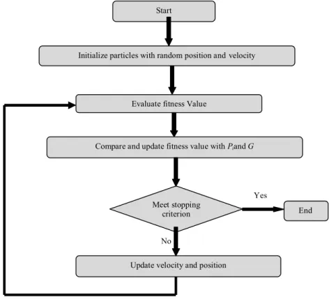
PSO optimization procedure is established according to the flowchart shown in Figure 1.1..

Fig( 1.1). PSO Flowchart

Yes Start

Initialize particles with random position andvelocity

Evaluate fitness Value

Compare and update fitness value with Piand G

Update velocity and position Meet stopping

criterion End

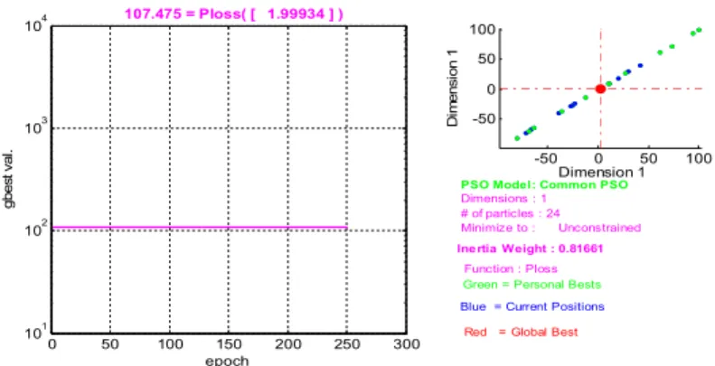
A simple example would be find the minimum of the loss function given in chapter three for

a given load Tl =25% TlN. A particle swarm optimization toolbox developed by [Brian

Brige,2003] was used obtained result is shown in Fig (1.2) bellow:

Fig( 1.2). Visualization of PSO process 1.4 Fuzzy Logic System

Fuzzy logic systems (FLSs) are else a universal function approximators. The heart of fuzzy logic system is linguistic rule-base, which can be interpreted as the rules of a single “overall” expert, or as the rule of “subexperts” and there is a mechanism (inference mechanism), where all the rules are considered in an appropriate manner to generate the output,[Zadeh,1965],[Mamdani and Assilian,1975],[Lee,1990] and [Kusko,1992]

Fuzzy logic control has found many applications. This is so largely employed because this fuzzy logic control has the capability to control non-linear, uncertain systems even in the case where no mathematical model is available for the controlled system.

The application of fuzzy logic has some advantages:

 When parameters change

 When existing traditional controllers must be augmented or replaced (e.g. to provide

self-tuning, to give more flexibility of controller adaptability, etc...).

 If sensor accuracy (or price) is a problem ( fuzzy logic can handle imprecise

measurements, uncertainties)

 To obtain solutions when solutions are not possible by using other technique.

1.4.1 Conventional and Fuzzy Sets

Fuzzy set theory resembles human reasoning in its use of approximate information and uncertainty to generate decisions. It was specifically designed to mathematically represent uncertainty and vagueness and provide formalized tools for dealing with the imprecision intrinsic to many problems.

-50 0 50 100 -50 0 50 100 Dimension 1 Particle Dynamics D im e n s io n 1 0 50 100 150 200 250 300 101 102 103 104 epoch g b e s t v a l. 107.475 = Ploss( [ 1.99934 ] )

PSO Model: Common PSO

Dimensions : 1 # of particles : 24

Minimize to : Unconstrained

Function : Ploss

Ine rtia Weight : 0.81661

Green = Personal Bests Blue = Current Positions

Within the framework of classical logic, a proposition is either true or false (1 or 0).to clarify this concept the example bellow is used:

For example, classical logic can easily divide the temperature of a room into two subsets, “less than 18° and 18° or more than 18°. Figure (1.2). (a) Shows the result of this partition. All temperatures less than 18 are then considered as belonging to the set “less than 18”. They assign a value of 1 and all temperatures reaching 18 or more are not considering as belonging to the set “less than 18”. They are assigned a value of 0.

However, human reasoning is often based on knowledge or inaccurate, uncertain or imprecise data. A person placed in a room in which the temperature is either 17.95° or 18.05°, will certainly distinguish between these two temperature values. This person will be able to tell if the piece is “cold “or “hot” without accurate temperature indication.

Fuzzy logic is used to define subsets, such as “cold” or “hot” by introducing the possibility to a value belonging more or less to each of these subsets.

( a) Two sets according to classic logic ( b) Two sets according to fuzzy logic

Fig (1.2). Temperature classification of a room in two sets

In fuzzy set theory, the concept of characteristic function is extended into a more generalized form, known as membership function: μA(x): U → [0, 1]. While a characteristic function exists in a two-element set of {0, 1}, a membership function can take up any value between the unit interval [0, 1]. The set which is defined by this extended membership function is called a fuzzy set. In contrast, a classical set which is defined by the two-element characteristic function, is called a crisp set, [M.N Cirstea et al, 2002]

According to the definition above a fuzzy set from Fig (1.2) can be defined as follows. Let U be a set, called the Universe of Discourse and u be a generic element of U (u ∈ ). A fuzzy set A in a universe of discourse U is a function that maps U into the interval [0, 1]. The fuzzy

set A is characterized by a membership function (MF) µA(x) that takes values in the interval

[0, 1]. µTemperature Temperature 0.5 cold hot 18 0.1724 0.1724 µTemperature 0.7066 Temperature 18 0.5 cold hot 0 1 1

1.4.2. Linguistic Variables and Values

Words are constantly used to describe variables in human’s daily life. Similarly, words are used in fuzzy rules to formulate control strategies. Referring to the above example, words like “room temperature is hot” can be used to describe the state of a system (in the current case, it is the state of the room). In this example, the words “cold” and “hot” are used to describe the variable “temperature”. This means that the words “cold” and “hot” are the values of the fuzzy variable “temperature”. Note that the variable “temperature” in its turn, can also take crisp values, such as 18°, 15.6°, 0°, etc.

If a variable is assigned some crisp values, then it can be formulated by a well established mathematical framework. When a variable takes words as its values instead of crisp values, there is no formal framework to formulate it in the classical mathematical theory. The concepts of Linguistic Variable and Value were introduced to provide such a formal framework. According to these concepts, if a variable can take words in natural languages as its values, then that variable is called Linguistic Variable. The words that describe the value of that linguistic variable are defined by fuzzy sets in the universe of discourse in which the

variable is defined [L.-X. Wang, 1997]. These words are called Linguistic Values.

In general a linguistic variable is characterized by (1) a name, (2) a term, and (3) a universe of discourse. For example on Figure 1.1. (b), the variable “temperature” is a linguistic variable with 2 linguistic values, namely “cold” and “hot”. The variable “temperature” can be characterized in the universe of discourse U = [-18°, +18°], corresponding to minimum and maximum temperature of the room, respectively. The linguistic values “cold” and “hot” can be characterized by the fussy sets described in Figure (1.2. b) or by any other set (depending on the application and the designer’s choice).

These definitions show that linguistic variables are the necessary tools to formulate vague (ill-defined) descriptions in natural languages in accurate mathematical terms. They constitute the first step to incorporate human knowledge into engineering systems in a

systematic and efficient manner, [L.-X. Wang, 1997].

1.4.3. Membership Functions (MFs)

There are many other choices or shapes of MFs besides the ones described in Figure (1.2). A graphical illustration of typical and commonly used ones in literature is shown in Figure 1.3., [K.M. Passino, 1998]

The simplest and most commonly used MFs are the triangular types due to their simplicity and computation efficiency,[ K.M. Passino, 1998],[Bose,2006]. A singleton is a special type of MF that has a value of 1 at one point on the universe of discourse and zero elsewhere. The L-function and sigmoid types are mainly used to represent saturation of variables.

Fig. (1. 3). Typical shapes of MFs (a) ..,(b) sigmoid,(c) L function,(d) Triangular,(e)

Gaussian function,(f) Trapezoidal,[M.N Cirstea, 2002]

1.4.4. Fuzzy Rules and Fuzzy Implication

A “fuzzy If-Then- rule” , also known as “ fuzzy rules”, “fuzzy implication”, or “fuzzy conditional statement” assume the form :

If x is A then y is B

Where A and B are linguistic values defined by fuzzy sets on universes of discourse X and Y, respectively. Often “x is A” is called antecedent or “premise”, while “y is B” is called the “consequence” or “conclusion”.

Examples of fuzzy if-then rules are widespread in our daily linguistic expression, such as the following:

 If pressure is high, then volume is small

 If road is slippery, then driving is dangerous

 If speed id high , then apply the brake is little

The expression “if x I A the y is B”, is sometimes abbreviated as →

The procedure for assessing these influences is called “Fuzzy Implication”. Since fuzzy propositions and relations are expressed by MFs, fuzzy implications also imply MFs as a method of interpretation.

In literature, there are a number of implication methods. The frequently used ones are

[BK.Bose 2002], [L.-X. Wang, 1997], [Z. Kovacic, 2006]:

1) Zadeh implication, 2) Mamdani implication, 3) Godel, implication, 4) Lukasiewicz implication, 5) Sugeno implication, 6) Larsen implication, etc

The differences between these methods are summarized in [Ajit.K.mandal.; 2006], [S.N.Sivanandam,2007], [Kwang.H.Lee,2005]. Their mathematical functions indicate that the Mamdani implication is the most suitable for hardware implementation, [ K.M. Passino, 1998]. It is also the most commonly used in control system applications.

1.5. Fuzzy Logic Controller (FLC)

Usually a control strategy and a controller itself is synthesized on the base of mathematical models of the object or process under control. The models of an object under control involve quantitative, numeric calculations and commonly are constructed in advance, before realization. Since fuzzy logic control is based on human knowledge and experience, it doesn’t need an exact mathematical model, it is an automatic control strategy based on “IF-THEN” rules.

The FLC can be viewed as a step toward a rapprochement between conventional precise mathematical control and human-like decision making.

The principal structure of a fuzzy controller is illustrated in Figure 1.3.. It consists of normalization factors, fuzzification of inputs, inference or rule firing, defuzzification of outputs, and denormalization.

Fig. (1.4). Basic structure of FLC 1.5.1 Steps of Fuzzy Logic Controller Design

 Initially choose the number of inputs/outputs

 Fuzzify the real inputs using appropriate membership functions

 Create the IF THEN rules using AND/OR operator

 Defuzzify the output fuzzy to get the corresponding crisp output

1.5.2. Fuzzification Interface

The fuzzification interface transforms input crisp values into fuzzy values and it involves the

following functions,[ Kwang H. Lee,2005].

 Receives the input values

 Transforms the range of values of input variable into corresponding universe of

discourse

 Converts input data into suitable linguistic values (fuzzy sets).

1.5.3. Rule Base

Although differential equations are the language of conventional control, the dynamic behavior of a system is characterized by a set of linguistic descriptions in terms of fuzzy rules in FLCs Fuzzy rules serve to describe the quantitative relationship between the input and the output variables in linguistic terms such that, instead of developing a mathematical model that describes a system, a knowledge-based system is used.

Rule Base Inference Engine Fuzzification (Input MFs) Defuzzification (Otput MFs) Denormalization Normalization

Fuzzy rules are the core of the FLC. Generally the dynamic behavior of a fuzzy controller is characterized by a group of fuzzy rules which follows the format:

If antecedents Then consequence.

The antecedents can be joined by union (OR) or by intersection (AND). In the speed control of induction motor for example typical rule reads as:

If “the speed error” is positive small (PS) AND “change in speed error” is negative small (NS) THEN u is negative small (NS).

1.5.4. Inference Engine

The function of the inference engine provides a way to translate the input of a fuzzy set into the fuzzy output. It determines the extent to which each rule is relevant to the current situations as characterized by inputs. The inference engine is the decision-making logic of an FLC. It has the capability of simulating human decision-making based on fuzzy concepts and inferring fuzzy control actions using fuzzy implication and the rule of inference in FL.

Normally this mechanism consists of set of logic operations.

There are several ways to implement a fuzzy inference: the Mamdani fuzzy reference system and the Sugeno reference system are two commonly used.[ Hung T. Nguyen.,2003]

1.5.5. Defuzzification Inference

The result of implication and aggregation steps in the inference engine is a fuzzy output. This output is the union of all the outputs of individual rules that are validated [Bose 2002]. The conversion of this fuzzy output set to a single crisp value (or a set of crisp values) is referred to as Defuzzification. Hence, this latter interface generates the output control variables as a numeric value.

Defuzzification can be implemented in different ways, general methods include MOM (mean of maximum), COA (center of area), and COM (center of maximum), [Hung T. Nguyen., 2003], [Bose, 2002].

1.6 Genetic Algorithms

Genetic algorithms (GAs) are global optimization techniques developed by John Holland in 1975. They are perhaps the most widely known type in the family of evolutionary algorithms,[Mitsuo. Gen, 2000]. These algorithms search for solutions to optimization

problems by “evolving” better and better solutions. A genetic algorithm begins with a

“population” of solutions and then chooses “parents” to reproduce. During reproduction, each parent is copied, and then parents may combine in an analog to natural cross breeding, or the copies may be modified, in an analog to genetic mutation. The new solutions are evaluated and added to the population, and low-quality solutions are deleted from the population to make room for new solutions. As this process of parent selection, copying, crossbreeding, and mutation is repeated, the members of the population tend to get better. When the algorithm is halted, the best member of the current population is taken as the

global solution to the problem posed,[Mitsuo.,Gen 2000],

[

Lee,2008];[Goldberg,1989].

There has been widespread interest from the control community in applying the genetic algorithm (GA) to problems in control systems engineering. Compared to traditional search and optimization procedures, such as calculus-based and enumerative strategies, the GA is robust, global and generally more straightforward to apply in situations where there is little or no a priori knowledge about the process to be controlled. As the GA does not require derivative information or a formal initial estimate of the solution region and because of the stochastic nature of the search mechanism, the GA is capable of searching the entire solution space with more likelihood of finding the global optimum.

The process of evolution is based on the following principles:

• Individuals in a population compete for resources and mates.

• The most successful individuals in each generation will have a chance to produce more

offspring than those individuals that perform poorly.

• Genes from ‘good’ individuals propagate throughout the population so that two good parents will sometimes produce offspring that are better than either parent. Thus each successive generation will become more suited to their environment.

1.6.1 Implementation Details

A population of individuals is maintained within search space for a GA, each representing a possible solution to a given problem. Each individual is coded as a finite length vector of

characters. A fitness value is assigned to each solution representing the ability of an individual to ‘compete’. The goal is to produce an individual with the fitness value close to the optimal. By combining information from the chromosomes, selective ‘breeding’ of individuals is utilized to produce ‘offspring’ better than the parents. Continuous improvement of average fitness value from generation to generation is achieved by using the genetic operators. The basic genetic operators are:

• Selection: used to achieve the survival of the fittest. • Crossover: used for mating between individuals. • Mutation: used to introduce random modifications.

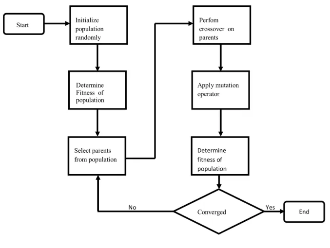
The genetic operators are used in the GAs optimization procedure according to the flowchart given in Figure (1.5).

Fig( 1.5). Genetic algorithms flowchart

1.6.1.1. Selection

The selection mechanism favors the individuals with high fitness values. It allows these

Initialize population randomly Perfom crossover on parents Determine Fitness of population Select parents from population Apply mutation operator Determine fitness of population Converged Start End No Yes

reproduction ability of least fitted members of population. Fitness of an individual is usually determined by an objective function.

1.6.1.2. Crossover

The crossover operator divides a population into pairs of individuals and performs recombination of their genes with a certain probability. If one-point crossover is performed, as shown in Figure (1.6)., one position in the individual genetic code is chosen. All gene entries after that position are exchanged among individuals. The newly formed offspring created from this mating are put into the next generation. Recombination can be done at many points, so that multiple portions of good individuals are recombined, this process is likely to create even better individuals. The crossover operator roughly mimics biological recombination between two single−chromosome (haploid) organisms.

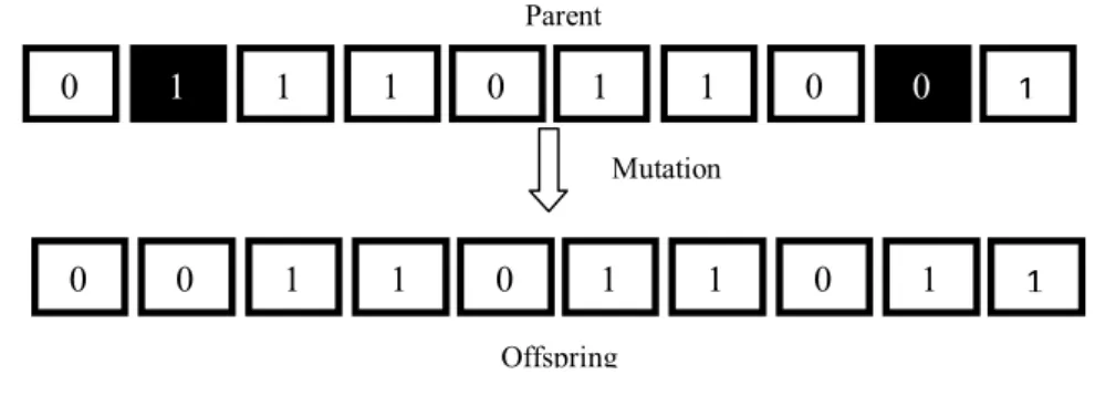
Fig (1.6). One-point crossover example 1.6.1.3. Mutation

When using mutation operator a portion of the new individuals will have some of their bits flipped with a predefined probability. In Figure (1.7). Mutation operator is applied to the shaded genes of the parent. The purpose of mutation is to maintain diversity within the population and prevent premature convergence. The usage of this operator allows the search of some regions of the search space which would be otherwise unreachable.

The described operators are basic operators used when the individuals are encoded using binary alphabet. Operators for real valued coding scheme were developed by Michalewicz [xx]. The following operators are defined: uniform mutation, non-uniform mutation, multi-non-uniform mutation, boundary mutation, simple crossover, arithmetic crossover and heuristic crossover.

• Uniform mutation randomly selects one individual and sets it equal to an uniform

random number. Parent 1 Parent 2 0 1 1 1 1 1 1 1 1 1 0 1 1 1 0 1 1 0 0 1 Crossover Offspring1 Offspring2

• Boundary mutation randomly selects one individual and sets it equal to either its lower or upper bound.

• Non-uniform mutation randomly selects one variable and sets it equal to a non uniform

random number.

• Multi-non-uniform mutation operator applies the non-uniform operator to all of the

individuals in the current generation.

• Real-valued simple crossover is identical to the binary version.

• Arithmetic crossover produces two complimentary linear combinations of the parents.

• Heuristic crossover produces a linear extrapolation of the two individuals.

Fig( 1.7). Mutation example

As an example of application of the two intelligent techniques used in this thesis an optimal fuzzy controller based on GA is developed in next section.

1.7. Induction Motor Speed Regulation

This section will be dedicated to investigate the speed regulation of IM using both techniques focused in this chapter mainly fuzzy logic and genetic algorithms, in the first step an FLC is used to regulate motor speed than it is performances are optimized by using GA’.

1.7.1 Speed Control using FLC

The components of the FLC will be introduced by using speed control of induction motor problem. Fig (1.9). depicts the typical response to step consign. One can see there are four zones:A1/ rise, A2/overtake,A3/ damping and A4/ steady state regions.

Offspring

0 0 1 1 0 1 1 0 1 1

Parent

Mutation

Fig. (1.8). System step response

Most closed-loop speed control systems react to the error (e (t)) between the reference speed and the output speed of the motor. When controlling processes, human operators usually compare the actual output of the system with the desired (reference) output and observe the evolution of this difference. This is why in most FLCs, including the controllers proposed in the input variables are the system error, e(t), and the change-in-error, Ce(t), to complete the initial description of the investigated speed control closed loop, let u(t) be the FLC output variable, i.e. the process input signal (which consist of the torque current

component namely Isq) .

As the first step is the fuzzification hence it:

(1) Measures the values of the input variables (e(t) and Ce(t) for the presented example, (2) Performs a scale mapping of the measured crisp values of the input variables into the

universes of discourse of these input variables, and

(3) Converts the input values into linguistic values compatible with the fuzzy set representation in the rule base. The three operations are performed as follows. Just as (e(t) and/or Ce(t)) take on values of, for example 0.2p.u at time instant t, linguistic variables also assume linguistic values at every time instant t. The values that linguistic variables take on over time change dynamically.

Let’s suppose, for the presented example, that e(t), Ce(t), and u take on the following values: “Negative Big” or NB, “Negative Small” or NS, “Zero” or Z, “Positive Small” or PS, and “Positive Big” or PB. The meanings of these linguistic values are quantified by their respective MFs. For close-loop speed control, each of the following statement quantifies some of different configurations of the system:

 The statement “e(t) is PB” can represent the situation where the output speed is

 The statement “e(t) is NS” can represent the situation where the output speed is just slightly over the reference, but not too close to it to justify quantifying it as Z and not too far to justify quantifying it as NB.

 The statement “e(t) is PB” and “Ce(t) is PS” can represent the situation where the

speed is significantly below the reference, but while “Ce(t) is PS”, the motor speed is away from its reference value.

These statements indicate that in order to fuzzify the dynamics of a process successfully, one must first have a good understanding of the physics of the underlying process. Moreover, the accuracy of the FLC is built on the shape, the number and the distribution of linguistic values or MFs used.

Figure (1.10). Shows the fuzzy sets and the corresponding triangular MF description of each signal. The universe of discourse of all the variables, covering the whole region and all the MFs are asymmetrical because near the origin (steady state), the signal requires more precision. This completes the first step of FLCs according to Figure (1.4)

. - 1 - 0 . 5 0 0 . 5 1 0 0 . 2 0 . 4 0 . 6 0 . 8 1 e ( t ) D eg re e o f m em b er sh ip N B N S Z P S P B - 1 - 0 . 5 0 0 . 5 1 0 0 . 2 0 . 4 0 . 6 0 . 8 1 C e ( t ) D e g re e o f m e m b e rs h ip N B N S Z P S P B - 1 - 0 . 5 0 0 . 5 1 0 0 . 2 0 . 4 0 . 6 0 . 8 1 u ( t ) D eg re e o f m em b er sh ip N B N S Z P S P B

1.7.2 Optimizing an FLC using GA’s

Many methods for fuzzy control use genetic algorithms to search the fuzzy controller structure or parameters. However, one of the drawbacks of applying genetic algorithms in optimal fuzzy controller design is a lack of the theoretical knowledge. Each application has a

different strategy to represent the fuzzy controller by chromosomes.

In this part; we will be interested by optimizing the MF’s of the speed controller used in section 1.3 to achieve this task the fuzzy controller ( MF’s plus normalization gains) formed the chromosomes while the fitness was the square error of the speed. Genetic operator parameters used probabilities of crossover and mutation are respectively set to 0.8 and 0.005.

Optimized MF’s obtained are shown in Figure (1.11). We can see that the MF’s intervals are changed compared with those in Figure (1.10).

- 1 - 0 . 5 0 0 . 5 1 0 0 . 2 0 . 4 0 . 6 0 . 8 1 C e ( t ) D eg re e o f m em b er sh ip N B N S Z P S P B - 1 - 0 . 5 0 0 . 5 1 0 0 . 2 0 . 4 0 . 6 0 . 8 1 e ( t ) D eg re e o f me mb er sh ip N B N S Z P S P B - 1 - 0 . 5 0 0 . 5 1 0 0 . 2 0 . 4 0 . 6 0 . 8 1 u ( t ) D eg re e o f m em b er sh ip N B N S Z P S P B

Fig(1.11). Optimized inputs and output MFs of the induction motor speed control

Figure (1.12). shows the obtained motor speed response for the reference speed of

157rad/s. Thus we can see that the optimized speed controller gives the best response

compared to IP and fuzzy controllers. Also it has a very fast perturbation rejection.

Fig (1.9). Induction motor speed response 1.8. Summary

This chapter has summarized the principles of some artificial intelligent techniques which are used to efficiency drives optimization. Attention has been focused on the two intelligent techniques investigated in this thesis namely fuzzy logic and genetic algorithms. The search of the IM speed response was investigated by both fuzzy logic and genetic algorithms to show the effectiveness of these two techniques.

The investigation of fuzzy logic and genetic algorithms in order to optimize efficiency of the induction motor drive is described throughout the next chapter.

0 0.5 1 1.5 2 2. 5 3 0 20 40 60 80 100 120 140 160 T im e (s ) S p ee d ( ra d /s ) R eferenc e F uzzy IP F uzzy-G A 1 .6 1. 8 2 2. 2 2. 4 2. 6 1 4 0 1 4 5 1 5 0 1 5 5 1 6 0

Chapter Two

Motor and Inverter Losses Modeling

2.1 Introduction

Induction motor is the most robust so the most widely used electrical machine, it is used in domestic, commercial and industrial applications. Being very economical, rugged and reliable, induction motors are used extensively and they consume a considerable percentage of the overall production of the electrical energy.

The motor parameters variation is often neglected when estimating motor performance, thus traditionally, the induction motor models are based on constant parameter model; however they do not give full satisfaction when flux level changes or increasing current

occur [E.Mendes et al, 1994].

In many applications like electric vehicles it is not only the high performances which are required but also the energy quantities must be optimal such the efficiency thus the flux level must change according to the operating point nevertheless the motor inductances cannot be considered constant. This change must be part of the calculations of the optimal conditions operating, because they have determinant influence on the optimum location and on the energy savings potential, [S.kirschen , 1984].

The induction motor can be connected directly to a standard fixed frequency, fixed voltage three phase power source. Under these conditions, the motor speed and slip will only be determined by the load torque. Power electronic converters are used to produce a variable-frequency supply to AC motors, thereby enabling variable-speed operations.

Power electronic converters have conduction and switching losses in the power devices, in addition to losses in both passive components and the auxiliary cooling systems. Therefore, modeling converters is a constant concern for electrical engineers, where various studies have been conducted in this area.

We can distinguish several approaches designed to represent either the fine development of electrical quantities or their mean values.

For the control of electrical machines, it is unrealistic to use fine representation of switching phenomena because it leads to prohibitive computational time. However in this project, a compromised solution is adopted from [Abrahamsen,2001] simplified model of the converter. This chapter is divided into two parts, the first one presents the mathematical model of the induction motor including iron losses and magnetic saturation , whereas the second one is dedicated to converter losses modeling.

2.2. Induction Motor Model including Saturation and Core Losses

A dynamic modeling of the IM has been widely studied in the literature, by using the famous Park transformation the six equations relating the stator and rotor voltages are reduced to four equations. This transformation is based on a set of hypothesis assumptions, among others symmetrical three phase machine and neglected saturation and iron losses.

The equations of stator and rotor voltages, and also the equation of motion can be used to express the system dynamics.

The magnetic saturation is generally including in the model by modeling the magnetizing inductance as a function of the magnetizing flux or current. Hence, the saturation can be modeled with a rather simple function and the resulting inductance estimate is accurate enough in most cases,[M.Ranta ,2013]

In order to take into account core losses and magnetizing saturation effects, Mendes’s and Razek model is used in this work.

In this model the iron losses are represented by an equivalent resistance in series with the magnetizing branch as represented on Fig. (2.1). they are given by the expression; while the saturation is taken into account by the piecewise [Mendes,.1994]:

= × + × (2.1) = 0.6 ≤ 0.8 . . > 0.8 (2.2)

Where: A and B and fs are respectively constants and stator current frequency.

Rs Vs Ls R’r/g (1-)Ls Rfs/1+r) Is Iµ Ir

Fig. (2.1) Equivalent circuit of the IM. with series equivalent core losses resistance

The choice of the state vector (Is Φr) allows us to neglect the cross saturation, without

great influence on results[Levi,1997] however the α-ß model for a three phase IM in the can be written, as ,[Z.Rouabah,2003]: r r fs r r s s s r r fs s s L R L M i L t d d i 1 R R V      _{ }              (2.3)





The electromagnetic torque is given by:





)

(

i

i

e

m

pM

C





The motion equation is given by the equation bellow:

− = + (2.6)

2.2.1. Simulation of the Motor Model

Simulation was performed using Matlab/simulink, for no load starting at nominal speed, obtained results are given bellow:

Fig. (2.2) Speed evolution

0 0.2 0.4 0.6 0.8 1 1.2 1.4 1.6 1.8 2 0 20 40 60 80 100 120 140 160 Time (s) S p e e d ( ra d /s ) linear model Iron loss Saturated model Iron Loss+ Saturation

0.4 0.42 0.44 0.46 0.48 0.5 0.52 0.54 0.56 115 120 125 130 135 140 145 150 155 160 165 Time (s) S p e e d ( ra d /s ) zoom

Fig. (2.3) Torque evolution

One can see on the above figures the influence of saturation on the torque which is subdued compared with the linear model however the speed rise time is greater than the linear model.

Figure(2.4) shows the current evolution it is clear that in startup the current value is high nevertheless in steady state this value decreases .

Fig. (2.4) Current evolution

0 0.2 0.4 0.6 0.8 1 1.2 1.4 1.6 1.8 2 -10 -5 0 5 10 15 20 25 30 35 40 time (s) T o rq u e ( N m ) linear model Iron Loss Saturated model Iron Loss+Saturation 0 0.2 0.4 0.6 0.8 1 1.2 1.4 1.6 1.8 2 -20 -15 -10 -5 0 5 10 15 20 Time (s) I s a lp h a (A ) iron loss saturation +iron loss Saturation linear model 0.7 0.705 0.71 0.715 0.72 0.725 0.73 0.735 0.74 0.745 0.75 -8 -6 -4 -2 0 2 4 6 Time (s) I s a lp h a (A ) zoom 0.42 0.44 0.46 0.48 0.5 0.52 0.54 0.56 0.58 0.6 -2 0 2 4 6 8 10 12 14 16 time (s) T o rq u e ( N m ) zoom