Background subtraction by disparity warping

Background Subtraction by Disparity Warping

by

John H. Liu

Submitted to the Department of Electrical Engineering and

Computer Science

in partial fulfillment of the requirements for the degree of

Master of Engineering in Electrical Engineering and Computer

Science

at the

MASSACHUSETTS INSTITUTE OF TECHNOLOGY

June 1998

@ John H. Liu, MCMXCVIII. All rights reserved.

The author hereby grants to MIT permission to reproduce and

distribute publicly paper and electronic copies of this thesis

document in whole or in part.

Author ...

Department

Certified by...

Engineering and Computer Science

A

22, 1998

Assistant Professor,

Aaron F. Bobick

MIT Media Laboratory

ThJsis Sup rvisor

Accepted by ...

...

.. .

...

Arthur C. Smith

Chairman, Department Committee onN(;i

ttden

ts

LIBRARIES

Background Subtraction by Disparity Warping

by

John H. Liu

Submitted to the Department of Electrical Engineering and Computer Science on May 22, 1998, in partial fulfillment of the

requirements for the degree of

Master of Engineering in Electrical Engineering and Computer Science

Abstract

In this thesis, I designed and implemented a background subtraction method based upon disparity verification that is invariant to run-time changes in illumination. Using two or more cameras, the method models the background by using disparity maps, which warp the primary image to each of the additional auxiliary images. During run-time, segmentation is performed by checking the color and luminosity values at corresponding pixels. When more than two cameras are available, segmentations be-come more robust and the occlusion shadows can generally be eliminated as well. The method assumes only fixed background geometry, which allows for illumination variation at run-time. And, because the three-dimensional reconstruction of the back-ground is performed during the off-line stage, the method is easily implemented to achieve real-time performance on conventional hardware

Thesis Supervisor: Aaron F. Bobick

Acknowledgments

I would first like to thank my thesis adviosr, Aaron Bobick, for making my time at the Media Lab a rewarding experience. His knowledge and insight has been invaluable to all of his students. I certainly am grateful to have the opportunity to work with him. Thanks to my academic Advisor, James Bruce, for helping my plan my courses and making sure I am on the right track.

Thanks to Anne Hunter, whose countless help on many occasions has made ev-erything run smoothly.

Thanks to Yuri Ivanov, who first came up with this cool idea and has helped me immensely ever since the beginning.

Thanks to Claudio Pinhanez, not only for the huge amount of time he spend giving me ideas, but also for the tremendous support he gave.

Many thanks go to the other HLV students - Chris Bentzel, Lee Campbell, Jim Davis, Martin Szummer, Stephen Intille, and Andy Wilson. Their friendship and fas-cinating conversations makes working fun. Special thanks to Chris, whose enthusiam and cheerfulness help smooth the tough times.

Thanks to all the faculty, support staff, and students of Vismod for making the environment great to work in. Special thanks to Kate Mongiat and Eric Trimble, both of whom made my life much easier in many ways.

Thanks to all my MIT friends, for making these five years memorable. You know who you are.

Thanks to all my SHS friends, who have helped me kept life outside of academics in perspective. And no, hopefully you don't have to send anymore "Earth to John" emails.

Special thanks to Vicky Yang, who has been my most supportive and understand-ing friend. Through good times and bad, I know I can always depend on you.

Last but not least, my thanks and love to my family. Mom, Dad, and David: without your support and love, I would never be where I am today. Thanks for everything and I am forever grateful.

Contents

1 Introduction 8

1.1 Im age Segm entation ... 8

1.2 M otivation . . . .... 9

1.3 Outline of Thesis . .. ... .. .. .. ... .. .. .. ... . 10

2 Previous Work: Background Subtraction 11 2.1 Sim ple Differencing ... 11

2.2 Motion-Based Segmentation ... .... 12

2.3 Geometry-Based Segmentation ... ... 12

2.4 Segmentation by Eigenbackground . ... 12

3 The Method 14 3.1 Building the Background Model ... 15

3.1.1 Data Collection .. ... .. .. . . . .. . . . 16

3.1.2 Interpolation ... 16

3.1.3 Refinem ent .. ... .. .. .. ... .. .... ... . 16

3.2 Subtraction . . . .. .. . 17

3.3 Removing the Occlusion Shadows ... . 19

4 Extensions 22 4.1 Models for Different Surfaces ... .... 22

4.2 Reducing Photometric Variations ... . . 23

5 Results 29

5.1 Lambertian Surfaces ... 29

5.2 Extreme Lighting Changes ... 30

5.3 Non-Lambertian Surfaces ... 33

6 Conclusion and Future Work 35

6.1 Improving the Method ... 35

A Delaunay Triangulation 37

List of Figures

3-1 Illustration of the subtraction algorithm. . ... . . 15 3-2 Occlusion shadow (a) Overhead view of the setting. (b) Pixel classified

as background. (c) Pixel classified as object. (d) Pixel also classified as object(occlusion shadow) ... ... .... .. 20 3-3 Removing occlusion shadow. (a) Middle and left camera pair classifies

the pixel as object(occlusion shadow). (b) Middle and right camera pair classifies the pixel as an occlusion shadow, and becomes background. 21 4-1 Sharp cornered edges. (a) The background from the view of the

pri-mary camera. (b) Same view after subtraction. . ... 23 4-2 Subtraction with different surface models. (a) The background from

the view of the primary camera. (b) Same view after subtraction using

different models ... 24

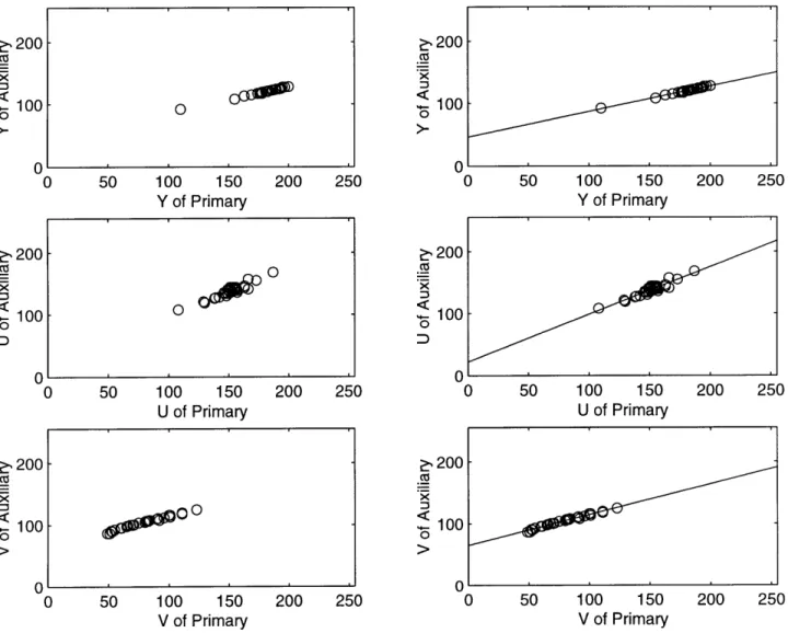
4-3 Polynomial fitting of the color warp. Top row: The Y component from the primary to the auxiliary camera. Middle row: The U component from the primary to the auxiliary camera. Bottom row: The V com-ponent from the primary to the auxiliary camera. . ... 25 4-4 Segmentation after color warp. (a) Primary camera view of the

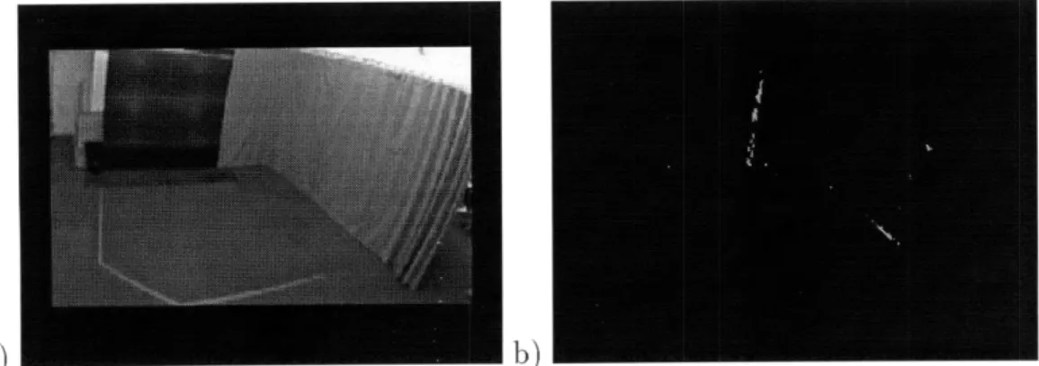
non-Lambertian surface. (b) Auxiliary camera view of the non-non-Lambertian surface. (c) Result without color warp. (d) Result with color warp. . 26

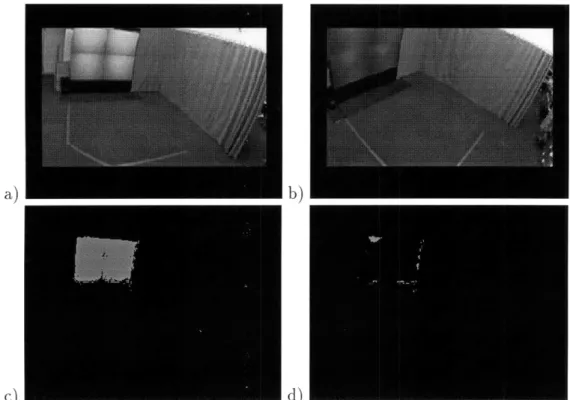
5-1 Two camera background subtraction. a) primary camera view of the empty scene, b) auxiliary camera view of an empty scene, c) primary camera view with a person in the scene. Bottom row: (d) results using simple tolerance range, (e) simple tolerance on refined disparity map, (f) windowed means on refined disparity map. . ... . 30 5-2 Three camera background subtraction. a) left auxiliary camera view,

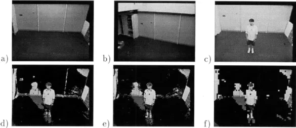
b) primary camera view, c) right auxiliary camera view, d) subtraction using views from a) and b), e) subtraction using views from b) and c), f) results of the removal of the occlusion shadow. . ... 31 5-3 Results of the algorithm during the computerized theatrical

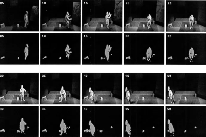
perfor-mance. The images show a sequence of ten video frames (1st and 3rd rows of images) , taken from a video five frames apart, and results of background subtraction by the proposed technique (2nd and 4th rows). Changes in lighting and background texture can be seen. . ... . 32 5-4 Best fit curves. The top row shows the fit for the Y component from

the primary to the first and second auxiliary camera. The middle row shows the fit for the U component from the primary to the first and second auxiliary camera. The bottom row shows the fit for the V component from the primary to the first and second auxiliary camera. 33 5-5 Enclosed room results with a person standing. (a) Primary camera

view. (b) First auxiliary camera view. (c) Second auxiliary camera view. (d) Subtracted image. ... 34 A-i Two ways of triangulation... . .. 37 A-2 Delaunay triangulation. (a) Triangulated figure. (b) A new point

is added to the figure. (c) An edge is flipped to maintain Delaunay triangulation . . . 39

Chapter 1

Introduction

When humans look at a photograph, the objects in the photograph are easily distin-guished. There is rarely any doubt about what is in the photograph, except in the case of visual illusions. When computers look at an image, everything in the image are simply a set of pixel values. Without further processing or additional information, nothing can be made out of what is in the image, much less the visual interpretation of action [1].

So how can one teach computers to identify objects in an image? That question has been around computer vision for as long as the field exists. But before one can find the solution to that question, one has to solve the question of how to segment out the important spots in the image that needs to be identified.

This thesis deals with a particular solution of that problem called background sub-traction. Specifically, we want to develop and implement a new method of background subtraction that works invariant of lighting conditions and texture changes.

1.1

Image Segmentation

In computer vision, image segmentation plays an important role in separating different groups of pixels into subsets united by their spatial relations. It is often one of the first steps in figuring out which parts of an image are useful to whatever applications the vision system is designed for. As stressed by [11], it is an important step for the

success of those vision systems. Without this step, applications such as tracking or classifying objects cannot be done.

This problem has been dealt with on a routine basis and has been implemented countless number of times by almost everyone who works in computer vision. The approach that is chosen is dependent on the nature of the scene as well as the param-eters which can be held invariant - lighting, color, spatial location, assumed surface properties, etc. It is a difficult problem, however, since variability of the environ-ments where computer vision finds its applications is extremely large. Therefore, the problem cannot be solved by one single approach for all cases.

Interestingly enough, biological vision systems in most cases have no problem doing segmentation. It is usually clear to us how to separate objects from the back-ground or from each other without thinking too much, if at all.

1.2

Motivation

Background subtraction is a form of image segmentation where the background is defined beforehand and any groups of pixels that do not belong to the predefined background should be segmented out as objects. While several approaches exist to deal with this task, few have the ability to deal with a background surface that

changes its texture, such as a projection screen or television.

While considering the solution to this problem, we realize that the property of being lighting dependent must also co-exist. The reason being that projection screens and televisions often emits its own light into the setting, which means that any vision systems that require calibration and run-time condition under very specific lighting will not work well since the lighting will be constantly changing.

With these two properties, applications such as computer theater comes to mind since they utilize settings where the lighting changes constantly to create moods and there are screens that are used as part of the background. This leads to the constraint in which the solution must be able to run in real-time in order to have computers interact instantly to an actor's actions. Therefore, the goal of this thesis is to develop

a new method of background subtraction that is invariant to both lighting conditions and texture changes, and at the same time is able to achieve real-time performance.

These three properties suggest a solution that only require the geometry of the background to remain static and uses two or more cameras. We create, during an off-line stage, disparity maps that warp the background from one camera to the other cameras. Segmentation is then performed during run-time by comparing color intensity values at corresponding pixels. Assuming the background is a Lambertian surface, if the pixel values match, then the background disparity is validated and the pixel is assumed to belong to the background. Otherwise, it is labeled as an object.

Because the basis of comparison is the background disparity warp between images taken at the same time, illumination or reflectance can vary without significantly affecting the results. And because most of the computational work of forming the disparity map is done during the off-line stage, the method will perform minimum number of computations during run-time to produce real-time performance.

1.3

Outline of Thesis

Chapter 2 presents various works related to solving the object segmentation prob-lem. Specifically, simple differencing, motion based segmentation, geometry-based segmentation, and eigenbackground.

Chapter 3 describes the method of background subtraction using the disparity maps. This chapter describes the off-line computations, the run-time computations, as well as how to refine the disparity maps.

Chapter 4 discusses some practical extensions that were used in conjunction with the method. The extensions include how to deal with non-Lambertian surfaces and recovery of the disparity maps due to accidental movements of the cameras.

Chapter 5 presents the results of the method when implemented for a couple of applications, including computer theater and tracking in an enclosed room.

Chapter 6 summarizes the whole experience and concludes with ideas for possible future work.

Chapter 2

Previous Work: Background

Subtraction

Previous attempts at segmenting objects from a predefined background have taken one of three approaches: simple differencing, motion-based segmentation, and geometry-based segmentation. The method presented in this thesis is most related to the last approach. In this chapter, I will discuss each of the three approaches, as well as a new approach that have recently arisen.

2.1

Simple Differencing

Simple differencing is the most commonly used approach for background subtraction. For example, in [16], the authors use statistical texture properties of the background observed over an extended period of time to construct a model image of the back-ground. The model is then used to decide which pixels in an input image do not belong to the background. This is usually done by subtracting the input image with the background model, and a pixel is declared to background an object if the differ-ence at that pixel is great than a specified threshold. The fundamental assumption of the approach is that the background is static in all respect: geometry, reflectance, and illumination.

2.2

Motion-Based Segmentation

This approach is based upon image motion. It presumes that the background is stationary or at most slowly varying, and that the objects are moving [4]. No detailed model of the background is required, but this approach is only appropriate for the direct interpretation of motion; if the objects are not moving, no signal remains to be processed. This approach requires constant or slowly varying geometry, reflectance, and illumination.

2.3

Geometry-Based Segmentation

The approach most related to the method presented in this thesis is based upon the assumption of static background geometry. [6] use geometrical constraints of a ground plane in order to detect obstacles on the path of a mobile robot. [13] employ special purpose multi-baseline stereo hardware to compute dense depth maps in real-time. Provided with a background disparity value, the algorithm can perform real-time depth segmentation, or "z-keying" [12]. The only assumption of the algorithm is that the geometry of the background does not vary. However, the computational burden of computing dense, robust, real-time stereo maps requires great computational power, as in [13, 12]. The method described in this thesis reduces the majority of the com-putational burden by modeling the background before run-time, so that no special hardware is needed for the implementation.

2.4

Segmentation by Eigenbackground

Based upon the assumptions of moving objects and static background, this approach uses an adoptive eignespace to model the background [14]. The model is formed by taking a set of sample images and computing their mean and covariance matrix. The latter is then diagonalized via an eigenvalue decomposition to create eigenvectors (eigenbackgrounds), which provide a robust model of the probability distribution function of the background. Using the mean and the eigenvectors, one can create an

image of the background and use the comparison from the simple differencing method to segment out the objects.

Chapter 3

The Method

The underlying goal of this thesis is to develop a new method background subtraction that utilize the geometrically static background surfaces. Since multiple cameras are used from different angles, we need to develop a stereo alogrithm that can reconstruct the model of the background.

What differentiates this method from the others is the idea that, for the purpose of background subtraction, we can avoid both the computation of depth and the reconstruction of the three-dimensional model of the background during run-time. The insight is that we can build a model of the empty scene off-line to avoid massive run-time computation. Now, during run-time, we only have to examine the incoming images and segment out the pixels that do not comply with this model. The stereo disparity map is used to model the background, and it serves the purpose of providing a simple and fast mechanism for the finding corresponding pixels in different images. The basic background disparity verification algorithm can be described as follows: For each pixel in the primary image,

1. Using the disparity warp map to find the corresponding pixel in the auxiliary image;

2. If the two pixels have the same luminosity and color (in YUV colorspace), then label the primary image pixel as background;

Figure 3-1: Illustration of the subtraction algorithm.

image either belongs to a foreground object, or to an "occlusion shadow" (to be explained in section 3.3);

4. If multiple cameras are available, then verify the potential object pixel by warp-ing to each of the other auxiliary image and lookwarp-ing for background matches.

For this algorithm to work, an accurate disparity map is required between the primary image and each of the auxiliary images, the background surfaces are assumed to be Lambertian, and the photometric variations between the cameras must be minimized. The algorithm is illustrated in figure 3.1.

The complete method consists of the three stages: computing the off-line dis-parity map(s), verifying matching background intensities, and eliminating occlusion shadows. We detail each presently.

3.1

Building the Background Model

The off-line part of the algorithm requires us to build a disparity map model of the background for each camera pairs. While traditional full stereo processing can be performed, it is not necessary in this case. Because the applications are typically indoor environments with large texture-less regions and because there is no compu-tational constraints, we use an active point-scanning approach to first get a robust sparse map. The map is then triangulated and interpolated to obtain a dense dispar-ity map. Furthermore, the map can be refined to reduce error. In detail, the three steps are:

3.1.1

Data Collection

In our case, we use a laser pointer to paint the background surface with easily de-tectable points. This can be done by turning off all light sources and set the computer to look for the brightest spot in its images. Since there should be no other light re-maining, the laser painted dots can be detected easily and accurately. Whenever a point is detected in both the primary and auxiliary images, we record its horiztonal and vertical disparities. This can be done for any number of arbitrarily selected sparse points, but usually the more points results in a more robust disparity map.

A problem occurs when an outlier has been included as part of the data. To avoid retaining the outlier, we manually detect its location and repaint the region surround it. The hope is that by doing so the outlier will be removed and be replaced with the

correct disparities.

3.1.2

Interpolation

After building the sparse disparity map using the method outlined above, we want to construct a dense disparity map by piecewise interpolation. To divide up the map into sets of triangular patches, we use Delaunay triagulation (explained in Appendix A) on the set of the measured points. Within each triangulation patch, we linearly interpolate the disparities.

3.1.3 Refinement

To compensate for errors that might have been introduced at each of the previous steps, an iterative procedure is used to refine the interpolated disparity map by first using that map to get an approximation of the corresponding location of a pixel from the primary image in the auxiliary image. Then a small neighbor search is performed to find the best local match. This location of the new best match becomes the new disparity.

3.2

Subtraction

During run-time, the subtraction algorithm warps each pixel of the primary image to the corresponding pixel auxiliary image using the disparity map built during the off-line stage. The pixels are then compared to see if their luminosity and color, YUV, values matches. We choose YUV versus other colorspaces such RGB because YUV explicitly models the separation between intensity (Y) and color (UV).

Let r be a coordinate vector (X, y) in the primary image I, and let r' be a vector of transformed coordinates (x', y') in the auxiliary image I'. Then we define the following variables:

r = (x, y) position in primary image I(r) primary image pixel Dx (r) horizontal disparity

DY(r) vertical disparity

r'= (c', y') position in auxiliary image ' = x - DX(r) x position in auxiliary image y= y - DY(r) y position in auxiliary image

i'(r') auxiliary image pixel

where vector I(r) consists of the YUV components of the pixel. Next we define a binary masking function m(I(r), I'(r')) for the construction of the background sub-tracted image. This masking function determines the complexity and accuracy of the algorithm.

In the deal scenario, we can define an extremely simple masking function to be a test to see if the corresponding pixels between the primary and the auxiliary images are exact the same. So here, we define m(I(r), I'(r')) to be:

m(I(r),I'(r')) 0 if (r) = I(r') (3.1)

1 otherwise

However, that never happens because usually there is still a slight photometric vari-ation between the cameras or the measurements simply are not that accurate to

permit this strong comparison. Therefore, we relaxed the constraint to compensate for potential errors and redefine m(I(r), I'(r')) to accept a value within some tolerance range:

m(I(r), I'(r')) 0 if (r) - (r < (3.2) 1 otherwise

Along with this straightforward method of subtraction, we have implemented a more robust, sub-sampling method which performs subtraction over a small neigh-borhood of a pixel. This technique introduces the least amount of interference with the normal computations, giving the advantage of being more forgiving about the precision of the disparity map. We partition the original primary image into a grid of small windows and compute a mean of each window of the grid. Next we warp the pixels of each window of the primary image into the auxiliary image and compute the mean of the resulting set of generally non-contiguous points. We then compare the means by the same procedure as above. For a k x k window of pixels in the primary image Wi,, the window mean images are computed as:

1

I;j = k2 I(r) (3.3)

Sx,yEW,_

1

SI'(r') (3.4)

where Wj is the set of auxiliary image pixel locations to which the pixels in the primary image window were warped. N in the second equation denotes the number of pixels in the auxiliary image that after warping remained inside the auxiliary image boundaries. The masking function is defined as:

0 if

11ii

-

Ij

<

m(I(r),I'(r')) = x,y E Wij; x', y' E Wj (3.5) 1 otherwise

which yields a blocked (or, equivalently, sub-sampled) background subtracted image. The proposed algorithm is simple and fast enough for real time performance. It is as fast as the conventional image differencing routines used, for example, in [9] in that each pixel is only examined once. One obvious advantage is that in using disparity for identifying a candidate background, we can accommodate for changing textures and lighting conditions. The algorithm effectively removes shadows and can be modified to remove surfaces selectively.

3.3

Removing the Occlusion Shadows

The occlusion shadow is a region of the primary image which is not seen in the auxiliary camera view due to the presence of the actual object. The creation of occlusion shadow is shown in figure 3.2. In figure 3.2 (a), we see an overhead view of the primary and auxiliary cameras views, as well as black object in front of a white wall. In figure 3.2 (b), the cameras finds the corresponding pixels of a point on the wall, which is then labeled background since the pixels are both white. In figure 3.2 (b), the primary camera sees black while the auxiliary camera sees white, so the pixel is labeled object. Now in figure 3.2 (c), the situation is reversed: the primary camera sees white while the auxiliary camera sees black, and the pixel in the primary image is also labeled object. However, according to our knowledge, the pixel in the primary image actually should be background. An Occulsion shadow is the group of pixels that are labeled objects as a result of the situation shown in figure 3.2 (c).

Intuitively, the occlusion shadow is of the same shape as a normal shadow that would be cast by the object if the auxiliary camera were a light source. The idea to solve this problem is based on that intuition. We can remove the occlusion shadow in the same manner as we would remove the regular lighting shadows: "illuminate" the occluded pixels by an additional auxiliary cameras. If multiple cameras are available, we can verify the potential object pixels by warping to each of the other auxiliary images and looking for background matches. For a given pixel, "the "real" objects will fail the disparity test in all camera pairs, whereas the shadow will typically only

White Wall I I Black Object Auxiliary Primary Camera Camera Object Background I E

Object (Occlusion Shadow)

Figure 3-2: Occlusion shadow (a) Overhead view of the setting. (b) Pixel classified as background. (c) Pixel classified as object. (d) Pixel also classified as object(occlusion shadow).

Object (Occlusion Shadow)

a) W W b)

Figure 3-3: Removing occlusion shadow. (a) Middle and left camera pair classifies the pixel as object(occlusion shadow). (b) Middle and right camera pair classifies the pixel as an occlusion shadow, and becomes background.

fail in only one. This is shown in Figure 3.3. Now that there is a second auxiliary camera, the second pair can verify whether or not the first camera's result is truly an object or simply an occlusion shadow.

If there are multiple objects in a scene, then it is possible for accidental alignment

to cause an occlusion shadow to be shadowed in every auxiliary image, which would be mistakenly labeled as object. Additional cameras can mitigate this effect.

Chapter 4

Extensions

The segmentation method, as described in Chapter 3, can be implemented straight-forwardly and used without change in some instances. However, there are exceptions in which additional work must be added to maintain the success of the model. In particular, the two situations that often arise to disrupt the ability of the model are non-Lambertian background surfaces and the accidental movement of the cameras. We deal with these situations by defining methods to reduce photometric variations and adjust the disparity maps. Also, surfaces connected at a sharp angle often cause the edge in-between to be incorrectly interpolated. The solution to this is to model the disparity maps separately for each surface and then combining them into a single disparity map just before run-time.

4.1

Models for Different Surfaces

During the course of building and testing the disparity maps, it becomes apparent that problems often exist when interpolating between the edge of two sharply connected surfaces, such as a wall and a floor. Because the disparity map must be as precise as possible, the interpolation of the disparity at the edge is often not accurate enough due to the limitation of how close the laser pointer can be pointed to it. This makes the edge between two sharply angled surfaces very hard to subtract out. Often, a sharp line appears at where the edges are, as in the case with figure 4.1.

a) b)

Figure 4-1: Sharp cornered edges. (a) The background from the view of the primary camera. (b) Same view after subtraction.

An unrelated problem that occurs is that sometimes a small part of the disparity map is incorrect and needs to be fixed. Given the current model, the only way to correct this situation would be to rebuild the entire disparity map. That is often very time-consuming, especially given that only a small portion of the map is incorrect.

One solution to both of these problems is to divide the background into multiple surfaces. Each surface would be defined by a mask and has its own disparity map. This would help solve the edge problem because there is no interpolation done at the edges. Each surface is interpolated with respect to itself and the points along the edges are simply the combination of the two connected surface, instead of the smooth interpolation between the two. At the same time, because the disparity maps are built separately for each surface, they can be rebuilt individually as well. This way surfaces with good disparity maps do not need to be subject to the risk of outliers nor the time-consuming effort of being rebuilt due to mistakes in other surfaces. The

result for this is shown in figure 4.2 below:

4.2

Reducing Photometric Variations

The success of the background subtraction method, as described in Chapter 3, relies on the assumption the background contain only surfaces that are Lambertian. An ideal Lambertian surface is one that appears equally bright from all viewing directions and reflects all incident light. However, there are times when parts of the background

a) b)

Figure 4-2: Subtraction with different surface models. (a) The background from the view of the primary camera. (b) Same view after subtraction using different models.

contain surfaces that are not Lambertian. For these surfaces the light emitted falls off at a very sharp rate. The result is that these surfaces tend to appear darker when viewed from more oblique angles [7]. This is problematic because now the same surface creates different image intensities when viewed from different directions. Therefore, our assumption of the Y, U, and V direct correspondence between the cameras are broken and the method cannot segment out these surfaces correctly.

To deal with this effect, we must adjust our data for the photometric variations between the cameras. The problem can be solved by modeling the YUV mapping from the primary camera to each of the auxiliary cameras. To accomplish this, we collect dozens of sample images for each camera while viewing the non-Lambertian surface as it displays uniform colored patches. The data for each color is then averaged by the number of pixels in the camera image. Since the goal is to find a best fit where the sum of the squared error of the segmentation are minimized, the data points for each main-auxiliary camera pair are used to obtain a least squares curve fitting to a polynomial.

The result of this experiment shows that a simple linear model fits the training data set well for most cases, and often the model can be used for the entire surface without variation for individual pixels. We allow linear photometric correction pa-rameters to be indexed by image location, defining different maps for different image regions. We assume the effect is insensitive to color, and use the same map for Y, U, and V.

50 100 Y of 150 200 250 Primary 50 100 150 200 250 U of Primary 50 100 150 V of Primary 200 250 200 100 > , 200 x S100 0 o >. 100 150 Y of Primary 200 C 100 Z) 50 100 150 U of Primary 200 250 200 250 0 50 100 150 200 250 V of Primary

Figure 4-3: Polynomial fitting of the color warp. Top row: The Y component from the primary to the auxiliary camera. Middle row: The U component from the primary to the auxiliary camera. Bottom row: The V component from the primary to the auxiliary camera. , 200 -x CO S100 o >-0 0 Cd x < 100 0 0 - 0 0 200 -100 I | I ! i i I 000 O0

a) b)

c) d)

Figure 4-4: Segmentation after color warp. (a) Primary camera view of the non-Lambertian surface. (b) Auxiliary camera view of the non-non-Lambertian surface. (c) Result without color warp. (d) Result with color warp.

A situation where this problem arises in one of our applications is when the back-ground contained a rear-projection screen. The result of that polynomial fitting is shown in figure 4.3. As stated above, the polynomial turns out to be linear for all Y, U, and V components.

We warped the values from primary camera through the linear model that we obtained to a new set of values. Then we used these values and the values from the auxiliary camera for segmentation comparison. The result is shown below in figure 4.4. Figure 4.4 (c) displays the segmenting of the projection screen from figure 4.4 (a) and figure 4.4 (b) without the color warp, while figure 4.4 (d) displays the segmenting using the color warp.

4.3

Fixing the Disparity Map

Though the description of how to build a disparity may sound simple, in practice, it can be a rather time-consuming process depending on the number of types of surfaces contained in the background. Although we can use various methods to keep the cameras stationary, often times it is difficult to maintain their precise positions -the disparity map calibration - for an extended period of time. For example, in [15], on several occasions spectators accidentally moved one of the cameras, and caused progressive deterioration of the quality of the subtraction.

To accommodate this situation, we developed a technique that recovers the dispar-ity map if only one camera has been moved. Here the assumption is that the camera only moves slightly so that the result is an affine transformation of the disparity map, which we need to estimate. Let A be the unknown affine transformation matrix. ra, the new position in the disparity maps D and DY , is now defined by:

ra = A

where i is an augmented coordinate vector i = (x, y, 1)T. Collecting all the terms into a parameter vector 0, we can reformulate the problem as an optimization problem, where the cost function is the sum squared error computed over all the pixels of the image:

Eo = [I(r) - I'(r')]2 (4.1)

In appendix B, we arrive at the final gradient descent equation:

E [I(r) - I'(r')] VI'(r')VD(Ai)C(r) = 0 (4.2)

Xy

where

VD(Ai)-- VD(ra)

VDr(r)

As it turns out, the gradient descent function does not work well when the initial guess about the matrix is far from the optimal transformation. There are several standard techniques that allow for improvement of the descent routine. One solution is to slightly blur the images, which allows the initial parameters to be farther away from the optimal ones. Other possible approaches are to employ multi-scale optimization or a stochastic gradient descent.

Chapter 5

Results

The method for background subtraction using disparity warp has been tested using various types of background. Against Lambertian surfaces, the algorithm presented in Chapter 3 can be used directly. Against extreme lighting conditions, additional modeling must be added to take care of special cases that do not exist otherwise. Against a non-Lambertian surface, the extensions in Chapter 4 must be added to successful remove the surface. This section will presents the performance of the method under these different situations.

5.1

Lambertian Surfaces

The results of the background subtraction methods on Lambertian surfaces are shown in figure 5.1and 5.2. The wall and the floor are the only surfaces that were modeled as part of the background, so other objects in the scene also are segmented besides the person.

Figure 5.1 demonstrates the background subtraction method using two cameras. The first pair of images, Figure 5.1 (a) and 5.1 (b), show camera views of an empty scene. Figure 5.1 (c) shows the primary image at run-time with the person in the view of the camera. Figure 5.1 (d) shows the background subtracted using a simple tolerance range . Figure 5.1 (e) shows the results of background subtraction using a simple tolerance range after the disparity map has been adjusted by the refinement

a) b) c)M

d) e) f)

Figure 5-1: Two camera background subtraction. a) primary camera view of the empty scene, b) auxiliary camera view of an empty scene, c) primary camera view with a person in the scene. Bottom row: (d) results using simple tolerance range, (e) simple tolerance on refined disparity map, (f) windowed means on refined disparity map.

procedure. Figure 5.1 (f) shows the windowed means on a refined disparity map. Note the presence of the occlusion shadow right behind the person in the last three images.

Figure 5.2 demonstrates the process of removing the occlusion shadow. The views of the three cameras are shown in the top row, where figure 5.2 (a) represents the left auxiliary camera, Figure 5.2 (b) represents the primary camera, and figure 5.2 (c) represents the right auxiliary camera view. Figures 5.2 (d) and 5.2 (e) show subtraction performed on two pairs of images. Finally, Figure 5.2 (f) shows the result of using all three cameras. Note the removal of the occlusion shadow when using multiple cameras.

5.2

Extreme Lighting Changes

The method for background subtraction using disparity warp was implemented as part of "It/I"'s vision system. "It/I" is a computerized theatrical performance in which computer vision was used to control a virtual character which interacted with a human actor on stage [15]. During the performance, theatrical lighting and projection screens are both used, which presents a problem for traditional segmentation techniques but

a) M b) c)

d) e)

f)

Figure 5-2: Three camera background subtraction. a) left auxiliary camera view, b) primary camera view, c) right auxiliary camera view, d) subtraction using views from a) and b), e) subtraction using views from b) and c), f) results of the removal of the occlusion shadow.

not for this method.

On top of the regular implementation of the method described in Chapter 3, there are situations where additional modeling are required. In particular, the extreme lighting conditions force us to add additional constraints to our models. For example, sometimes high light intensity leads to saturation of regions in the image. In those regions, the pixels provide no useful color (i.e. U and V) information since they are "washed out". Another example is when the lighting is so low that it falls below the cameras' sensitivity and provides information for neither intensity nor color.

For these special situations simple modifications to the original masking function was used. The modifications are easy to implement in YUV color space. For the first case, we added the constraint where if the value of the Y component is above some threshold value Ymax, we based the comparison II(r) - I'(r') < c only on the Y component of the vector. For the latter case, if the value of the Y components falls below some sensitivity threshold Ymin, the pixel is automatically labeled as

... .... ... .... ... Aj "IA 'A 3 S ININ 35 40

Figure 5-3: Results of the algorithm during the computerized theatrical performance. The images show a sequence of ten video frames (1st and 3rd rows of images) , taken from a video five frames apart, and results of background subtraction by the proposed technique (2nd and 4th rows). Changes in lighting and background texture can be seen.

background without further comparisons. Finally, for all other values of Y, equation 3.2 is used as given.

The projection screen turns out to present little problem because the cameras are all so far away and the viewing angle between them are not far apart enough to treat it as a non-Lambertian surface. We simple have to increase the tolerance range C for the projection screen in order to subtract it out correctly.

The results of the modified algorithm are shown in figure 5.3. The disparity-based background subtraction method is effective in compensating for dramatic changes in lighting and background texture. In the sequence presented in the figure, the lighting changes in both intensity and color. The starting frame shows the scene under a dim blue light. In a time interval of about two seconds the light changes to bright warm

c 200 100 0 100 C >-_{c 20C} x ce 0 50 100 150 200 250 U of Primary 50 100 150 200 250 V of Primary 50 100 150 Y of Primary .5 200 100 6-0 0 100 0 0 . 200 C: 100 "0 0 200 250 200 250 0 50 100 150 200 250 V of Primary

Figure 5-4: Best fit curves. The top row shows the fit for the Y component from the primary to the first and second auxiliary camera. The middle row shows the fit for the U component from the primary to the first and second auxiliary camera. The bottom row shows the fit for the V component from the primary to the first and second auxiliary camera.

Tungsten yellow. In frame 5 through 20 the projection screen shows an animation which is effectively removed. The algorithm is very fast and during the performance delivered a frame rate of approximately 14 frames per second on an SGI Indy R5000.

5.3

Non-Lambertian Surfaces

The method has also been used in an enclosed room on the third floor of the MIT Media Lab. The goal of this project is to create an environment similar to "It/I" where the person can interact with the objects displayed on two projection screens. In this application, the projection screen is a big problem. First it occupies a lot

0 50 100 150 200 250 Y of Primary co 200 100 0 0 JII I ! i i -50 100 150 U of Primary

a) b)

c)d)

Figure 5-5: Enclosed room results with a person standing. (a) Primary camera view. (b) First auxiliary camera view. (c) Second auxiliary camera view. (d) Subtracted image.

of the area that we are concerned about. Second, it is much closer to the cameras than during "It/I", so the decrease in luminance needs to be properly dealt with. Using the method described in chapter 4.2, we come up with the color warp for the three cameras, as shown in figure 5.4. As discussed previously, the results are best described by a linear fit.

Despite the additional computation added to implement the color warp, the im-plementation still runs at a fast 13 frames per second on a SGI 02. The results of the application is can be seen on figure 5.5.

Chapter 6

Conclusion and Future Work

This thesis presents the implementation of a new method of background subtraction that is suitable for real-time applications and is lighting and texture invariant. The method reduces the amount of computations necessary during run-time by construct-ing a background model durconstruct-ing the off-line stage. The background model is described as sets of disparity maps that warps each pixel from the primary image to a corre-sponding pixel in the auxiliary images. During run-time, the method uses the two pixels and a masking function, as described in chapter 3, to determine if the pixel in the primary image belongs to the background or an object.

The method is independent of the light condition and texture because images are captured simultaneously for all the cameras and the corresponding pixels should have the same luminosity and color values if the disparity maps are correct. The only assumption of this method is that the background remains static in geometry from the time the background model is built to when the program finishes running. The method is validated by the results from "It/I" and other experiments.

6.1

Improving the Method

There are several improvements that can be made to the method, namely through developing a better color calibration between the cameras. Also, the point-getting scheme during the off-line stage can be replaced by a more automatic system and a

graphical user interface (GUI) can be built to facilitate the use and fine-tuning of the method.

Color calibrations Further investigation of color calibration of the cameras can be

done to improve the color warping model. Often, the projection screens or other non-Lambertian surfaces have certain patches where they don't act the same as the rest of the surface. Right now we increase the threshold as a quick solution to fixing that problem, but at the expense of subtracting more of the objects in front of those patches.

Point getting scheme There could be an automatic point-getting scheme that

re-places the manual job of pointing a laser painter. Some ideas that have come up includes a robotic laser pointer that can be set to spray a surface with points. The calibration of the projection screen was later done autonomously by having the projector display a bright moving dot.

GUI A GUI would help ease the fine-tuning of the thresholds as well as real-time

Appendix A

Delaunay Triangulation

A triangulation is defined as the following: given a set of points P in a plane, we want to be able divide up the plane into divisions where the bounded faces are triangles and the vertices are the points of P. Clearly, there are many different ways how this can be done, but we need a triangulation that will fit our purpose of approximating a disparity map.

The only thing we know is the disparities in x and y direction for each pixel from the primary image to an auxiliary image. With no other information, and the disparities at the samples points are correct for any triangulations, all triangulations of P seem to work equally well. However, for our purpose, some triangulations look more natural than others. The example in Figure A.1 demonstrates this by showing two triangulation of the same point set P.

The problem with the triangulation on figure A.lb is that the x disparity of the point q is determined by two points that are relatively far away. The further away the points are, the more likely the interpolation for the disparity map is wrong. To

a) A-: Two ways of trianb)

deal this problem, we use the Delaunay triangulation, which maximizes the minimum angle over all triangulations of a set of points in a plane [5].

To do this, we first start with a large triangle p-i p-2 p-3 that contains the set P. The points p-1, p-2, and p-3 have to be far enough away so that they don't destroy

any triangles in the Delaunay triangulation of P.

The algorithm is randomized so that it adds the points in random order and at the same time maintains a Delaunay triangulation of the current point set. Figure A.2 demonstrates the addition of such a randomized point into the set of correctly triangulated points.

We iterate until all the points from the set P has been added to the diagram, and then we remove the points p-1, p-2, and p-3 as well as the edges from those points to the set P. The results is a Delaunay triangulation.

pl

Figure A-2: Delaunay triangulation. (a) Triangulated figure. (b) A new point is added to the figure. (c) An edge is flipped to maintain Delaunay triangulation

Appendix B

Derivation of the Gradient

Descent Equation

To iterate from chapter 4, we assume that the small movement of one camera results in an affine transformation on the disparity map, which we need to estimate. Let A be the unknown affine transformation matrix. ra, the new position in the disparity maps DX and DY, is now defined is:

ra= Af

where i is an augmented coordinate vector i = (x, y, 1)T. Collecting all the terms of A into a parameter vector 0, we can formulate the problem as an optimization problem, where the cost function is the sum squared error computed over all the pixels of the image I:

Eo = [I(r) - I'(r')]2 _(B.1)

Differentiating (B.1) with respect to 0 we get:

aI'(r') _ I'(r') Or' 80 Or'

a0

ar'

a0

ao

DY(ra)

ao

0

It immediately follows that

VDr(ra) 0 VDY(ra) 0 1 0 0 0 x y 1J 1 0 0 0 Ox yl

VDx(ra)

]

1 0 0

0

(B.3) (B.4) (B.5) (B.6) (B.7) (B.8) (B.9) (B.10) dr' o (B.11) (B.12)

VD(Af) VD(ra)

VD(ra)

C(r) x y 1 0 0 0

we can write that:

Eo =

3

r,y

setting (B.13) to zero, we arrive to the final gradient descent equation:

S[I(r)

Bibliography

[1] A. F. Bobick. Movement, activity, and action: The role of knowledge in the perception of motion. In Philosophical Transactions Royal Society London B, 1997.

[2] Trevor Darrell, Pattie Maes, Bruce Blumberg, and Alex Pentland. A novel envi-ronment for situated vision and behavior. In Proc. of CVPR-94 Workshop for

Visual Behaviors, pages 68-72, Seattle, Washington, June 1994.

[3] Trevor Darrell, Pattie Maes, Bruce Blumberg, and Alex Pentland. A novel envi-ronment for situated vision and behavior. In Proc. of CVPR-94 Workshop for

Visual Behaviors, pages 68-72, Seattle, Washington, June 1994.

[4] James W. Davis and Aaron F. Bobick. The representation and recognition of action using temporal templates. In Proc. of CVPR-97, 1997.

[5] M. DeBerg, M. VanKreveld, M. Overmars, and 0. Schwarzkopf. Computational Geometry. Springer-Verlag, Berlin, 1997.

[6] Jose Gaspar, Jose Santos-Victor, and Joao Sentieiro. Ground plane obstacle detection with a stereo vision system. International workshop on Intelligent Robotic Systems, July 1994.

[7] B. K. P. Horn. Robot Vision. Mcgraw-Hill, New York, 1986.

[8] S. Intille. Tracking using a local closed-world assumption: Tracking in the foot-ball domain. Master's thesis, MIT, 1994.

[9] S. S. Intille, J. W. Davis, and A. F. Bobick. Real-time closed-world tracking. Tr 403, MIT Media Lab, Vision and Modeling Group, 1996.

[10] Stephen S. Intille and Aaron F. Bobick. Disparity-space images and large

occlu-sion stereo. Tr 220, MIT Media Lab, Viocclu-sion and Modeling Group, 1994.

[11] Ramesh C. Jain and Thomas O. Binford. Dialogue: Ignorance, myopia and naivete in computer vision. In CVGIP, volume 53, pages 112-117, January 1991. [12] T. Kanade. A stereo machine for video-rate dense depth mapping and its new

applications. In Proc. of Image Understanding Workshop, pages 805- 811, Palm Springs, California, February 1995.

[13] M. Okutomi and T. Kanade. A multiple-baseline stereo. In CMU-CS-TR, 1990.

[14] Nuria Oliver, Barbara Rosario, and Alex Pentland. Statistical modeling of human interactions. Tr 459, MIT Media Lab, Vision and Modeling Group, 1998.

[15] Claudio S. Pinhanez and Aaron F. Bobick. "it/i": A theater play featuring an

autonomous computer graphics character. Tr 455, MIT Media Lab, Vision and Modeling Group, 1998.

[16] C. Wren, A. Azarbayejani, T. Darrell, and A. Pentland. Pfinder: Real-time

track-ing of the human body. IEEE Trans. Pattern Analysis and Machine Intelligence,

19(7):780-785, July 1997.

[17] Peter Y. Yao. Image enhancement using statistical spatial segmentation.