Non Linear Systems Control: LMI Fuzzy Approach

(1)

République Algérienne Démocratique

et Populaire

Ministère de l'Enseignement Supérieur et de la Recherche Scientifique

Université Hadj Lakhdar de Batna

Faculté des Sciences de l'ingénieur

Département d'Electronique

Thèse présentée par:

Ibtissem Abdelmalek

Magister en électronique

en vue de l'obtention du grade de

Docteur en Science

Soutenue le: 06/07/2009

Devant le jury

Nom et prénom

Grade Etablissement Qualité

Dr. Ahmed Louchene

M.C.

Université de Batna

Président

Dr. Nourreddine Goléa

Pr.

Université d’Oum El Bouaghi Rapporteur

Dr. Mohamed Boumehrez M.C.

Université de Biskra

Examinateur

Dr. Kamel Kara

M.C.

Université de Blida

Examinateur

Dr. Lamir Saidi

M.C.

Université de Batna

Examinateur

Année Universitaire 2008/2009

Non Linear Systems Control:

LMI Fuzzy Approach

(2)

(3)

First of all, I would like to express my sincere gratitude to my advisor, Prof.

Noureddine Goléa, for his solid technical guidance, continuous support and

encour-agement in my work and for his responsiveness to my requests.

I am also grateful to Dr. Lamir Saidi, Dr. Kamel kara and Dr. Mohamed

Boumehrez, who accepted to be my jury members, and devoted their precious time

to review my thesis. I also want to thank Dr. Ahmed Louchene for having agreed to

preside this jury.

I would like to thank Dr. Mohammed Laid Hadjili from Belgium, for his

orien-tations and his judicious councils at the beginning of my research.

I also thanks Pr. Ayache Bouakaz to have received me within his laboratory at

François Rabelais University in Tours, France, to advance in my research.

Finally, my deep recognition goes to my dear parents Abdelhamid, Farida and

yemma Fatima, to my parents in law Ali and Messaouda, for all their encouragements

and continuous support during this period of research. I am also grateful to all my

family: my children Billel and Tasnim, my niece Mourdjane, my dear sister Ahlem,

my brothers Med El Hachemi and Nidhal, my aunt Zazi and my uncle Abdelaziz. A

particular grateful is for my husband Dr. Nabil Benoudjit, who helped me, by his

councils, his moral support and his encouragements, with a great patience. Once

again thanks for all.

(4)

The objective of this thesis is the development of new Lyapunov stability con-ditions for continuous Takagi-Sugeno fuzzy systems, in order to reduce the de-gree of conservatism. The nonlinear systems are represented and controlled by Takagi-Sugeno fuzzy model design. This design combines the flexibility of fuzzy logic theory and the rigorous mathematical analysis tools in linear system the-ory in a unified framework. Takagi-Sugeno fuzzy systems allow a multimodel representation, which is a convex polytopic form. The most used fuzzy control design in the literature is carried out using the Parallel Distributed Compensa-tion (PDC) scheme since it shares the same membership funcCompensa-tions of the T-S fuzzy model. The main idea of the PDC controller design is to derive each con-trol rule from the corresponding rule of T-S fuzzy model so as to compensate it. The resulting overall fuzzy controller, which is nonlinear in general, is a fuzzy blending of each individual state feedback linear controller. The advantage of the T-S fuzzy model lies in that the stability and performance characteristics of the system represented by a T-S fuzzy model can be analyzed using Lya-punov function approach where stability conditions resolution depends on a set of Linear Matrix Inequalities (LMIs).

In this thesis, new non-quadratic stability conditions are derived based on Parallel Distributed Compensation (PDC) to stabilize continuous T-S fuzzy systems and on fuzzy Lyapunov functions. We obtain new conditions, shown to be less conservative, that stabilize continuous T-S fuzzy systems including those that do not admit a quadratic stabilization. Our approach is based on two assumptions. The first one relies on the existence of a proportionality re-lation between multiple Lyapunov functions, and the second one considers an upper bound for the time derivative of the premise membership function. The obtained stability results are extended to the case where the states are not avail-able for measurement and feedback by using fuzzy observer, while guarantying the stability of the whole system. Whereas, to check the stability of the whole system i.e. (fuzzy system+fuzzy controller+fuzzy observer), we applied a sep-aration property. Diﬀerent examples are presented to show the eﬀectiveness of our proposal.

(5)

List of Figures

2.1 Fuzzy model structure . . . 8

2.2 A function f defined by a T-S model . . . 10

2.3 Model-based fuzzy control design . . . 11

2.4 Global sector nonlinearity . . . 13

2.5 Local sector nonlinearity . . . 14

2.6 sin (x1(t)) and its sector . . . 17

2.7 Membership functions E1(z1(t)) and E2(z1(t)) . . . 21

2.8 Membership functions M1(z2(t)) and M2(z2(t)) . . . 22

2.9 Membership functions N1(z3(t)) and N2(z3(t)) . . . 22

2.10 Membership functions S1(z4(t)) and S4(z3(t)) . . . 22

2.11 Membership functions of two rules model . . . 23

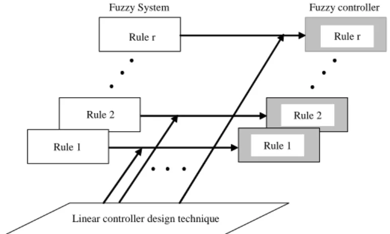
3.1 PDC controller design . . . 30

3.2 Angle response using two-rule fuzzy control for x1 = 30◦, 60◦, 85◦ and x2 = 0. . . 38

3.3 Angle response using two-rule fuzzy control for x1 = 85◦, 15◦, −85◦and x2 = 0. . . 39

3.4 Angle response using two-rule fuzzy control and m changed from 2.0 to 4.0 kg. . . 39

3.5 Angle response using two-rule fuzzy control and M changed from 8.0 to 4.0 kg. . . 40

3.6 Angle response using two-rule fuzzy control and 2l changed from 1.0 to 0.5 m. . . 40

4.1 Example 1 performances. . . 50

4.4 Example 4 (Two-link robot) performances: Link 1 (non-quadratic ap-proach) . . . 59

4.5 Example 4 (Two-link robot) performances: Link 2 (non-quadratic ap-proach) . . . 59

4.6 Example 4 (Two-links robot) performances: Link 1 (quadratic approach)

61

4.7 Example 4 (Two-links robot) performances: Link 2 (quadratic approach)

61

(8)

4.8 V (x (t)) with non-quadratic approach . . . .. 62

4.9 V (x (t)) with quadratic stabilization . . . .. 62

5.1 Inverted pendulum performances with a pole placement . . . 73

5.2 Inverted pendulum action evolution with a pole placement . . . 73

5.3 Inverted pendulum performances without pole placement . . . 75

5.4 Inverted pendulum action evolution without pole placement . . . 76

5.5 TORA performances . . . 79

(9)

Introduction

1.1 Context and motivations

During the last decade, fuzzy logic has attracted great attention, because of its ability to simultaneously handle numerical data and linguistic data knowledge. Fuzzy sets theory was first introduced in the landmark paper of Zadeh (Zadeh, 1965) at berekly university. Fuzzy logic is a powerful problem-solving methodology with a myriad of applications embedded in control and information processing since 70’s years, such as Mamdani which concretizes the first time this method to realize a fuzzy control in an industrial application (Mamdani, 1974),(Mamdani, 1977). Hence, unlike classical logic, which requires a deep understanding of a system, exact equations and precise numeric values, fuzzy logic incorporates an alternative way of thinking, which allows modeling complex systems using a higher level of abstraction originating from our knowledge and experience. The human expertise is used to construct a set of fuzzy rules of the form ”IF X is A THEN Y is B”, allowing the construction of fuzzy models, especially for systems that are diﬃcult to modelize, and consequently the number of applications based on fuzzy logic increased these last years considerably such as modelization, control, signal processing, pattern recognition and expert systems fields. The principal advantage of fuzzy logic systems is their aptitude to approximate any nonlinear function; they are universal approximators (Wang & Mendel, 1992). Many researches have been developed to demonstrate this concept (Kosko, 1994),(Castro, 1995),(Ying, 1998),(Zeng et al. , 2000),(Sala & Arino, 2007). The common point of this researches is the capability of a fuzzy model to approximate and then to represent any real function. A theoretical justification of fuzzy models as universal approximators has been given by wang (Wang & Mendel, 1992) for standard fuzzy systems with gaussian membership functions, product implication, conjunction and center of gravity defuzzification.

(10)

A fuzzy model is an expression of the system of interest in the framework of a fuzzy logic. There exist two kinds of fuzzy models: Mamdani fuzzy models and Takagi-Sugeno (T-S) fuzzy models. The advantage of T-S fuzzy models is their powerful capability to represent a complex nonlinear relationship in spite of a smaller number of fuzzy IF-THEN rules, than that of the Mamdani model. Moreover, in this type of model, the passage from one rule to another is done by a smooth transition from one rule to another, i.e., an interpolation between the rules.

In the literature, it appears that the most important application of fuzzy logic is fuzzy control, that was developed in Europe from the eighties and whose many researches works were produced such as in japan (Takagi & Sugeno, 1985), in the following decade. Takagi and Sugeno (Takagi & Sugeno, 1985) proposed a multimodel based approach to overcome the diﬃculties of the conventional modeling techniques. The proposed multimodel (T-S) is a convex polytopic form and can be obtained from identification approach (Sugeno & Kang, 1995),(Babuska, 1998) or from nonlinear dynamical model, by linearization, by the principle of sector nonlinearity (Kawamoto et al. , 1992) or by local approximation (Tanaka & Wang, 2001, a). For this purpose, a nonlinear plant is represented by the T-S fuzzy model, where local dynamics in diﬀerent state regions are represented by linear models. The overall model of the system is obtained by a fuzzy blending of these local models. This same fuzzy structure is used to control (Takagi & Sugeno, 1985),(Tanaka & Sugeno, 1992) (Wang et al. , 1996),(Feng, 2002) and to study the stability of the T-S fuzzy system using Lyapunov method (Tanaka & Sugeno, 1992),(Zhao, 1995) and Linear Matrix Inequalities (LMI), where the problem can be numerically solved by convex optimization techniques (Tanaka & Sugeno, 1992),(Boyd et al. , 1994),(Tanaka et al. , 2001, b).

The most used fuzzy control design in the literature is carried out using the Parallel Distributed Compensation (PDC) scheme (Tanaka & Sugeno, 1992),(Wang et al. , 1996) since it shares the same membership functions of the T-S fuzzy model. The main idea of the PDC controller design is to derive each linear control rule from the corresponding rule of T-S fuzzy model so as to compensate it. The resulting overall fuzzy controller, which is nonlinear in general, is a fuzzy blending of the local linear controllers, knowing that the fuzzy controller shares the same fuzzy sets with the fuzzy model. Wang et al. (Wang et al. , 1996) used this concept to design fuzzy controllers to stabilize T-S fuzzy systems.

The advantage of the T-S fuzzy model lies in that the stability and performance characteristics of the system represented by a T-S model can be analyzed using Lya-punov function approach (Tanaka & Sugeno, 1992),(Zhao, 1995). Tanaka and Sugeno (Tanaka & Sugeno, 1992) showed that the stability of a T-S fuzzy model could be shown by finding a common symmetric positive definite matrix P for r sub-models,

(11)

that satisfy a set of Lyapunov inequalities (Tanaka et al. , 1996),(Wang et al. , 1996). Hence, stability conditions are derived using a Lyapunov stability criteria for the fuzzy model , leading usually to Linear Matrix Inequalities (LMI) conditions, which are nu-merically tractable. Diﬀerent works have been realized based on this approach, such as Lee et al. (Lee et al. , 2001) who proposed a robust fuzzy control scheme for non-linear systems in the presence of parametric uncertainties, where suﬃcient conditions were derived for robust stabilization in the sense of Lyapunov stability and Cao and Lin (Cao & Lin, 2003) who applied the Lyapunov function based approach for the stability analysis of nonlinear systems with actuator saturation. On the other hand,

Tsen et al. (Tsen et al. , 2001) proposed a fuzzy H_∞ model reference tracking control

scheme and discussed the stability of the closed loop nonlinear system by Lyapunov approach, and Korba et al. (Korba et al. , 2003) presented a constructive and au-tomated method for the design of a gain-scheduling controller, based on a given T-S fuzzy model and a controller that guarantees the closed loop stability using Lyapunov quadratic functions. However, a possible limitation of their approaches is the use of the quadratic Lyapunov method, which is conservative. The quadratic approach re-quires to find a common positive definite matrix P for r sub-models, what makes it very conservative and hence brings us to search for less conservative stability condi-tions. Thus, having a T-S fuzzy model, the fundamental diﬃculty which arises during the synthesis of PDC controller is the conservatism of the stability conditions. By consequent, with an aim of having less conservative results , LMI relaxed conditions were the object of several works, in particular those developed in (Tanaka et al. , 1998) where the authors base themselves on the maximum number of active rules at each moment to reduce the conservatism of stabilization conditions. Kim and Lee (Kim & Lee, 2000) take as a starting point this work, by introducing additional conditions. In (Cao et al. , 1997),(Jadbabaie, 1999),(Chadli et al. , 2000),(Tanaka et al. , 2001, c),(Hadjili, 2002),(Teixeira et al. , 2003), the authors propose to use multiple Lya-punov functions to search for several positive definite matrices instead of searching for a common one, using quadratic Lyapunov function. Whereas, Johansson (Johansson et al. , 1999, a),(Rantzer & Johansson, 2000) used piecewise Lyapunov functions to reduce conservatism.

However, the states of a system are not always available for measurement which is the case in a lot of practical problems. To overcome this limit, the notion of observer was introduced. The concept of linear regulator and linear observer were introduced by Kalman (Kalman, 1961) for linear systems in stochastic environment and by Lu-enberger (LuLu-enberger, 1966) for deterministic linear systems, whereas for nonlinear systems, diﬀerent observer designs were proposed such as the extended kalman ob-server, the sliding mode observer (Utkin & Drakunov, 1995), the high gain observer

(12)

(Nicosia & Tornambe, 1989) and the T-S fuzzy observer, that was introduced by sev-eral authors in the literature such as Tanaka (Tanaka & Sano, 1994), Feng et al. (Feng et al. , 1997),(Lee et al. , 2001) who proposed fuzzy observers with an asymptotic convergence. Tanaka proposed in his paper (Tanaka et al. , 1998) a globally exponen-tially stable fuzzy controllers and fuzzy observers designs for continuous and discrete fuzzy systems for both measurable and non measurable premise variables. Other ap-proaches were proposed by diﬀerent authors, among them, Fayaz (Fayaz, 2000) who combined the results of (Tanaka et al. , 1998),(Fayaz, 1999) by using local Lyapunov functions to prove the existence of globally and quadratically stabilizing regulator and observer, Ma and Sun (Ma & Sun, 2001) for T-S fuzzy systems analysis and design of reduced-dimensional fuzzy observer and fuzzy functional observer with a separation property, and also (Cao & Frank, 2000),(Chen & Liu, 2004),(Wang, 2004),(Chen & Liu, 2005),(Lin et al. , 2006) and (Lin et al. , 2008) with other considerations. Hence, the observer design is a very important problem in control systems and the stability of the whole system, with the fuzzy controller and the fuzzy observer, must be guar-anteed. For a T-S fuzzy system, a separation property is used to check the stability of the global system. This concept was introduced by Jadbabaie et al. (Jadbabaie, 1997, b) and Ma et al. (Ma et al. , 1998) by diﬀerent approaches to assure an independent design for the controller and the observer while assuring the stability of the global T-S system.

1.2 Objectives and contributions

The objective of this research is the development of new Lyapunov stability condi-tions for continuous T-S fuzzy systems, in order to reduce the degree of conservatism. Hence, new non-quadratic stability conditions are derived based on PDC to stabilize continuous T-S fuzzy models. We use the fuzzy Lyapunov function since it is smooth contrary to the piecewise Lyapunov function thus avoiding the boundary condition problem. We obtain new conditions, shown to be less conservative, that stabilize con-tinuous fuzzy systems including those that do not admit a quadratic stabilization. Our approach is based on two assumptions. The first one relies on the existence of a proportionality relation between multiple quadratic Lyapunov functions, and the sec-ond one considers an upper bound for the time derivative of the premise membership function as assumed by Tanaka et al. (Tanaka et al. , 2001, b),(Tanaka et al. , 2001, c),(Tanaka et al. , 2001, d),(Tanaka et al. , 2003). We extend the stability results given in (Abdelmalek et al. , 2007) to the case of non available states for measurement and feedback, i.e. to the fuzzy observer conception, while guaranteeing the stability of the whole system. Whereas, we applied the separation principle of Ma et al.(Ma

(13)

et al. , 1998), due to its simplicity, since it does not depend on the stability conditions but rather on the fuzzy Lyapunov functions. Indeed, the separation principle design proposed in (Jadbabaie, 1997, b) is not appropriated for the case of several stability conditions. All these steps are illustrated by diﬀerent examples.

1.3 Organization of the thesis

This thesis is organized as follows:

Chapter 2 introduces the fuzzy modeling by two particular structures of fuzzy sys-tems that are Mamdani fuzzy syssys-tems and T-S fuzzy syssys-tems, followed by the diﬀerent construction methods of T-S fuzzy models due to their interesting characteristics. Dif-ferent existing methods for constructing a T-S fuzzy model are detailed and illustrated by diﬀerent examples. This chapter finishes by a theorem on the concept of "fuzzy systems are universal approximators", for any real continuous function.

Chapter 3 is devoted to quadratic stability and stabilization of T-S fuzzy systems by Lyapunov method. First, a recall is given on stability definition in the Lyapunov sense. Then quadratic stability conditions proposed by Tanaka (Tanaka & Sugeno, 1992),(Tanaka & Wang, 2001, a) are given for continuous T-S fuzzy systems. An out-line is given on an important tool in control theory, Linear Matrix Inequalities and some standards LMI problems. Also, a brief recall on the state of the art of existing fuzzy control laws such as parallel distributed compensation (PDC), compensation and division for fuzzy models (CDF), state feedback control and fuzzy simultaneous stability (FSS). This chapter finishes with quadratic stabilization of T-S fuzzy mod-els, especially, the continuous case which is considered in this thesis, starting by the example of the inverted pendulum given at the end of this chapter.

Chapter 4 is devoted to non-quadratic stability and stabilization of T-S fuzzy sys-tems by Lyapunov method. Due to the limitation of the quadratic approach by the conservatism constraint, new non-quadratic stability conditions are proposed (Abdel-malek et al. , 2007). The control design is based on PDC concept. The new conditions are shown to be less conservative and allow stabilization of continuous T-S fuzzy sys-tems including those that do not admit a quadratic stabilization.

Chapter 5 deals with the case of fuzzy control in presence of non measurable states. The fuzzy observer is designed separately from the fuzzy controller using the new non-quadratic stability conditions and applying a separation property to check the stability of the whole fuzzy system.

The thesis finishes with concluding remarks for this research and some prospects for the future.

(14)

• A non-quadratic fuzzy stabilization and tracking approach to a two link robot manipulator (Abdelmalek & Goléa, 2006).

• A new fuzzy Lyapunov approach to non-quadratic stabilization of Takagi-Sugeno fuzzy models (Abdelmalek et al. , 2007).

• Fuzzy observer design for Takagi-Sugeno fuzzy models via Linear Matrix Inequal-ities (Abdelmalek & Goléa, 2007, a).

• Model-based fuzzy control of an inverted pendulum on a cart: fuzzy controller and fuzzy observer design via LMIs (Abdelmalek & Goléa, 2008).

• LMI-based design of fuzzy controller and fuzzy observer for continuous Takagi-Sugeno fuzzy systems: new non-quadratic stability approach (Abdelmalek & Goléa, 2009).

(15)

Takagi-Sugeno Fuzzy Models

2.1 Introduction

Fuzzy sets theory and fuzzy logic provide the means for constructing fuzzy systems. Fuzzy sets were introduced by Professor L.A. Zadeh from berekley university in 1965 (Zadeh, 1965). Fuzzy logic provides a simple way to arrive at a definite conclusion based upon vague, ambiguous, imprecise, noisy, or missing input information. It is a powerful problem-solving methodology with a myriad of applications embedded in control and information processing since 70’s years, such as Mamdani that concretizes the first time this method to realize a fuzzy control in an industrial application (Mam-dani, 1974). Hence, unlike classical logic, that requires a deep understanding of a system, exact equations and precise numeric values, fuzzy logic incorporates an alter-native way of thinking, which allows modeling complex systems using a higher level of abstraction originating from our knowledge and experience. The principal advantage of fuzzy logic systems is their aptitude to approximate any nonlinear function; they are universal approximators (Wang & Mendel, 1992). Takagi and Sugeno (Takagi & Sugeno, 1985) came up with an alternative rule format in order to make automated tuning possible and to reduce the number of fuzzy rules needed to construct the fuzzy model. Two particular structures of fuzzy systems will be detailed, followed by the advantages and the disadvantages of the one compared to the other.

In this chapter, a recall is given on modeling by two particular structures of

fuzzy models that are Mamdani and T-S fuzzy models, followed by the advantages and the disadvantages of the one compared to the other. however, the construction procedure of a T-S fuzzy model is detailed. An outline is given on the concept of universal approximators, to show that a fuzzy model is able to approximate and then to represent any real function.

(16)

Numerical output ℜ ∈ V Numerical input Defuzzifier Fuzzifier

Output fuzzy sets in V

Input fuzzy sets in U Fuzzy model ℜ ∈ U Rules Inference

Figure 2.1: Fuzzy model structure

2.2 Fuzzy modeling

Fuzzy modeling is to construct a model through a description language based on fuzzy logic. It gives a qualitative description of systems functions and behaviors using a natural language. A fuzzy model consists, in general of four basic components: a fuzzy rule base, a fuzzy inference engine, a fuzzifier and a deﬀuzifier as shown in figure (2.1) (Wang, 1994),(Mendel, 1995),(Zhao, 1995).

• Fuzzy rule base is the knowledge base of the system to be modeled. It is a collection of IF-THEN rules, in general of the following form

Model Rule i : IF z1(t) is Mi1and ... and zp(t) is Mip THEN y is Bi (2.1)

where z = [z1, z2, ..., zp]T ∈ Rpis the input, y is the output and both are linguistic

variables in the input product space U1× U2× ... × Up and in the output space

V. Mi1, Mi2, ..., Mip and Bi are fuzzy sets. i ∈ [1, r] , r is the number of rules in

the fuzzy rule base.

• Fuzzy inference engine is a rule-based system that uses fuzzy logic, rather than Boolean logic, to reason about data. It simulates the human decision-making process by using fuzzy logic, and its task is to interpret and to construct an input-output mapping relationship with respect to all the rules.

• Fuzzifier performs the conversion from numerical values of input variables

z1, z2, ..., zp, obtained by sensors, into linguistic values represented as fuzzy sets

(17)

• Defuzzifier performs the inverse conversion of that performed by the fuzzifier, i.e. conversion from the linguistic values in the form of fuzzy sets into non-fuzzy crisp values. Three kind of defuzzifier are employed in general: maximum defuzzifier, center average defuzzifier, and modified center average defuzzifier (Wang, 1994).

However, there exist two kinds of fuzzy models: Mamdani fuzzy models and T-S fuzzy models.

2.2.1 Mamdani fuzzy models

In this kind of fuzzy models, the fuzzy IF-THEN rules are of the following form:

Rule i : IF z1(t) is Mi1and ... and zp(t) is Mip THEN y is Bi (2.2)

The main advantages of this type of model are:

• the simplicity in representation of fuzzy rules,

• the flexibility in implementation ; due to the freedom to choose the operations

included in fuzzy models.

The main disadvantage of this model is the great number of rules needed to repre-sent a complex nonlinear system.

2.2.2 T-S fuzzy models

Takagi and Sugeno (Takagi & Sugeno, 1985) came up with the alternative rule format (2.3) in order to make automated tuning possible and to reduce the number of fuzzy rules. A T-S fuzzy model is described by fuzzy IF-THEN rules defined by the following

Rule i : IF z1(t) is Mi1 and ... and zp(t) is Mip

THEN yi = ai₀+ ai₁z1(t) + ai2z2(t) + ... + aipzp(t) (2.3)

where Mi1, ..., Mip are fuzzy sets; ai0, ..., aip are the coeﬃcients of the i-th linear

con-sequent and is the output of the i-th fuzzy IF-THEN rule. The crisp output value of

the T-S fuzzy model is a weighted average of the yi is:

y = Pr i=1wi(t) yi Pr i=1wi(t) (2.4)

where 0 ≤ wi(t) ≤ 1, Pri=1wi(t) > 0 and wi(t) = Πpj=1 Mij(zj(t)) , Mij(zj(t))

is the grade of membership of zj(t) in Mij. The equation (2.3) gives an aﬃne

T-S fuzzy model, for ai₀ = 0, we have a linear T-S model. T-S model represents a

dynamical system whose IF-THEN rules represent local linear input-output relations of the nonlinear dynamical system. The main feature of a T-S fuzzy model is to express

(18)

the local dynamics of each fuzzy rule by a linear sub-model, and then the overall fuzzy system is obtained by fuzzy “blending” of the linear sub-models (Tanaka & Wang, 2001, a).

The advantage of T-S fuzzy models is their powerful capability to represent a complex nonlinear relationship in spite of the smaller number of fuzzy IF-THEN rules, than that of Mamdani fuzzy models. These latter, with a centroid deﬀuzification, can be seen as a particular case of T-S fuzzy models. Moreover, in a T-S fuzzy model, the passage from one rule to another is done by a smooth transition between the rules, i.e., an interpolation. Thus (2.4) interpolates between diﬀerent linear functions, that are the local models (figure (2.2)).

y

( )

x A

μ

3

( )

x

A

μ

1

( )

x A

μ

2

( )

x

f

1

_f

( )

_x

3

( )

x

f

₂

x

Figure 2.2: A function f defined by a T-S model

2.3 Construction of a T-S fuzzy model

In general, there exist two ways to construct a fuzzy model: by identification us-ing input-output data (in other terms fuzzy modelus-ing) or by derivation from a given nonlinear system equations.

(19)

Nonlinear system

Identification using

input-output data Physical model

Fuzzy model (Takagi-Sugeno fuzzy model)

Fuzzy controller

Parallel distributed compenstion (PDC)

Figure 2.3: Model-based fuzzy control design

The identification approach is suitable for the modelization of plants that are dif-ficult to represent using analytical models, whereas when the nonlinear dynamical models are available, the second approach is more appropriated (Tanaka & Wang, 2001, a). In both cases, we obtain a T-S fuzzy model whose ith rule form is:

Rule i : IF z1(t) is Mi1 and ... and zp(t) isMip

THEN

( _.

x (t) = Aix (t) + Biu (t) y (t) = Cix (t)

i = 1, 2, ..., r (2.5)

The final outputs of the fuzzy model are inferred as follows:

( _.

x (t) =Pr_i=1hi(z (t)) (Aix (t) + Biu (t)) y (t) =Pr_i=1hi(z (t)) Cix (t)

(2.6)

where z (t) = [z1(t) , ..., zp(t)] is the premise variable vector that may be functions

of the state variables, measurable external disturbances and/or time. Ai ∈ <n×n,

Bi ∈ <n×m, Ci ∈ <q×n, x (t) ∈ <n is the state vector, u (t) ∈ <m is the input vector,

y (t) ∈ <q is the output vector. r is the number of IF-THEN rules and Mij is a fuzzy

set. hi(z (t)) is the normalized weight for each rule, that is

hi(z (t)) ≥ 0, r X

i=1

(20)

and is given by: hi(z (t)) = wi(t) Pr i=1wi(t)

2.3.1 Identification approach

From input-output data, we obtain linear sub-models around the diﬀerent operational points. The local linear sub-models, are fuzzy IF-THEN rules, whose consequent parts are linear models. This identification allows us to find an optimal model after estimat-ing the parameters and validatestimat-ing, the final model (Sugeno & Kang, 1995),(Babuska, 1998). However, a state representation is used in the consequent part in order to extend the state feedback control principle to the nonlinear case.

2.3.2 Nonlinear dynamical model

When nonlinear dynamical models are easy to obtain, the linearization, the principle of sector nonlinearity or local approximation are more appropriated for constructing the fuzzy model (Tanaka & Wang, 2001, a).

Linearization

The basic idea is to linearize the nonlinear analytical model of the process about diﬀerent operating points. Hence for the following nonlinear system

.

x (t) = f (x (t) , u (t)) ; f (·) ∈ C1 (2.7)

The linearization of the system around an arbitrary operating point (xi, ui) ∈ Rn×Rp,

we have then: .

x (t) = Ai(x (t) − xi) + Bi(u (t) − ui) + f (xi, ui) (2.8)

Taking wi = f (xi, ui) − Aixi− Biui, equation (2.8) can be rewritten:

.

x (t) = Aix (t) + Biu (t) + wi (2.9)

where Ai = ∂f (x,u)_∂x |x=xi

u=ui

and Bi = ∂f (x,u)_∂u |x=xi

u=ui

By considering that the local sub-models result from the linearization about r operational points, the T-S Fuzzy model is given by:

. x (t) = r X i=1 hi(z (t)) (Aix (t) − Biu (t) + wi) (2.10)

(21)

Sector nonlinearity

The first apparition of sector non linearity in fuzzy model construction was in 1992 by Kawamoto et al. (Kawamoto et al. , 1992), it is based on considering a simple

nonlinear system x (t) = f (x (t)) where f (0) = 0. The objective is to find the global.

sector such that_{x (t) = f (x (t)) ∈}. h _{−a a} ix (t) , as illustrated in figure 2.4. An exact

fuzzy model construction is guaranteed with this method. However, it is sometimes diﬃcult to find global sectors, then local sector nonlinearity is considered, where x (t) ∈ h

−d d i

. Figure 2.5 shows the local sector nonlinearity, where two lines become the local sectors under −d < x (t) < d. The nonlinear system is represented exactly by the fuzzy model in the “local” region −d < x (t) < d. But, it is often desirable to simplify the original nonlinear system as much as possible in order to reduce the number of rules. the following two examples illustrates this concept.

( )t x ( )t x a2 ( )t x a1 ( ) ( )xt f

(22)

( )t x ( ) ( )xt f d − d

Figure 2.5: Local sector nonlinearity Example 1

For the following nonlinear system (Tanaka & Wang, 2001, a): " . x1 . x2 # = " −x1(t) + x1(t) x32(t) −x2(t) + (3 + x2(t)) x31(t) # x (t) (2.11)

it is assumed for simplicity that x1(t) ∈

h −1 1 i and x2(t) ∈ h −1 1 i , then (2.11) can be written as . x (t) = " −1 x1(t) x22(t) (3 + x2(t)) x21(t) −1 # x (t) where x (t) =h x1(t) x2(t) iT

and x1(t) x22(t) and (3 + x2(t)) x21(t) are nonlinear terms. By defining z1(t) ≡ x1(t) x22(t) and z2(t) ≡ (3 + x2(t)) x21(t) we have: . x (t) = " −1 z1(t) z2(t) −1 # x (t) .

Then, the minimum and maximum values are calculated under x1(t) ∈

h −1 1 i and x2(t) ∈ h −1 1 i

, their values are: max x1(t),x2(t) z1(t) = 1, min x1(t),x2(t) z1(t) = −1 max x1(t),x2(t) z2(t) = 4, min x1(t),x2(t) z2(t) = 0

(23)

From these values, z1(t) and z2(t) can be represented by: z1(t) ≡ x1(t) x22(t) = M1(z1(t)) · 1 + M2(z1(t)) · (−1) z2(t) ≡ (3 + x2(t)) x21(t) = N1(z2(t)) · 4 + N2(z2(t)) · 0 where M1(z1(t)) + M2(z1(t)) = 1 N1(z2(t)) + N2(z2(t)) = 1 Therefore the membership functions can be calculated by:

M1(z1(t)) = z1(t) + 1 2 , M2(z1(t)) = 1 − z1(t) 2 N1(z2(t)) = z2(t) 4 , N2(z2(t)) = 4 − z2(t) 4

These membership functions are named respectively: "Positive", "Negative", "Big" and "Small". Hence, equation (2.11) can be represented by the following fuzzy model:

Rule 1 : IF z1(t) is ”P ositive” and z2(t) is ”Big” THEN

.

x (t) = A1x (t)

Rule 2 : IF z1(t) is ”P ositive” and z2(t) is ”Small” THEN

.

x (t) = A2x (t)

Rule 3 : IF z1(t) is ”N egative” and z2(t) is ”Big” THEN

.

x (t) = A3x (t)

Rule 4 : IF z1(t) is ”N egative” and z2(t) is ”Small” THEN

. x (t) = A4x (t) where A1 = " −1 1 4 ₋₁ # , A2 = " −1 1 0 ₋₁ # A3 = " −1 −1 4 ₋₁ # , A4 = " −1 −1 0 ₋₁ #

The deﬀuzification yields: . x (t) = 4 X i=1 hi(z (t)) Aix (t) where h1(z (t)) = M1(z1(t)) × N1(z2(t)) h2(z (t)) = M1(z1(t)) × N2(z2(t)) h3(z (t)) = M2(z1(t)) × N1(z2(t)) h4(z (t)) = M2(z1(t)) × N2(z2(t))

Finally, this model represents the nonlinear system in the regionh _{−1 1} i_×h _{−1 1} i

(24)

Example 2

For the inverted pendulum defined by the following equations of motion (Tanaka & Wang, 2001, a):

.

x1(t) = x2(t) ,

.

x2(t) =

g sin (x1(t)) − amlx22(t) sin (2 (x1(t))) /2 − a cos (x1(t)) u (t)

4l/3 − aml cos2_(x

1(t))

(2.12)

where x1(t) denotes the angle (in radians) of the pendulum from the vertical and

x2(t) is the angular velocity, g = 9.8 m/s2 is the gravity constant, m is the mass

of the pendulum. M is the mass of the cart, 2l is the length of the pendulum, u is the force applied to the cart (in newtons) and a = 1/ (m + M ). Equation (2.12) is rewritten as . x2(t) = gx1(t) − au (t) 4l/3 − aml × µ g sin (x1(t)) − amlx2(t) sin (2x1(t)) 2 x2(t) − a cos (x1(t)) u (t) ¶ (2.13) Define z1(t) ≡ 1 4l/3 − aml cos2_(x 1(t)) z2(t) ≡ sin (x1(t)) z3(t) ≡ x2(t) sin (2x1(t)) z4(t) ≡ cos (x1(t)) where x1(t) ∈ (−π/2, π/2) and x2(t) ∈ h −α α i

. To maintain controllability of the

fuzzy model, we assume that x1(t) ∈ [−88◦, 88◦] . Equation (2.13) is rewritten as

. x2(t) = z1(t) ½ gz2(t) − aml 2 z3(t) x2(t) − az4(t) u (t) ¾

we replace z1(t) − z4(t) with T-S fuzzy model representation. Since

max z1(t) = 1 4l/3 − amlβ2 ≡ q1, β = cos (88 ◦_{) ,} min z1(t) = 1 4l/3 − aml ≡ q2, z1(t) can be rewritten as z1(t) = 2 X i=1 Ei(z1(t)) qi (2.14)

(25)

where E1(z1(t)) = z1(t) − q2 q1− q2 , E2(z1(t)) = q1− z1(t) q1− q2

These membership functions are obtained from the property of E1(z1(t))+E2(z1(t)) =

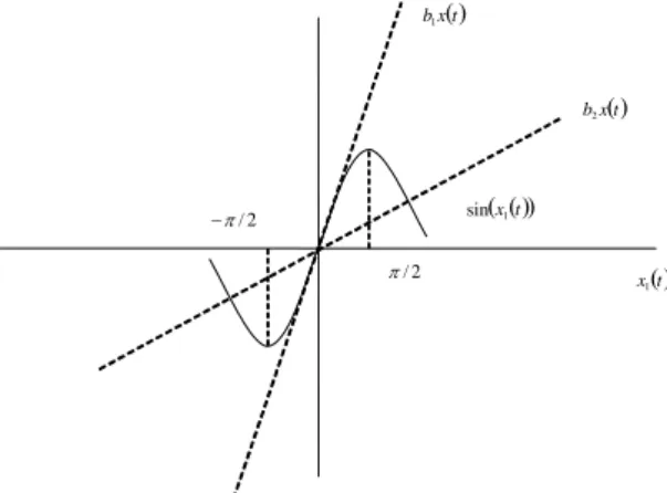
1. Figure 2.6 shows the local sector of z2(t) = sin (x1(t)) for x1(t) ∈ (−π/2, π/2) .

The sector [b1, b2] consists of two lines b1x1 and b2x1, where b1 = 1 and b2 = 2/π are

the slopes ( )t x1 ( ) (x1t) sin 2 / π − 2 / π ( )t x b1 ( )t x b2

Figure 2.6: sin (x1(t)) and its sector

Therefore sin (x1(t)) is represented as follows:

z2(t) = sin (x1(t)) = Ã ₂ X i=1 Mi(z2(t)) bi ! x1(t) (2.15)

Then, from [M1(z2(t)) + M2(z2(t)) = 1] , the membership functions are

M1(z2(t)) = ½z2(t)−(2/π) sin−1(z2(t)) (1−2/π) sin−1(z2(t)) , z2(t) 6= 0 1, otherwise M2(z2(t)) = ½(2/π) sin−1_(z₂_(t))−z₂_(t) (1−2/π) sin−1_(z₂_(t)) , z2(t) 6= 0 0, otherwise

We consider next, z3(t) = x2(t) sin (2x1(t)) . Since

max x1(t),x2(t)

z3(t) = α ≡ c1 and min

x1(t),x2(t)

z3(t) = −α ≡ c2

In the same way as for the z1(t) case:

z3(t) = x2(t) sin (2x1(t)) = 2 X

i=1

(26)

where N1(z3(t)) = z3(t) − c2 c1− c2 , N2(z3(t)) = c1− z3(t) c1− c2

The same procedure is applied for z4(t) . Since

max x1(t) z4(t) = 1 ≡ d1 and min x1(t) z4(t) = β ≡ d2 we obtain z4(t) = cos (x1(t)) = 2 X i=1 Si(z4(t)) di (2.17) where S1(z4(t)) = z4(t) − d2 d1− d2 , S2(z4(t)) = d1− z4(t) d1− d2

From (2.14)-(2.17), the following T-S fuzzy model is constructed for the inverted pen-dulum: ∙. x1(t) . x2(t) ¸ = 2 X i=1 2 X j=1 2 X k=1 2 X l=1 Ei(z1(t)) Mj(z2(t)) Nk(z3(t)) Sl(z4(t)) × Ã" 0 1 gqibj −aml₂ qick # ∙ x1(t) x2(t) ¸ + " 0 −aqidl #! = 2 X i=1 2 X j=1 2 X k=1 2 X l=1 Ei(z1(t)) Mj(z2(t)) Nk(z3(t)) Sl(z4(t)) × {Aijklx (t) + Bijklu (t)} (2.18)

The summations in (2.18) can be aggregated as one summation: . x (t) = 16 X ρ=1 hρ(z (t)) © A∗_ρx (t) + B_ρ∗u (t)ª (2.19) where ρ = l + 2 (k − 1) + 4 (j − 1) + 8 (i − 1) , hρ(z (t)) = Ei(z1(t)) Mj(z2(t)) Nk(z3(t)) Sl(z4(t)) , A∗_ρ= Aijkl, Bρ∗ = Bijkl

Equation (2.19) means that the fuzzy model has the following 16 rules:

Rule 1: ⎧ ⎪ ⎨ ⎪ ⎩

IF z1(t) is ”P ositive” and z2(t) is ”Zero”

and z3(t) is ”P ositive” and z4(t) is ”Big”

THENx (t) = A. ∗

(27)

Rule 2: ⎧ ⎪ ⎨ ⎪ ⎩

and z3(t) is ”P ositive” and z4(t) is ”Small”

THENx (t) = A. ∗₂x (t) + B₂∗u (t) Rule 3: ⎧ ⎪ ⎨ ⎪ ⎩

and z3(t) is ”N egative” and z4(t) is ”Big”

THENx (t) = A. ∗₃x (t) + B₃∗u (t) Rule 4: ⎧ ⎪ ⎨ ⎪ ⎩

and z3(t) is ”N egative” and z4(t) is ”Small”

THENx (t) = A. ∗₄x (t) + B₄∗u (t) Rule 5: ⎧ ⎪ ⎨ ⎪ ⎩

IF z1(t) is ”P ositive” and z2(t) is ”N ot Zero”

THENx (t) = A. ∗₅x (t) + B₅∗u (t) Rule 6: ⎧ ⎪ ⎨ ⎪ ⎩

THENx (t) = A. ∗₆x (t) + B₆∗u (t) Rule 7: ⎧ ⎪ ⎨ ⎪ ⎩

THENx (t) = A. ∗₇x (t) + B₇∗u (t) Rule 8: ⎧ ⎪ ⎨ ⎪ ⎩

THENx (t) = A. ∗₈x (t) + B₈∗u (t) Rule 9: ⎧ ⎪ ⎨ ⎪ ⎩

IF z1(t) is ”N egative” and z2(t) is ”Zero”

THENx (t) = A. ∗₉x (t) + B₉∗u (t) Rule 10: ⎧ ⎪ ⎨ ⎪ ⎩

THENx (t) = A. ∗₁₀x (t) + B∗₁₀u (t) Rule 11: ⎧ ⎪ ⎨ ⎪ ⎩

THENx (t) = A. ∗₁₁x (t) + B∗₁₁u (t) Rule 12: ⎧ ⎪ ⎨ ⎪ ⎩

(28)

Rule 13: ⎧ ⎪ ⎨ ⎪ ⎩

IF z1(t) is ”N egative” and z2(t) is ”N ot Zero”

THENx (t) = A. ∗₁₃x (t) + B₁₃∗ u (t) Rule 14: ⎧ ⎪ ⎨ ⎪ ⎩

THENx (t) = A. ∗₁₄x (t) + B₁₄∗ u (t) Rule 15: ⎧ ⎪ ⎨ ⎪ ⎩

THENx (t) = A. ∗₁₅x (t) + B₁₅∗ u (t) Rule 16: ⎧ ⎪ ⎨ ⎪ ⎩

THENx (t) = A. ∗₁₆x (t) + B₁₆∗ u (t)

where z1(t) , z2(t) , z3(t) and z4(t) are premise variables and

A∗₁ = A1111 = " 0 1 gq1b1 −aml₂ q1c1 # , B₁∗= B1111 = " 0 −aq1d1 # , A∗₂ = A1112 = " 0 1 gq1b1 −aml₂ q1c1 # , B₂∗= B1112 = " 0 −aq1d2 # , A∗₃ = A1121 = " 0 1 gq1b1 −aml₂ q1c2 # , B₃∗= B1121 = " 0 −aq1d1 # , A∗₄ = A1122 = " 0 1 gq1b1 −aml₂ q1c2 # , B₄∗= B1122 = " 0 −aq1d2 # , A∗₅ = A1211 = " 0 1 gq1b2 −aml₂ q1c1 # , B₅∗= B1211 = " 0 −aq1d1 # , A∗₆ = A1212 = " 0 1 gq1b2 −aml₂ q1c1 # , B₆∗= B1212 = " 0 −aq1d2 # , A∗₇ = A1221 = " 0 1 gq1b2 −aml₂ q1c2 # , B₇∗= B1221 = " 0 −aq1d1 # , A∗₈ = A1222 = " 0 1 gq1b2 −aml₂ q1c2 # , B₈∗= B1222 = " 0 −aq1d2 # , A∗₉ = A2111 = " 0 1 gq2b1 −aml₂ q2c1 # , B₉∗= B2111 = " 0 −aq2d1 # ,

(29)

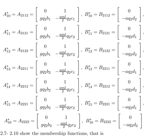
A∗₁₀= A2112= " 0 1 gq2b1 −aml₂ q2c1 # , B₁₀∗ = B2112= " 0 −aq2d2 # , A∗₁₁= A2121= " 0 1 gq2b1 −aml₂ q2c2 # , B₁₁∗ = B2121= " 0 −aq2d1 # , A∗₁₂= A2122= " 0 1 gq2b1 −aml₂ q2c2 # , B₁₂∗ = B2122= " 0 −aq2d2 # , A∗₁₃= A2211= " 0 1 gq2b2 −aml₂ q2c1 # , B₁₃∗ = B2211= " 0 −aq2d1 # , A∗₁₄= A2212= " 0 1 gq2b2 −aml₂ q2c1 # , B₁₄∗ = B2212= " 0 −aq2d2 # , A∗₁₅= A2221= " 0 1 gq2b2 −aml₂ q2c2 # , B₁₅∗ = B2221= " 0 −aq2d1 # , A∗₁₆= A2222 = " 0 1 gq2b2 −aml₂ q2c2 # , B₁₆∗ = B2222 = " 0 −aq2d2 #

Figures 2.7- 2.10 show the membership functions, that is E1(z1(t)) = z1(t) − q2 q1− q2 , E2(z1(t)) = q1− z1(t) q1− q2 M1(z2(t)) = sin (x1(t)) − (2/π) z2(t) (1 − 2/π) z2(t) , M2(z2(t)) = x1(t) − z2(t) (1 − 2/π) z2(t) N1(z3(t)) = z3(t) − c2 c1− c2 , N2(z3(t)) = c1− z3(t) c1− c2 S1(z4(t)) = z4(t) − d2 d1− d2 , S2(z4(t)) = d1− z4(t) d1− d2 Positive Negative ( ) (z t) E₁ ₁ ( ) (z t) E₂ ₁ 0 1 ( )t z1 aml l/3− 4 1 2 3 / 4 1 β aml l −

(30)

Zero Not zero

( )

(

z t

)

M₁ ₂

( )

(

z t

)

M₂ ₂ 0 1

( )

t z2 1 − 0 1

Figure 2.8: Membership functions M1(z2(t)) and M2(z2(t))

Positive Negative ( ) (z t) N₁ ₃ ( ) (z t) N₂ ₃ 0 1 ( )t z₃ α − 0 α

Figure 2.9: Membership functions N1(z3(t)) and N2(z3(t))

Big Small ( ) (z t) S1 4 ( ) (z t) S₂ ₄ 0 1 ( )t z₄ β 1 2 1+β

(31)

Local approximation in fuzzy partition spaces

The principle of this method is to approximate nonlinear terms by adequate chosen linear terms, that leads to a less number of rules. For example, Tanaka (Tanaka & Wang, 2001, a) proposed in his book a fuzzy modelization of an inverted pendulum with 16 rules using the sector nonlinearity method, whereas, using the local approximation, the inverted pendulum is represented by a two rules fuzzy model.

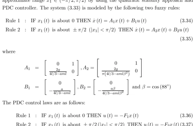
Example 3

For the inverted pendulum defined by equations of motion (2.12), the simplification leads to two cases:

when x1(t) is near zero we have:

. x1(t) = x2(t) , (2.20) . x2(t) = gx1(t) − au (t) 4l/3 − aml (2.21)

whereas when x1(t) is near ±π/2 we have:

. x1(t) = x2(t) , (2.22) . x2(t) = 2gx1(t) /π − aβu (t) 4l/3 − amlβ2 (2.23)

where β = cos (88◦) .The equations (2.20)-(2.23) are linear systems that produces the

following fuzzy modelization of the inverted pendulum:

Model Rule 1 : IF x1(t) is about 0 THEN

.

x (t) = A1x (t) + B1u (t)

Model Rule 2 : IF x1(t) is about ±π/2 (|x1| < π/2) THEN

.

x (t) = A2x (t)+B2u (t)

where the membership functions are of triangular types

Rule 1 Rule 2 0 1 -90 0 90 (deg) 1 x

(32)

and A1 = " 0 1 2g 4l/3−aml 0 # , A2= ⎡ ⎣ 2g0 1 π(4l/3−amlβ2₎ 0 ⎤ ⎦ B1= " 0 −_4l/3−amla # , B2 = " 0 −_4l/3−amlβaβ 2 # , β = cos (88◦)

2.4 Fuzzy systems as universal approximators

A fuzzy system can be regarded as a (multidimensional) input-output mapping y = f (x). Several authors have proved that given enough rules, the fuzzy system can ap-proximate any real continuous function to any given accuracy. The following theorem shows that the fuzzy logic system

f (x) = Pr l=1y¯l ∙ Πn_i=1al_iexp µ −³xi−¯xli σl i ´2¶¸ Pr l=1 ∙ Πn_i=1al_iexp µ −³xi−¯xli σl i ´2¶¸ (2.24)

with center average defuzzifier, product inference rule, singleton fuzzifier and gaussian membership function, is able to uniformly approximate any nonlinear function over U to any degree of accuracy.

Theorem 1 Universal approximation theorem (Wang & Mendel, 1992): For any

given real continuous function g on a compact set U ⊂ Rn and arbitrary > 0, there

exists a fuzzy logic system f in the form of (2.24) such that sup

x∈U|f (x) − g (x)| <

(2.25) This theorem provides a justification for applying the fuzzy logic systems to almost any nonlinear modeling problems.

2.5 conclusion

This chapter has recalled in first the two types of fuzzy models representations for complex systems, that are Mamdani fuzzy models and T-S fuzzy models. An atten-tion is given to T-S fuzzy models due to their interesting characteristics. Diﬀerent existing methods for constructing a T-S fuzzy model are detailed and illustrated by diﬀerent examples. This chapter finishes by a theorem on the concept of universal approximators of T-S fuzzy models.

(33)

Quadratic stability and

Stabilization of T-S Fuzzy

Systems

3.1 Introduction

This chapter deals with the fuzzy stability and stabilization of T-S fuzzy systems. During the last decade, several researchers in the control community have come up with different techniques for designing control systems. Fuzzy control is probably one of the most popular (Takagi & Sugeno, 1985),(Tanaka & Sugeno, 1992),(Wang et al. , 1996),(Feng, 2002), since it can provide an effective solution to the control of plants that are complex, uncertain or ill-defined, by combining the flexibility of fuzzy logic theory and the rigorous mathematical analysis tools in linear system theory into a unified framework. Tanaka and Sugeno (Tanaka & Sugeno, 1992) showed that finding common symmetric positive definite matrix P for N sub-systems could show the stability of continuous T-S fuzzy system. Generally, most of the stability criteria for this fuzzy system derived by Lyapunov approach needs a common P to satisfy a set of Lyapunov inequalities (Tanaka et al. , 1996),(Wang et al. , 1996). These inequalities can be reduced to LMI problems, that can be solved efficiently in practice by convex programming techniques for LMIs. The fuzzy controller is based on the PDC design with the principle of deriving each control rule from the corresponding rule of T-S fuzzy model so as to compensate it.

This chapter considers the stability and stabilization analysis of continuous T-S fuzzy models using Lyapunov approach, PDC and LMIs. LMIs are detailed in this chapter with some standard LMI problems used in control applications and an outline on the diﬀerent existing fuzzy control laws is given. Finally, the inverted pendulum

(34)

example illustrates these diﬀerent concepts.

3.2 Systems stability

The stability of systems in closed loop is one of the most significant problems in control theory. The T-S systems stability analysis was the objective of several works (Tanaka & Sugeno, 1992),(Wang et al. , 1996),(Jadbabaie, 1997, b),(Tanaka et al. , 1998),(Kim & Lee, 2000),(Manamanni et al. , 2007) by quadratic Lyapunov functions (Johansson et al. , 1999, a),(Rantzer & Johansson, 2000),(Chadli et al. , 2003),(Ohtake et al. , 2003),(Feng, 2004) by piecewise quadratic Lyapunov functions and (Blanco et al. , 2001),(Tanaka et al. , 2001, c),(Chadli et al. , 2002),(Tanaka et al. , 2003),(Teixeira et al. , 2003),(Guerra & Vermeiren, 2004),(Bernal & Hu˘sek, 2005),(Zhou et al. , 2007) by non-quadratic Lyapunov functions. In the majority, the goal was the obtention of a global asymptotic stability by applying Lyapunov’s direct method based on Lyapunov functions, which measure the system’s energy. Stability in the Lyapunov sense is a mathematical translation of an elementary observation: if the total energy of a system dissipates in a continuous manner (i.e. decreases with time), then this system (that it is linear or not, stationary or not) tends to an equilibrium state (it is stable). The direct method thus seeks to generate a scalar function of energy type which admits a negative temporal derivative. There exist some definitions related to Lyapunov stability, among them the following.

Definition 2 The equilibrium point xe is stable if

∀t ≥ 0, ∀ > 0, ∃α > 0 such that kx (0) − xek < α ⇒ kx (t) − xek <

in the contrary case xe is unstable.

In other terms, a system is stable in Lyapunov sense if and only if a weak distur-bance of the initial conditions involves a weak disturdistur-bance of the system trajectory. Another important definition in system control theory is the global asymptotic stabil-ity.

Definition 3 The equilibrium point xe = 0 is locally asymptotically stable if it is

stable and there exist r > 0 such that:

if kx (0)k < r then limt→∞kx (t)k → 0

Definition 4 if a system is asymptotically stable for any initial condition in Rn, then

(35)

3.3 Lyapunov functions in the control literature

In general, there is no a systematic method to find candidate Lyapunov functions. The degree of conservatism of the obtained stability conditions depends on the Lya-punov function form and the system structure. Diﬀerent LyaLya-punov functions forms are used by diﬀerent authors in the literature (Tanaka & Sano, 1994),(Wang et al. , 1996),(Tanaka et al. , 1998),(Wong et al. , 1998),(Jadbabaie, 1999),(Johansson et al. , 1999, a),(Chadli et al. , 2000),(Blanco et al. , 2001),(Chadli et al. , 2001),(Ohtake et al. , 2003),(Tanaka et al. , 2003),(Bernal & Hu˘sek, 2005), depending of the system nature and complexity.

3.3.1 Quadratic Lyapunov function

This one is the classical form, it is given by:

V (x (t)) = xT(t) P x (t) , P > 0, PT = P (3.1)

used initially to stability study of linear systems and then for MIMO nonlinear systems, in particular, T-S fuzzy systems (Tanaka & Sugeno, 1992),(Zhao, 1995),(Wang et al. , 1996),(Tanaka et al. , 1998). The principle of the method is to search a positive definite matrix P, by the way of convex formulation of the problem. The drawback of this quadratic approach is the conservative stability conditions, but it remains from a practical point of view easy to implement.

3.3.2 Non-quadratic Lyapunov function

This function is of the form: V (x (t)) =

r X i=1

hi(z (t)) xT(t) Pix (t) (3.2)

where Piis a positive definite matrix and hi(z (t)) ≥ 0,Pr_i=1hi(z (t)) = 1. It is a more

general function since it includes the quadratic case when Pi= P , i = 1, .., r. However,

an interesting advantage is that, the non-quadratic form of Lyapunov function takes into account the speed variation of the decision variables, what allows the conservatism reduction and more relaxed stability conditions. Indeed, it has been studied by many authors, (Jadbabaie, 1999),(Chadli et al. , 2000),(Morère, 2001),(Tanaka et al. , 2001, d), who concluded on the need to have an upper bounds on the speed variations of decision variables and then on the first time derivative of premise membership functions to reduce conservatism. On another side, this type of functions reduces the global stability of the nonlinear system to the analysis of the local stability of each local

(36)

linear model (sub-model) separately. However, this Lyapunov function was also used in the discrete case by several authors such as (Daafouz & Bernussou, 2001),(Morère, 2001).

3.3.3 Piecewise quadratic Lyapunov function

T-S fuzzy systems and aﬃne T-S fuzzy systems can be considered as piecewise linear systems. Hence, many authors such as (Johansson, 1999),(Johansson et al. , 1999, a),(Feng, 2002),(Ohtake et al. , 2003) proposed piecewise quadratic Lyapunov functions to reduce conservatism and whose search is based on a convex optimization problem, they are given by:

V (x) = ⎧ ⎪ ⎪ ⎨ ⎪ ⎪ ⎩ xTPix, , x ∈ Xi, i ∈ I0 " x 1 #T Pi " x 1 # , x ∈ Xi, i ∈ I1 (3.3)

where the operating region Xi is a partition in the state space and corresponds to a

dynamic local model i. Thus, the principle of the approach is to divide the space into two regions: an operating region and an interpolation region. This Lyapunov function combines the power of quadratic Lyapunov functions near an equilibrium point with the flexibility of piecewise linear functions in the large. It also allows conservatism reduction because of the space partionning induced by a locally bounded membership

function. This leads to search for a common Pi to all active local linear models in

each region. However, the conservatism reappears for this approach when the number of activated local models becomes equal to the total number of local models.

3.4 Quadratic stability of Takagi-Sugeno fuzzy systems

In this section quadratic Lyapunov functions are considered whose one of the existing definitions is:

Definition 5 The system x (t) = f (x (t) , u (t)) is said to be quadratically stable if.

there exists a quadratic function V (x (t)) = xT(t) P x (t) , V (0) = 0, satisfying the

following conditions:

V (x (t)) > 0 ∀x (t) 6= 0 ⇐⇒ P > 0, (3.4)

.

V (x (t)) < 0 ∀x (t) 6= 0. (3.5)

(37)

Thus, to find a Lyapunov function amounts finding a positive definite matrix P , we speak about quadratic stability. The following stability theorem that is based on quadratic Lyapunov functions give suﬃcient conditions to assure stability of the open loop T-S fuzzy system given by:

. x (t) = r X i=1 hi(z (t)) Aix (t) , (3.6)

Theorem 6 (Tanaka & Sugeno, 1992)The equilibrium of a fuzzy system (3.6) is

glob-ally asymptoticglob-ally stable if there exists a common positive definite matrix P such that AT_i P + P Ai < 0, i = 1, ..., r

that is, a common P has to exist for all sub-models (Tanaka & Sugeno, 1992),(Tanaka & Sano, 1995),(Tanaka & Wang, 2001, a). The proof of theorem 6 is given in appendix A.

This theorem presents suﬃcient conditions for the quadratic stability. However,

they are conservative since the hi(z (t)) are not taken into account. The common

P problem can be solved eﬃciently via convex optimization techniques and LMIs for Linear Matrix Inequalities; we call this an LMI feasibility problem. Therefore, recasting a control problem (such as stabilization via PDC controller) as an LMI problem is equivalent to finding a “solution” to the original problem. The existence of P depends on two conditions: the first one is related to the stability of all sub-models,

where each matrix Ai must be Hurwitz. The second condition relates to the existence

of a common Lyapunov function for the the r sub-models. It requires that r X

i=1

Aimust

also be Hurwitz. However if r, that is the number of IF-THEN rules, is large, it might be diﬃcult to find a common P.

3.5 Fuzzy control laws

In the literature, diﬀerent control laws were proposed to stabilize fuzzy models. These, are based on stability constraints transformable into LMIs to obtain the gains matrices. Among these diﬀerent control laws we cite:

3.5.1 Parallel distributed compensation concept

The main idea of the PDC controller design is to derive each control rule from the corresponding rule of T-S fuzzy model so as to compensate it. The resulting overall fuzzy controller, which is nonlinear in general, is a fuzzy blending of each individual linear controller, knowing that the fuzzy controller shares the same fuzzy sets with the

(38)

fuzzy model (3.6). Wang et al. (Wang et al. , 1996) used this concept to design fuzzy controllers to stabilize fuzzy systems. Figure 3.1 shows the concept of PDC controller (Tanaka & Sano, 1994).

Fuzzy System Fuzzy controller Rule r Rule 2 Rule 1 Rule r Rule 2 Rule 1

Linear controller design technique

Figure 3.1: PDC controller design

For the fuzzy system (3.6), the following fuzzy controller via PDC is obtained (Tanaka & Wang, 2001, a):

Rule i : IF z1(t) is Mi1 and ... and zp(t) is Mip

THEN u (t) = −Fix (t) , i = 1, 2, .., r (3.7)

which has a state feedback controller in the consequent parts. The overall fuzzy

controller is represented by u (t) = − r X i=1 hi(z (t)) Fix (t) (3.8)

The PDC scheme that stabilizes the T-S fuzzy model was proposed by Wang et al. (Wang et al. , 1995),(Wang et al. , 1996), as a design framework comprising a control algorithm and a stability test using optimization involving LMI constraints. The goal

is to find appropriated Fi gains that ensure the closed loop stability.

3.5.2 State feedback control

The control action is given by:

(39)

and the closed loop T-S fuzzy system is given by: . x (t) = r X i=1 hi(z (t)) [Ai− BiKe] x (t) (3.9)

This control law allows a pole placement such that for any x (t) 6= 0, x (t) −→ 0 when t −→ ∞. However, the principle drawback is the performance limitation.

3.5.3 Fuzzy simultaneous stabilization (FSS)

This nonlinear state feedback control law was developed by Vermeirin (Vermeirin, 1998) and is based on Peterson’s works (Petersen, 1987), concerning the simultaneous stabilization of MIMO linear models using a nonlinear state feedback control law. The FSS control law is given by:

u (x) = g1(x) + g2(x) (3.10)

and the closed loop T-S fuzzy model is given by: . x (t) = r X i=1 hi(z (t)) (Aix (t) − Bi(g1(x) + g2(x))) (3.11)

The obtained stability conditions are more conservative than those of the PDC control. However, this approach consists the basis for other synthesis methods.

3.5.4 Compensation and division for fuzzy models (CDF)

This control law avoids the use of cross models. It requires a linear dependency between the input matrices and is given by:

u (t) = − P ihi(z (t)) kiFix (t) P i=1hi(z (t)) ki , ki > 0 (3.12)

where Fi are the control gains. The closed loop T-S fuzzy model is given by (Guerra

& Vermeirin, 1998): . x (t) = P i P jhi(z (t)) hj(z (t)) kj[Ai− BiFj] P ihi(z (t)) ki x (t)

Using the dependency property of this control law i.e. Bi= KiB, the closed loop T-S

fuzzy model becomes .

x (t) =X

i

hi(z (t)) (Ai− BiFi) x (t) (3.13)

the conservatism is reduced since there is only r LMIs instead of r (r + 1) /2 LMIs for the PDC case.

(40)

3.6 Linear matrix inequalities (LMIs)

Linear Matrix Inequalities are the control version of the semi definite programs (SDP) that are convex problems, allowing the resolution of a great number of problems in re-lation with uncertain systems. A powerful and eﬃcient polynomial-time interior-point algorithms were developed for linear programming by Karmakar in 1984 (Karmakar, 1984), then extended in 1988 by Nesterov and Nemirovskii, which developed interior-point methods that apply directly to linear matrix inequalities (Nestrov & Nemirovski, 1994). It was then recognized that LMIs can be solved with convex optimization on a computer and in 1995 Gahinet and Nemirovskii (Gahinet et al. , 1995) wrote a com-mercial Matlab package called the LMI Toolbox for Matlab. The advantage of SDP is the polynomial time of global minimum computation using the interior point methods (Nestrov & Nemirovski, 1994).

Definition 7 (Boyd et al. , 1994) A linear matrix inequality is a matrix inequality of

the form: F (x) = F0+ m X i=1 xiFi> 0 (3.14)

where x (t) = [x1(t) , ..., xm(t)]T is the variable vector to find and Fi = FiT ∈

Rn×n, i = 0, ..., m are given matrices. The inequality implies that F (x) must be

positive definite, i.e. all its eigenvalues are positive. The LMI (3.14) is a convex constraint on x , i.e. the set {x | F (x) > 0} is convex, it can also gather several

convex constraints. F1(x) > 0, F2(x) > 0, ..., Fm(x) > 0, in a diagonal bloc matrix:

⎡ ⎢ ⎢ ⎢ ⎢ ⎢ ⎢ ⎢ ⎢ ⎢ ⎣ F1(x) 0 . . . 0 0 F2(x) . . . 0 . . . . . . . . . . . . 0 0 . . . Fm(x) ⎤ ⎥ ⎥ ⎥ ⎥ ⎥ ⎥ ⎥ ⎥ ⎥ ⎦ > 0 (3.15)

3.6.1 Some standards LMI Problems

Among the most encountered convex optimization LMI problems, we cite: LMI Problems:

Given a LMI F (x) > 0, the LMI problem is to find xf eas such that F¡xf eas¢ > 0

or determine that the LMI is infeasible, which is a convex feasibility problem that can be solved by convex optimization algorithms such as interior-point methods. For

(41)

example, the Lyapunov stability conditions given in section 3.4, will be expressed as an LMI problem where P is the variable (Boyd et al. , 1994), and this, is available for all the stability conditions encountered in this work.

Eigenvalue problem

The eigenvalue problem (EVP) is to minimize the maximum eigenvalue of a matrix that depends aﬃnely on a variable, subject to an LMI constraint (or determine that the constraint is infeasible), in other terms:

minimize λ

subject to _{λI − A (x) > 0, B (x) > 0} (3.16)

Generalized eigenvalue problem

The generalized eigenvalue problem (GEVP) is to minimize the maximum eigenvalue problem of a pair of matrices that depend aﬃnely on a variable, subject to an LMI constraint. The general form of GEVP is:

minimize λ

subject to _{λB (x) − A (x) > 0, B (x) > 0, C (x) > 0} (3.17)

All these problems can be solved by diﬀerent tools such as ellipsoid algorithms, simplex methods and interior-point methods. However, there exist some tools that facilitates the passage from a non convex formulation to a LMI, that is convex, among them:

Schur complement

Nonlinear (convex) inequalities are converted to LMI form using Schur comple-ments. For the following LMI

"

Q (x) S (x)

S (x)T R (x)

#

> 0 (3.18)

where Q (x) = Q (x)T , R (x) = R (x)T and S (x) depend aﬃnely on x is equivalent to

R (x) > 0, Q (x) − S (x) R (x)−1S (x)T > 0 (3.19)

The lemma is also valid when changing the sign of the inequalities.

(42)

Polytopic form

A polytopic form is defined as follows: A set of matrices {A1, A2, ..., An}

is said to be polytopic if there exists a set of positive parameters such that (Zhao, 1995) ∀ 0 ≤ λi≤ 1, n X i=1 λi = 1, A = n X i=1 λiAi > 0

hence the matrices form a polytopic Λ = Co{A1, A2, ..., An} , where Co

denotes the convex hull. The notion of convexity plays an important role since the stability analysis problems are represented in terms of convex op-timization problems, what allows a reasonable computing time and finding a global minimum.

3.7 Quadratic stabilization of T-S fuzzy systems

The quadratic stabilization of T-S fuzzy models is not other than a state feedback stabilization design problem that can be stated as follows: given a plant described by a T-S model, find a PDC controller that quadratically stabilizes the closed loop

system. The design variables in this problem are the gain matrices Fi (1 ≤ i ≤ r). As

stated previously in this chapter, the control design problem is to find the gains Fi

such that the following closed loop system (3.22) is quadratically stable.

3.7.1 Stability conditions in closed loop

The overall T-S fuzzy system is given by: . x (t) = r X i=1 hi(z (t)) (Aix (t) + Biu (t)) , (3.20) y (t) = r X i=1 hi(z (t)) Cix (t) (3.21)

We note that equation (3.20) is a polytopic form of the fuzzy system. Hence, by substituting (3.8) in (3.20), we obtain the T-S closed loop fuzzy system as follows:

. x (t) = r X i=1 r X j=1 hi(z (t)) hj(z (t)) [Ai− BiFj] x (t) , (3.22)

which can be rewritten as . x (t) = r X i=1 hi(z (t)) hi(z (t)) Giix (t) + 2 r X i=1 X i<j hi(z (t)) hj(z (t)) ½ Gij+ Gji 2 ¾ x (t) , (3.23)

(43)

where Gij= Ai− BiFj and Gii= Ai− BiFi.

Applying theorem 6 to the system defined by (3.23), we obtain the closed loop stability conditions given by the following theorem.

Theorem 8 (Tanaka & Wang, 2001, a) The equilibrium of the continuous fuzzy

con-trol system described by (3.23) is globally asymptotically stable if there exists a common positive definite matrix P such that the following two conditions are satisfied:

GT_iiP + P Gii< 0, i = 1, ..., r, (3.24) ½ Gij+ Gji 2 ¾T P + P ½ Gij+ Gji 2 ¾ ≤ 0, i = 1, ..., r, i < j s.t. hi∩ hj 6= ∅ (3.25)

The proof of this theorem follows directly from theorem 6. We remark that con-dition (3.25) contributes to the conservatism reduction since, it is not necessary that all the sub-models are stable.

The common B matrix case

By considering B1 = B2 = ... = Br, the stability condition of theorem 8 can be

simplified as follows.

Corollary 9 Assume that B1 = B2 = ... = Br. The equilibrium of the fuzzy control

system (3.23) is globally asymptotically stable if there exist a common positive matrix P satisfying (3.24).

The stabilization of a feedback model containing a state feedback fuzzy controller

has been extensively considered. The objective is to select Fi to stabilize the

closed-loop system. The stability conditions corresponding to a quadratic Lyapunov function were derived by Tanaka and Sugeno in (Tanaka et al. , 1998). They give suﬃcient conditions for the quadratic stabilization by the following theorem:

Theorem 10 (Tanaka & Wang, 2001, a) The fuzzy system (3.22) can be stabilized

via the PDC controller (3.8) if there exists a common positive definite matrix X and

Mi (i = 1 ... r) such that −XATi − AiX + MiTBiT + BiMi > 0, (3.26) −XATi − AiX − XATj − AjX + MjTBiT + BiMj +M_iTB_jT + BjMi ≥ 0, ∀ i < j s.t. hi∩ hj 6= ∅ (3.27) where X = P−1, Mi = FiX (3.28)

Non Linear Systems Control: LMI Fuzzy Approach

République Algérienne Démocratique

et Populaire

Ministère de l'Enseignement Supérieur et de la Recherche Scientifique

Université Hadj Lakhdar de Batna

Faculté des Sciences de l'ingénieur

Département d'Electronique

Thèse présentée par:

Ibtissem Abdelmalek

Magister en électronique

en vue de l'obtention du grade de

Docteur en Science

Soutenue le: 06/07/2009

Devant le jury

Nom et prénom

Grade Etablissement Qualité

Dr. Ahmed Louchene

M.C.

Université de Batna

Président

Dr. Nourreddine Goléa

Pr.

Université d’Oum El Bouaghi Rapporteur

Dr. Mohamed Boumehrez M.C.

Université de Biskra

Examinateur

Dr. Kamel Kara

M.C.

Université de Blida

Examinateur

Dr. Lamir Saidi

M.C.

Université de Batna

Examinateur

Année Universitaire 2008/2009

Non Linear Systems Control:

LMI Fuzzy Approach

First of all, I would like to express my sincere gratitude to my advisor, Prof.

Noureddine Goléa, for his solid technical guidance, continuous support and

encour-agement in my work and for his responsiveness to my requests.

I am also grateful to Dr. Lamir Saidi, Dr. Kamel kara and Dr. Mohamed

Boumehrez, who accepted to be my jury members, and devoted their precious time

to review my thesis. I also want to thank Dr. Ahmed Louchene for having agreed to

preside this jury.

I would like to thank Dr. Mohammed Laid Hadjili from Belgium, for his

orien-tations and his judicious councils at the beginning of my research.

I also thanks Pr. Ayache Bouakaz to have received me within his laboratory at

François Rabelais University in Tours, France, to advance in my research.

Finally, my deep recognition goes to my dear parents Abdelhamid, Farida and

yemma Fatima, to my parents in law Ali and Messaouda, for all their encouragements

and continuous support during this period of research. I am also grateful to all my

family: my children Billel and Tasnim, my niece Mourdjane, my dear sister Ahlem,

my brothers Med El Hachemi and Nidhal, my aunt Zazi and my uncle Abdelaziz. A

particular grateful is for my husband Dr. Nabil Benoudjit, who helped me, by his

councils, his moral support and his encouragements, with a great patience. Once

again thanks for all.

Contents

List of Figures

Introduction

1.1

Context and motivations

1.2

Objectives and contributions

1.3

Organization of the thesis

Takagi-Sugeno Fuzzy Models

2.1

Introduction

2.2

Fuzzy modeling

2.2.1

Mamdani fuzzy models

2.2.2

T-S fuzzy models

y

( )

μ

( )

x

A

_f

_x