The MIT Faculty has made this article openly available.
Please share
how this access benefits you. Your story matters.
Citation
Scheuer, Florian, and Alexander Wolitzky. “Capital Taxation Under
Political Constraints.” American Economic Review 106, no. 8 (August
2016): 2304–2328. © 2016 American Economic Association.
As Published
http://dx.doi.org/10.1257/aer.20141081
Publisher
American Economic Association (AEA)
Version
Final published version
Citable link
http://hdl.handle.net/1721.1/103979
Terms of Use
Article is made available in accordance with the publisher's
policy and may be subject to US copyright law. Please refer to the
publisher's site for terms of use.
2304
Capital Taxation under Political Constraints
†By Florian Scheuer and Alexander Wolitzky*
This paper studies optimal dynamic tax policy under the threat of political reform. A policy will be reformed ex post if a large enough coalition of citizens supports reform; thus, sustainable policies are
those that will continue to attract enough political support in the future. We find that optimal marginal capital taxes are either pro-gressive or U-shaped, so that savings are subsidized for the poor
and/or the middle class but are taxed for the rich. U-shaped capital taxes always emerge when individuals’ political behavior is purely
determined by economic motives. (JEL D12, D14, D31, D72, H21,
H25)
It is a historical fact that welfare-state construction has depended on political coalition-building.
—Gøsta Esping-Andersen (1990)
A fundamental observation in political economy is that high levels of economic inequality may lead to political instability. Most famously, Marx predicted that an increase in the concentration of capital would lead to a political revolution and rad-ical redistribution, a concern recently revived by Piketty (2014).1 In this paper, we
consider a course of public policy—as well as the resulting economic inequality—to be politically sustainable if and only if it maintains the support of a coalition of citizens that is large enough to block reform in the future. We then ask what is the optimal politically sustainable capital tax policy.
As the Esping-Andersen quotation indicates, dynamic tax policy and politi-cal coalition formation have been intertwined since the very origin of the modern
1 “…there is no ineluctable force standing in the way of a return to extreme concentration of wealth… If this
were to happen, I believe that it would lead to significant political upheaval” (Piketty 2014, p. 422) .
* Scheuer: Department of Economics, Stanford University, 579 Serra Mall, Stanford, CA 94305 (e-mail: scheuer@stanford.edu); Wolitzky: Department of Economics, Massachusetts Institute of Technology, 50 Memorial Drive, Cambridge, MA 02139 (e-mail: wolitzky@mit.edu). We thank Spencer Bastani and Christopher Sleet for insightful discussions and Daron Acemoglu, Philippe Aghion, Alberto Alesina, Manuel Amador, Marina Azzimonti, Michael Boskin, Steven Callander, Gabriel Carroll, Stephen Coate, Mikhail Golosov, Oliver Hart, Matthew Jackson, Bas Jacobs, Pablo Kurlat, Alessandro Lizzeri, Phil Reny, Emmanuel Saez, Kjetil Storesletten, Iván Werning, Danny Yagan, Yinyu Ye, Fabrizio Zilibotti, and seminar participants at Berkeley, Carnegie Mellon, Chicago, Cornell, Harvard, Minneapolis Fed, MIT, Princeton, Rochester, Stanford, Zurich, the Society of Economic Dynamics (Toronto), Association for Public Economic Theory (Seattle), NBER Summer Institute (Political Economy Public Finance and Public Economics: Taxation and Social Insurance meetings), Stanford Institute for Theoretical Economics, National Tax Association (Santa Fe) 2014, and the ASSA meetings (Boston) and the Workshop on Political Economy (Stony Brook) 2015 for helpful comments. The authors declare that they have no relevant or material financial interests that relate to the research described in this paper.
† Go to http://dx.doi.org/10.1257/aer.20141081 to visit the article page for additional materials and author
welfare state. On most accounts, the first modern welfare state was established by the conservative chancellor Otto von Bismarck in late nineteenth century Germany. Following the Paris Commune of 1871, the socialist movement gained momentum until it came to be viewed as a serious threat by the conservative elite (Rimlinger 1971; Korpi 1983). Bismarck responded to this threat by developing a range of corporatist policies, which “institutionalized a middle-class loyalty to the preserva-tion of both occupapreserva-tionally segregated social-insurance programs and, ultimately, to the political forces that brought them into being” ( Esping-Andersen 1990, p. 32). Bismarck “deliberately wished to mold the class structure with [his] social-policy initiatives” (p. 59), and among his most important initiatives were capital tax pol-icies directed at the middle class. In particular, “early state legislation of pensions was typically undertaken as a means to arrest the growth of labor movements, and to redirect workers’ loyalties toward the existing order” (p. 94), while civil ser-vants were granted “extraordinarily lavish welfare provisions” in order to “guaran-tee proper loyalties and subservience” (p. 59). The early German welfare state thus featured savings subsidies for the middle class that were strategically designed to ensure political stability in the face of threatened radical redistribution.2
To capture such situations, we build on a tractable two-period Mirrlees model due to Farhi et al. (2012)—henceforth, FSWY. Individuals consume in both periods but produce in the first period only, so capital accumulation is needed to finance period 2 consumption. The government maximizes social welfare under arbitrary Pareto weights and has access to arbitrary, nonlinear labor and capital taxes. The key feature of the model is that the government (and the citizens) anticipates that some reform threat—that is, some alternative distribution of the accumulated cap-ital stock—will arise in period 2, and that the government’s proposed capcap-ital tax policy will be implemented if and only if the reform is defeated in terms of popular support. Thus, the government’s ability to commit to an intertemporal tax policy is limited and determined by its need to sustain the support of a large enough political coalition.
Our simplest results apply in the case where citizens support the government’s proposed policy if and only if it gives them higher utility than the reform does, and the possible reform threats are progressive, in that they benefit those citizens with below-average capital and hurt those with above-average capital.3 In this case, the
government’s policy will be sustainable if and only if it gives enough individuals a level of period 2 consumption that is no less than the average capital stock. We show that the optimal way for the government to do this is to endogenously create a “middle class” of citizens who consume exactly the average capital stock (which involves subsidizing saving for these individuals), while imposing a uniform, posi-tive capital tax on everyone outside the middle class. As we argue below, this novel prediction of U-shaped marginal capital taxes resonates well with a range of histori-cal examples, as well as with Director’s Law (Stigler 1970), which states that public redistribution often tends to benefit the middle class rather than the poor.
2 This situation was not peculiar to nineteenth century Germany. For example, similar forces played a role in the
introduction of Social Security in the United States (Brinkley 1982; Amenta 2006), as well as in postwar European pension reforms ( Esping-Andersen 1990; Hinrichs 2003). See Scheuer and Wolitzky (2014) for further discussion.
3 As discussed below, the assumption that reform threats are progressive both matches historical examples like
We also consider a version of the model where individuals’ political preferences are determined by “taste shocks” for or against reform in addition to economic con-cerns, which yields a smoother model of political behavior. This is the setting stud-ied by FSWY, and here we also follow them by focusing on reform threats that fully equalize period 2 consumption (the most tempting reform for a utilitarian govern-ment). In this case, poor voters tend to support the reform, rich voters tend to oppose it, and middle-class voters tend to be close to indifferent. When designing a dynamic tax policy, the government must then take into account that the period 2 political support of the middle class is particularly sensitive to their period 2 consumption. As in the model without taste shocks, this gives the government a reason to subsidize capital for the middle class: we call this the political sensitivity effect. On the other hand, now the political support of the poor is also sensitive to their period 2 con-sumption—as they have high marginal utility of consumption—and this gives the government a reason to subsidize capital for the poor as well: we call this the utility
sensitivity effect. Finally, the rich are insensitive on both counts, while taxing their wealth has the advantage of reducing consumption for the poor and middle class under an equalizing reform. Thus, the optimal politically sustainable tax schedule subsidizes capital for the poor and/or the middle class—depending on the relative importance of the political and utility sensitivity effects—and taxes capital for the rich. When taste shocks are sufficiently concentrated around zero, capital taxes are always U-shaped.4
Our paper lies at the intersection of the public finance literature on dynamic tax-ation with limited commitment and the political economy literature on endogenous coalition formation. Relative to the public finance literature, we introduce a new model of limited commitment based on political coalition formation: our perspec-tive is that a policy is credible if it retains the support of a coalition large enough to block reform. The most classical branch of the literature on limited commitment assumes a representative agent (Kydland and Prescott 1977; Fischer 1980; Klein, Krusell, and Ríos-Rull 2008), which makes the coalition formation problem degen-erate. This remains true in models where “reputation” can mitigate the government’s time-inconsistency problem (Kotlikoff, Persson, and Svensson 1988; Chari and Kehoe 1990; Benhabib and Rustichini 1997; Phelan and Stacchetti 2001). Hassler et al. (2005) and Azzimonti (2011) consider two-type models, which again preclude nontrivial coalitions.5
More closely related are the few papers where the extent of commitment is explic-itly determined by political economy factors. As discussed above, we build closely on the important contribution by FSWY, whose model can be formally nested as the special case of our model with uniform taste shocks: see Section IIIB. An alternative
4 The utility sensitivity effect is exactly the same as in FSWY, but there is no political sensitivity effect in FSWY
as they restrict attention to uniform taste shocks. This restriction implies that each individual's political behavior is equally sensitive to marginal changes in her utility, so that, for example, poor voters are not “safer” supporters of an equalizing reform than are middle-class voters. This eliminates the government’s need to consider coalition formation and explains why FSWY predict progressive capital taxation while we predict that capital taxes can be either progressive or U-shaped, depending on which effect dominates.
5 Similar commitment problems can also arise in moral hazard models (as opposed to the Mirrleesian adverse
selection model considered here.) See, for instance, Fudenberg and Tirole (1990) and Netzer and Scheuer (2010) for two-period models where, ex ante, a principal optimally offers incomplete insurance to a risk-averse agent in order to provide incentives, but ex post, once effort is sunk, prefers to provide full insurance. Our approach to mod-eling limited commitment could also be applied to moral hazard models like these.
approach is pursued by Acemoglu, Golosov, and Tsyvinski (2010), who consider an infinite-horizon Mirrlees model with self-interested politicians and study whether the resulting distortions persist in the long run.
There is also an influential positive political economy literature on redistribution with heterogeneous voters and linear taxes (Bertola 1993; Perotti 1993; Alesina and Rodrik 1994; Persson and Tabellini 1994). Many papers in this literature incorpo-rate repeated voting with endogenous political preferences (Krusell, Quadrini, and Ríos-Rull 1997; Krusell and Ríos-Rull 1999; Bénabou 2000; Hassler et al. 2003; Bassetto and Benhabib 2006; Benhabib and Przeworski 2006; Bassetto 2008). Restricting to linear taxes leads to a median voter theorem, which again rules out many of the coalition formation issues which underlie our model.6
Relative to the coalition formation literature, we sidestep the indeterminacy inher-ent in most such models by viewing coalition formation as a constraint in a plan-ning problem: that is, we ask what coalition will be formed by a government that needs to maintain a certain level of political support. In most coalition formation models, competition among political parties offering nonlinear tax schedules leads to a Colonel Blotto (or “ divide-the-dollar”) game, which typically involves mixed strategy equilibria (cf. Myerson 1993; Lizzeri and Persico 2001). Our approach is more tractable and is flexible enough to capture in a reduced-form way the outcome of alternative modeling approaches that avoid this feature—such as the probabilistic voting model of Lindbeck and Weibull (1987) or the cooperative model of Aumann and Kurz (1977)—while also remaining closer to the public finance literature on limited commitment.
The result in the coalition formation literature that is most closely related to our approach is Director’s Law (Stigler 1970). The literature on Director’s Law typi-cally considers static settings (Lindbeck and Weibull 1987; Dixit and Londregan 1996, 1998). To the best of our knowledge, our paper is the first to model how such coalition formation concerns affect optimal dynamic tax policy—though this issue is prominent in the sociology literature on the welfare state, such as Korpi (1983) and Esping-Andersen (1990). Another difference is that Director’s Law is usually interpreted as predicting a coalition of the poor and middle class against the rich: for example, in Stigler (1970), this happens because ganging up to rob the rich is more profitable than ganging up to rob the poor. In contrast, the problem in our model is how to form a coalition to forestall a progressive reform, which naturally leads to a coalition of the middle class and the rich.7 It should also be emphasized
that this coalition exists only in terms of opposition to reform; if the government is concerned about inequality, labor taxes redistribute toward the poor as in standard Mirrlees models.
6 Our emphasis on the role of the government’s proposed policy as a state variable that influences future policy
is shared by other dynamic political economy models, including Baron (1996), where the endogenous state variable is public good spending, and Battaglini and Coate (2008), where it is the level of public debt. Similar effects play a role in the literature on optimal fiscal policy when the government has time-inconsistent preferences, as in Amador, Werning, and Angeletos (2006), and Halac and Yared (2014).
7 Another paper with this feature is Biais and Perotti (2002). They present a model of privatization where a
period 1 government may give shares in a firm to middle class individuals as a means of committing not to expro-priate the firm in period 2. Their model does not involve capital accumulation or taxation, and in their model the middle class is exogenous rather than being created endogenously as a result of government policy.
Finally, our results about the shape of the nonlinear capital tax schedule mirror an extensive literature on the shape of optimal income taxes in static Mirrlees models. In particular, many authors have found U-shaped marginal labor taxes to be optimal (see, for example, Diamond 1998 and Saez 2001). However, whereas this prop-erty crucially depends on both the shape of the underlying skill distribution and the social welfare function, our results about U-shaped or progressive marginal capital taxes are completely independent of the form of the skill distribution and hold for arbitrary Pareto weights.
The paper proceeds as follows. Section I introduces the model. Section II ana-lyzes the version with arbitrary progressive reforms, and Section III considers the version with taste shocks and equalizing reforms. Section IV offers a numerical illustration of our results and briefly relates them to some contemporary capital tax policies. Section V concludes. Omitted proofs are in the Appendix, with further details and extensions in an online Appendix.
I. Model
A. Preferences and Technology
We consider a standard Mirrlees model with two periods, t = 1, 2 . There is a government and a continuum of individuals indexed by their ability θ ∈ Θ ⊆ ℝ . Assume that θ has distribution F with positive density f on Θ .
Individuals produce in period 1 only but consume in both periods, leading to the need for capital accumulation. A type θ individual has utility function
v
(
θ)
= u(
c 1(
θ)
)
+ βu(
c 2(
θ)
)
− h(
y(
θ)
, θ)
,where c 1
(
θ)
and c 2(
θ)
are consumption in periods 1 and 2; u is a strictly increasing,strictly concave, and twice-differentiable consumption utility function satisfying the Inada conditions lim c u ′ →0
(
c)
= ∞ and lim c→∞ u′(
c)
= 0 ; β > 0 is the discountfactor; y
(
θ)
is production in period 1; and h is a continuous function that captures disutility from production and is strictly increasing and convex in y with decreasing differences.8There is a linear saving technology, so the economy faces aggregate resource constraints in periods t = 1, 2 given by
∫
c 1(
θ)
dF + K ≤∫
y(
θ)
dF and∫
c 2(
θ)
dF ≤ RK,where K is aggregate capital and R > 0 is its gross rate of return.9 These may be
combined to form a single intertemporal resource constraint (RC)
∫
( c 1(
θ)
+ 1 _R c 2(
θ)
) dF ≤∫
y(
θ)
dF.8 Throughout, v (θ) is to be read as a function of a particular allocation ( c
1 (θ) , c 2 (θ) , y (θ) ) θ∈Θ . Also, recall that a
function h : ℝ 2 → ℝ has decreasing differences if h (a, b) − h ( a ′ , b) is nonincreasing in b for all a > a′ .
9 With a linear technology, it is equally appropriate to call K “savings” or “wealth” rather than “capital.” We use
The government evaluates allocations using arbitrary Pareto weights, and thus maximizes
∫
v(
θ)
dGfor some distribution G with nonnegative density g on Θ . This general formula-tion allows for governments with any redistributive preferences, or for any politi-cal process that determines tax policies and endogenously leads to an equilibrium somewhere on the (constrained) Pareto frontier (see Section IIC for a more detailed discussion).
B. Full Commitment Benchmark
As in Mirrlees (1971), the government cannot observe ability. Therefore, the rev-elation principle implies that the government’s problem when it can fully commit to an intertemporal allocation is
max c
1 , c 2 , y
∫
(
u(
c 1(
θ)
)
+ βu(
c 2(
θ)
)
− h(
y(
θ)
, θ)
)
dGsubject to the intertemporal resource constraint (RC) and the standard incentive compatibility constraint
(IC) u
(
c 1(
θ)
)
+ βu(
c 2(
θ)
)
− h(
y(
θ)
, θ)
≥ u
(
c 1(
θ ′)
)
+ βu(
c 2(
θ ′)
)
− h(
y(
θ ′)
, θ)
for all θ, θ ′ ,where the maximum is taken over arbitrary measurable functions c 1 , c 2 , and y from Θ to ℝ + .
Most of our results will concern the implicit marginal capital tax rate τ k , defined by
(1) u′
(
c 1(
θ)
)
≡ βR (1 − τ k(
θ)
)u′(
c 2(
θ)
)
.This “wedge” is well defined in any allocation, and it coincides with the actual mar-ginal capital tax rate faced by agents of type θ in a nonlinear tax implementation of the optimal allocation, as we discuss in online Appendix C.10 At a solution to the
full-commitment problem, Atkinson and Stiglitz’s (1976) uniform taxation result immediately implies that τ k
(
θ)
= 0 for all θ .1110 For results on the intratemporal labor wedge, see also Section IV.
11 Or at least almost all θ . We omit such caveats regarding measure-0 sets throughout, addressing them only in
C. Limited Commitment: Threat of Political Reform
We now introduce our main model, where the government’s ability to commit is limited by the threat of political reform. A reform threat C 2R is an alternative
dis-tribution of the period 2 capital stock, and is formally modeled as a mapping from status quo consumption schedules c 2SQ : Θ → ℝ + to reform consumption
sched-ules c 2R : Θ → ℝ
+ satisfying
∫
c 2R(
θ)
dF ≤∫
c2SQ
(
θ)
dF for all schedules c 2SQ .The timing of our limited commitment model is as follows:
(i) Taking as given a reform threat C 2R , the government proposes an allocation
(
c 1 , c 2 , y)
. Production y and period 1 consumption c 1 then occur, and theeconomy moves to period 2 with period 2 status quo consumption sched-ule c 2SQ = c 2 .
(ii) The reform threat C 2R combined with the status quo consumption
sched-ule c 2SQ generates a reform consumption schedule c 2R . Each individual then
decides whether to support the status quo consumption schedule c 2SQ or the reform consumption schedule c 2R . An individual of type θ supports the status
quo if and only if
u
(
c 2SQ(
θ)
)
≥ u ( c 2R(
θ)
) .
If at least fraction α of the population supports the status quo, then period 2 consumption occurs and is given by c 2SQ . Otherwise, period 2 consumption
occurs as given by c 2R .
Letting μ denote the measure on Θ corresponding to the skill distribution F , we see that the status quo defeats the reform if and only if the following no-reform condition is satisfied:
(NR) μ (
{
θ : c 2SQ(
θ)
≥ c 2R(
θ)
}
) ≥ α.The parameter α ∈
[
0, 1]
thus captures institutional resistance to reform. For example, if an individual’s decision as to whether to support the status quo or the reform corresponds to voting for one or the other, then 1 − α would be the formal supermajority requirement needed to overturn the status quo. Alternatively, if sup-porting the reform corresponds to rioting or otherwise supsup-porting a revolutionary movement, then α is the fraction of the population whose support the government needs to suppress such political upheaval.In Section II, we consider the government’s problem of maximizing ∫ v
(
θ)
dG over allocations(
c 1 , c 2 , y)
satisfying (RC), (IC), and (NR). We begin by taking it as given that the government wants to preclude a reform, deferring until Section IID a discussion of why this might be the case.II. Optimal Capital Taxes under the Threat of Reform
This section presents our main results on capital taxes under the threat of pro-gressive reform.
A. Progressive Reforms
We say that a reform threat C 2R is progressive if, for every status quo consumption
schedule c 2SQ , the reform benefits individuals with below-average status quo con-sumption and hurts individuals with above-average status quo concon-sumption: c 2R
(
θ)
> c2SQ
(
θ)
if and only if c 2SQ(
θ)
< RK.This direction of redistribution under a reform captures the historical examples dis-cussed in the introduction. It is also the natural outcome of limited commitment in this setting: any government that cares about inequality is tempted to reduce inequality ex post compared to what has been promised ex ante, because the need to provide incentives for production has dissipated by period 2.12 The following are
some examples of progressive reforms:
(i) Full equalization: c 2R
(
θ)
= RK for all θ .(ii) Linear taxes: There is a positive tax rate t > 0 such that c 2R
(
θ)
=
(
1 − t)
c 2SQ(
θ)
+ tRK for all θ .(iii) “Soak the rich”: If c 2SQ
(
θ)
≥ RK , then c 2R(
θ)
= 0 ; if c 2SQ(
θ)
<RK , thenc 2R
(
θ)
= _________________RKμ (
{
θ : c 2SQ(
θ)
<RK}
).
Note that, under any progressive reform threat, the no reform constraint (NR) reduces to the condition that an individual at the 1 − α quantile of the status quo consumption schedule must receive at least mean consumption:
(NR′ ) μ (
{
θ : c 2SQ(
θ)
≥ RK}
) ≥ α.This follows as precisely those individuals with status quo consumption below the mean gain from a progressive reform. In particular, the government’s problem (and a fortiori its set of solutions) is the same under any progressive reform threat. It is also the same when the reform threat is stochastic, so long as all possible reforms are progressive (for instance, it could involve a lottery over different linear taxes).
12 We also note below how the shape of optimal capital taxes changes under regressive reform threats with the
It is therefore not essential that the government and the citizens know exactly which reform threat will materialize in period 2.
B. Optimal Capital Taxes with Progressive Reforms
Our first main result characterizes optimal capital taxes under the threat of pro-gressive reform. In what follows, a monotone solution to the government’s problem is one in which c 2
(
θ)
is nondecreasing in θ . We discuss below why such a solutionalways exists.
PROPOSITION 1: Under any progressive reform threat, in every monotone solution
to the government’s problem, there is an interval of types
[
θ l , θ h]
such that(i) All types θ < θ l and θ > θ h face a common marginal capital tax τ k∗ ≥ 0 .
(ii) c 2
(
θ)
= RK for all types θ ∈[
θ l , θ h]
. In addition, τ k (θ) is nondecreasing on the interval[
θ l , θ h]
and satisfies τ k(
θ l)
≤ 0 and τ k(
θ)
≤ τ ∗k for all θ ∈[
θ l , θ h]
.(iii) F
(
θ l)
= 1 − α.(iv) ∫ τ k
(
θ)
/(
1 − τ k(
θ)
)
dF = 0.PROOF:
See the Appendix.
Figure 1 illustrates the pattern derived in Proposition 1. To sustain support from a large enough fraction α of the population, the government raises the consumption of the “middle class” (types between θ l and θ h ) to RK , making them just willing to oppose a progressive reform. To achieve this, the government imposes a flat savings tax on the poor and rich (to depress mean consumption under a reform) and a decreas-ing subsidy (or increasing tax) on the middle class (to raise their period 2 consump-tion under the status quo). This leads to a U-shaped marginal capital tax schedule. On the other hand, marginal capital taxes remain zero “on average,” in the sense of part 4 of the proposition. The explanation for this last point is that backloading an extra dollar of consumption for everyone at once has no effect on the no-reform constraint, so the government does not benefit from distorting savings in this way.
This pattern captures precisely the coalition formation motives underlying the historical examples in the introduction, where securing political support from the middle class was essential under the threat of extreme redistribution. It can also be interpreted as a dynamic version of Director’s Law, with the difference that now the coalition supporting the status quo comprises the middle class and the rich rather than the middle class and the poor.
It is worth emphasizing that these results are independent of the government’s welfare weights G . For example—and perhaps somewhat surprisingly—optimal marginal capital taxes remain U-shaped even as G approaches the Rawlsian cri-terion. The shape of labor taxes may change in this case (see Section IV), but the qualitative shape of capital taxes does not.
An important observation underlying Proposition 1 is that the government’s prob-lem is not convex, because the no-reform constraint is not convex.13 This is not a
mere “technical” problem, but rather a central economic ingredient of the model. In particular, to design a sustainable policy, the government must select a coalition of voters that will support this policy against a potential future reform, and this coali-tion formacoali-tion problem is naturally nonconvex.
The nonconvexity of the government’s problem makes it nontrivial to establish even that period 2 consumption is monotone in ability, which is in turn a key step in characterizing the shape of optimal marginal capital taxes. In online Appendix B, we apply a general rearrangement inequality to show that such nonconvex con-strained optimization problems with supermodular objective functions admit mono-tone solutions. This approach may be useful more broadly.14
A final remark is that one could just as well define regressive reforms to be reforms which benefit those individuals with above-average status quo consumption and hurt those with below-average consumption. For instance, a coup by the rich that expro-priates some fraction of the assets of the poor would constitute a regressive reform. The symmetric argument to Proposition 1 implies that optimal capital taxes under
13 For instance, focusing on any pair of types, the set of consumption schedules that gives at least one of them
consumption RK is the nonconvex set 14 { (a, b) : a ≥ RK} ∪ { (a, b) : b ≥ RK} .
In different settings, Carlier and Dana (2005) and Dana and Scarsini (2007) take the same approach to establishing the existence of monotone solutions of screening problems. We thank Phil Reny for pointing us to the literature on rearrangement inequalities.
f(θ) c2(θ) θ θh θl θ θh θl RK α 0 τk τk(θ) * Panel A Panel B
the threat of a regressive reform are inverse U-shaped. The intuition is that, to fore-stall a regressive reform, the government must ensure that at least fraction α of the population has status quo consumption below the mean in period 2, and it optimally achieves this by increasing mean consumption through a uniform capital subsidy on the poor and rich while imposing a capital tax on the middle class.
C. Interpreting and Endogenizing Pareto Weights and Reforms
We briefly discuss possible interpretations of the Pareto weights G and the reform threats. The most direct interpretation is normative: a government with distributive preferences captured by G seeks to design the optimal tax policy that will resist an arbitrary progressive reform threat in the future. The resulting proposal given by Proposition 1 is quite robust in that it does not depend on the specifics of either the welfare weights or the exogenous reform threat.
This generality also allows for various interpretations of the model where the reform threats are endogenized in different ways. One simple interpretation is that the government is benevolent but lacks commitment across periods. For example, consider a government with welfare criterion G = F . It announces an allocation ( c 1 (θ) , y (θ) , c 2 (θ) ) in period t = 1 , and at the beginning of period t = 2 individuals
vote on whether to allow the government to reform the status quo policy c 2 (θ) . If a
share 1 − α is in favor of allowing a reform, the government can implement any reform policy c 2R (θ) . Since a utilitarian government only tolerates inequality if this
improves incentives for production, and production is sunk in t = 2 , the govern-ment will always implegovern-ment the fully equalizing reform if it has been allowed to do so in t = 2 . Anticipating this, the government designs a policy in t = 1 so that a reform will not be allowed in t = 2 , which is precisely the government’s problem we solve.15
We can also endogenize both the government’s objective and the reform threats through a positive model of political competition. First, suppose policies are deter-mined through a probabilistic voting model with competition between vote-share maximizing parties, as in Sleet and Yeltekin (2008) and FSWY. In period t = 1 , two parties i = A, B propose allocations a i (θ) = ( c
1i
(
θ)
, c 2i(
θ)
, y i(
θ)
) and an individualof type θ votes for party i with probability Ψ ( v i
(
θ)
− v j(
θ)
) , where v i
(
θ)
= u( c 1i
(
θ)
) + βu ( c 2i(
θ)
) − h ( y i(
θ)
, θ)and Ψ is the cumulative distribution function (CDF) of ideological preference shocks for party i over party j , which we assume to be symmetric about 0 . The party with the majority of votes determines policy. At the beginning of period t = 2 , individuals vote about whether to allow a reform. If at least a share 1 − α of the population votes in favor of allowing a reform, then the reform policy is determined by majority voting over both parties’ reform proposals c 2R i (θ) , where an individual
15 The same outcome results if the government in t = 1 has commitment, but faces the threat of being replaced
in t = 2 by a new government which also cares about inequality. If at least a share 1 − α of the population votes in favor of replacing the government at the beginning of t = 2 , then the new government always implements an equalizing reform. In t = 1 , the incumbent government designs policy to make sure that it will not be replaced.
of type θ votes for party i with probability Ψ (u ( c 2R i
(
θ)
) − u ( c2R i
(
θ)
) ) . Otherwise,the status quo persists.
If a reform has been allowed at the beginning of t = 2 , and if a symmetric pure strategy Nash equilibrium in the ensuing policy proposal game exists, each party i’ s platform must solve
max
c 2R i
∫
Ψ (u( c 2R i
(
θ)
) − u ( c 2R j
(
θ)
)) dF s.t.∫
c 2R i(
θ)
dF ≤ RK.Under the standard condition for existence of a symmetric pure strategy Nash equi-librium that Ψ ′
(
u(
x)
− y)
u ′(
x)
is nonincreasing in x for all y (Lindbeck and Weibull1987), both parties propose full equalization of period 2 consumption in the unique equilibrium. Hence, the reform threat is c 2R (θ) = RK for all θ as in the first example
in Section IIA.
If a symmetric pure strategy Nash equilibrium
(
a ∗ , a ∗)
in the policy proposal game exists for t = 1 , each party i ’s platform must solvemax
a i
∫
Ψ ( vi
(
θ)
− v ∗(
θ)
) dFsubject to (RC), (IC), and (NR′ ), where these constraints must hold with respect to allocation a i . This objective corresponds to ∫ v (θ) dG for some Pareto weights G
(which depend on the distribution Ψ ), and is thus a special case of our model. Second, another way to endogenize the Pareto weights and reform threats is to assume that policies are determined by voting over feasible and incentive compat-ible tax schedules preferred by citizen-candidates, as in Roëll (2012), Brett and Weymark (2013), and Bohn and Stuart (2013). In particular, in period t = 1 , each citizen-candidate i ∈ Θ offers an allocation a i (θ) to maximize her own utility
sub-ject to resource and incentive constraints, and there is majority voting over these platforms. As before, at the beginning of period t = 2 , individuals vote about whether to allow a reform; if a share 1 − α is in favor, the reform is determined by majority voting over the citizen-candidates’ reform proposals c 2R i (θ) .
In t = 2 , after a reform has been allowed and restricting attention to monotone reform consumption schedules,16 candidate i proposes
c 2R i (θ) = { RK _ F (i) if θ ≤ i 0 if θ>i if i ≤ θ m , and c 2R i (θ) = { 0 if θ<i RK _ 1 − F (i) if θ ≥ i if i> θ m ,
where θ m ≡ F −1 (1/2) is the median skill type. The proposal by the median
candi-date i = θ m is a Condorcet winner, and it equals the “soak the rich” reform threat
from the third example in Section IIA if we enter the second period with a status quo consumption schedule such that c 2SQ ( θ m ) = RK , as is the case at the optimum
by property 3 of Proposition 1 when α = 1/2 .
16 Without this restriction, voting over period 2 reform schedules would reduce to a divide-the-dollar game, and
In t = 1 , citizen-candidate i ’s platform solves max a v (i) subject to (RC), (IC), i and (NR′ ). The results in Brett and Weymark (2013) and Bohn and Stuart (2013) imply that voters’ preferences are typically single-peaked over the resulting plat-forms, and hence the allocation proposed by the median skill type θ m is again a
Condorcet winner under majority voting. This outcome solves a special case of the government’s problem we consider, with zero Pareto weight on all types but θ m .
Thus, our general framework with α = 1/2 can capture such a citizen-candidate model with voting in both periods.
D. Justifying the No-Reform Constraint
In online Appendix A, we formulate the model as a formal game between the individuals and the government. The timing of the game is that the government first sets labor and capital tax schedules; individuals then choose how much to produce and consume in period 1; and finally, the capital tax schedule may be reformed and individuals consume their final capital in period 2. In such a game, for certain reform threats C 2R , the no-reform constraint (NR) may be violated in the optimal
equilibrium for the government. In other words, it may sometimes be optimal for the government to let the reform occur.
To see how this can be possible, suppose the reform threat is to impose an additional 1 percent tax on capital (compared to the status quo), with the reve-nue redistributed lump-sum. The reform consumption schedule will then be very close to the status quo. Hence, even if the full-commitment allocation violates the no-reform constraint, by initially proposing this allocation the government can ensure that the final allocation is very close to the full-commitment solution, whether the reform occurs or not. In contrast, the solution to the government’s problem with the no-reform constraint may be quite far from the full-commitment solution.
Even if the reform threat is more radical, say imposing an additional 50 per-cent capital tax, the government might be able to implement something close to the full-commitment solution by letting the reform occur. For example, the gov-ernment could propose a status quo c 2 that is radically less egalitarian than the
full-commitment solution, and then count on the reform to bring the allocation back toward the full-commitment outcome.
While these equilibria are potentially interesting, they also turn out to be nonrobust, in that they rely on a high degree of confidence on the part of the government as to the details of the reform threat. To capture this concern for-mally, recall that our framework allows the government to be uncertain as to the reform threat C 2R , and suppose that the government’s objective is to maximize
∫ v
(
θ)
dG uniformly over all possible threats (i.e., it has a “maxmin” objective). We show in online Appendix A that if (i) all possible reform threats are pro-gressive, and (ii) full equalization is among them, then it is indeed always optimal for the government to satisfy the no-reform constraint. In this sense, the reform will never occur when the government maximizes welfare robustly.In addition, the government may have some other, unmodeled, reason for wanting to avoid a reform, perhaps because a reform would be costly for the government
in terms of its political power or future reputation.17 Finally, for some important
kinds of reform threats, the no-reform constraint is indeed always satisfied in the (Bayesian) optimal equilibrium. Notably, as discussed in Section IIIA, this is always the case with a fully equalizing reform threat.
III. Adding Taste Shocks
In this section, we relax our assumption that individuals’ political preferences are purely determined by economic considerations, in that a type θ individual supports the status quo if and only if u ( c 2SQ
(
θ)
) ≥ u ( c 2R(
θ)
) . In particular, we let politicalsup-port depend on the magnitude of the difference between status quo and reform con-sumption utility, rather than only on its sign. This additional generality (i) gives rise to the utility sensitivity effect discussed in the introduction, and lets us decompose the determinants of optimal capital taxes into the political sensitivity effect empha-sized so far and the utility sensitivity effect; (ii) allows for a differentiable marginal capital tax schedule and hence facilitates the numerical illustration of our results in Section IV; and (iii) lets us compare our results with those of FSWY.
Both to keep the analysis tractable while allowing for these more general polit-ical preferences and to further facilitate the comparison with FSWY, in this sec-tion we also follow FSWY in restricting attensec-tion to fully equalizing reform threats c 2R
(
θ)
= RK ∀ θ , as in the first example in Section IIA. This is a natural benchmark,because it is the most tempting reform that the government itself would want to impose in period 2 if it is inequity-averse and lacks commitment, and also because it results from the probabilistic voting model discussed in Section IIC.
A. The Taste Shock Model
Formally, suppose that individuals receive i.i.d. taste shocks ε SQ and ε R for
sup-porting the status quo or the reform, so that a type θ individual supports the status quo if and only if
u
(
c 2SQ(
θ)
)
+ ε SQ ≥ u ( c 2R(
θ)
) + ε R ,where
c 2R
(
θ)
=∫
c 2SQ(
s)
dF for all θas we restrict attention to the case of fully equalizing reforms. The taste shocks may be interpreted as capturing individuals’ degrees of status quo bias or “conservatism.”
Letting H be the distribution of ε SQ − ε R , the no-reform constraint (NR) now
becomes
(NR′′ )
∫
H (u(
c 2SQ(
θ)
)
− u ( c 2R(
θ)
)) dF ≥ α.
We recover our main model with zero taste shocks if H is the indicator function H
(
x)
= I{
x ≥ 0}
. In general, if H admits a density H ′ , it is natural to assume that H ′ is single-peaked (or, equivalently, H is “ S-shaped”), so that taste shocks can benonzero but are concentrated around zero, for example following a normal distribu-tion. Having already considered the important step function case, we assume in this section that H is continuously differentiable.
In online Appendix A, we show that with taste shocks and fully equalizing reforms, a version of the revelation principle implies that any implementable (not just optimal) allocation
(
c 1 , c 2 , y)
satisfies (RC), (IC), and (NR′′ ). This version of the revelation principle requires only the very mild assumption that constant status quo consumption schedules are not reformed.18ASSUMPTION 1: H
(
0)
≥ α .Under Assumption 1, the revelation principle implies that the government’s prob-lem under the threat of fully equalizing reform is
max c
1 , c 2 , y
∫
v (θ) dG ,subject to (RC), (IC), and (NR′′ ). We take a Lagrangian approach to characterizing optimal capital taxes in this problem. The resulting first-order (necessary) condi-tions deliver the following characterization.19
LEMMA 1: In any solution to the government’s problem, the intertemporal
wedge τ k (θ) satisfies
(2) _ τ k
(
θ)
1 − τ k
(
θ)
= −Rη [ H ′(
u(
c 2(
θ)
)
− u(
RK)
)
u′(
c 2(
θ)
)
− _H K ] for some multiplier η ≥ 0 on (NR′′ ) , where
(3) H _K =
∫
H ′(
u(
c 2(
θ)
)
− u(
RK)
)
u ′(
RK)
dF.PROOF:
See the Appendix.
When deciding how much to tax capital for a type θ individual, the govern-ment assesses the impact of a marginal unit of her savings on the no-reform con-straint (NR′′ ). Saving by any individual has both a positive and negative effect on this constraint. The negative effect is that saving by a type θ individual uniformly increases everyone’s consumption under the reform, which tightens the no-reform constraint: this accounts for the − H _K term in (2), which does not depend on θ . The
18 Note that Assumption 1 is automatically satisfied in the step function case, as then H(0) = 1 ≥ α . 19 Constraint qualification is satisfied for generic values of α , by Theorem 3 of Clarke (1976). We assume α
positive effect is that saving by a type θ individual increases her own consumption under the status quo, which relaxes the no-reform constraint: this accounts for the H ′
(
u(
c 2(
θ)
)
− u(
RK)
)
u ′(
c 2(
θ)
)
term in (2), which depends on θ , and in particularequals the product of the sensitivity of her probability of supporting the reform to her utility ( H ′ ) and the sensitivity of her utility to her consumption ( u ′ ).
Equation (2) immediately yields the following description of the shape of optimal capital taxes with taste shocks and fully equalizing reforms.
PROPOSITION 2: Optimal marginal capital taxes are inversely related to H′ u ′.20
Recall that H′ is naturally single-peaked, while u ′ is decreasing. Hence,
Proposition 2 implies that marginal capital taxes are progressive for high levels of c 2
(
θ)
, but may be regressive for low levels of c 2(
θ)
(and hence U-shaped overall).The intuition for these results is simple. Ex post, poor agents tend to support an equalizing reform, rich agents tend to oppose it, and middle-class agents tend to be close to indifferent and thus pivotal; this feature that those in the middle are most sensitive to changes in their utility is captured by the assumption that H ′ is single-peaked. Thus, in order to make the status quo sustainable, the government ensures that middle-class agents’ period 2 consumption is high under the status quo and low under the reform. This may be achieved by subsidizing capital (i.e., back-loading consumption) for the middle class (which increases middle-class period 2 consumption under the status quo) and taxing capital (i.e., frontloading consump-tion) for the poor and rich (which decreases middle-class period 2 consumption under the reform).
Compared to the step function case, however, there is now an additional effect, which is that poor agents care more about a marginal dollar (i.e., u ′ is decreasing), so that all else equal their political support is cheaper to obtain—this utility sensitivity effect is the same as in FSWY.21 Thus, in order to make the status quo credible, the
government subsidizes capital for those agents with high H′ u′ , who may be either poor or middle class (depending on whether the H ′ or u ′ effect dominates), and taxes capital for the rich (for whom both H ′ and u ′ are low).
B. Relation to FSWY
When H is uniform (so H ′ is constant), and we allow a resource cost κ ≥ 0 of implementing a reform in period 2, equation (2) reduces to the optimal capital tax formula of FSWY, which prescribes increasing marginal capital taxes. If H ′ is single-peaked, we then obtain a U-shaped adjustment to their progressive tax sched-ule, with taxes being U-shaped overall if and only if H′ u′ is single-peaked over the range of equilibrium c 2
(
θ)
levels.20 Formally, for all θ, θ ′, τ
k (θ) ≥ τ k (θ′) if and only if H′ (u( c 2 (θ)) − u (RK)) u′ ( c 2 (θ)) ≥ H′ (u( c 2 (θ′ ))
− u (RK)) u′ ( c 2 (θ′ )) .
21 The utility sensitivity effect is a consequence of the assumption that the taste shocks ε SQ and ε R are additive (or equivalently that H depends on the utility difference u( c 2 (θ)) − u ( c ̂ 2 (θ))) . Scheuer and Wolitzky (2014)
Indeed, our model formally nests FSWY’s. To see this, let u _ = inf c u ∈C
(
c)
and _ u = sup c u ∈C
(
c)
, where C is some set of relevant consumption levels. Supposethat H
(
u(
c 2(
θ)
)
− u(
c ̂ 2(
θ)
)
)
= 1 _ 2 + 1 _2 u(
c 2(
θ)
)
− u(
c ̂ 2(
θ)
)
______________ _ u − u _ ,so that H is uniform and symmetric around zero, and let α = 1/2 . Then (NR′′ ) becomes
∫
u(
c 2(
θ)
)
dF ≥ u(
RK − κ)
,which is precisely the no-reform constraint in FSWY. This coincidence emerges because the no-reform constraint in FSWY requires that a utilitarian government does not wish to equalize consumption at resource cost κ , and this is the case if and only if a simple majority of voters does not wish to equalize consumption at resource cost κ when H is uniform. From this perspective, the results of this section may be viewed as a generalization of FSWY’s analysis to the case where voters’ probabilities of supporting reform are not all equally sensitive to marginal policy changes, or equivalently where the problems of maximizing social welfare and max-imizing political support do not coincide. This in turn is exactly the case where political coalition formation matters.
IV. Labor Wedge and Numerical Illustration
This paper focuses on qualitative properties of the implicit marginal capital tax (1). We consider it a strength of the model that it allows for sharp results on this margin, despite the complexity of characterizing the entire optimal allocation (which is a stan-dard feature of Mirrlees models). Nonetheless, it is interesting to compute the full optimal allocation numerically in an example. This gives some feel for the quantita-tive implications of the political economy constraints we consider, and also demon-strates that adding these constraints does not make the model intractable numerically. We first show how to compute the intratemporal labor wedge in the opti-mal allocation offered by the government in period 1, defined as τ l (θ) ≡ 1 − h y (y (θ) , θ) /u′( c 1 (θ) ) , where h y denotes the partial derivative of the disutility
function h with respect to y . In particular, and specializing to h (y, θ) = h (y/θ) and
G = F for simplicity, it is straightforward to show that the implicit labor income tax
must satisfy (4) τ_______l (θ) 1 − τ l (θ) =
(
1 + 1 ____ε(θ))
u′( c 1 (θ)) ______ θ f (θ)∫
θ ∞(
1 _______ u′( c 1 (s)) − 1 __λ)
dFwhenever there is no bunching, where ε (θ) is the Frisch elasticity of labor supply at θ and λ =
(
∫ 1/u′( c 1 (s))dF)
−1 is the multiplier on the resource constraint (RC).2222 Bunching does not occur whenever the (global) incentive constraints (IC) can be replaced by the local
incen-tive constraints v′(θ) = h θ (y(θ), θ) ∀ and the monotonicity constraint—requiring that y(θ) is nondecreasing—is
The key observation here is that formula (4) is exactly the same as in a static Mirrlees model (Mirrlees 1971; Saez 2001), as well as in our two-period model when there is full commitment (since (4) is completely independent of the form of the no-reform constraint). Thus, the labor tax schedule is affected by our political economy constraint only indirectly through the c 1 (θ) schedule on the right-hand side
of (4). This justifies our focus on the intertemporal wedge (1) as the key margin of interest, and demonstrates that introducing political constraints does not make the model less tractable along the intratemporal dimension.
Formula (4) , together with our characterization of the capital wedge, also allows us to numerically compute the entire optimal allocation
(
c 1 (θ) , c 2 (θ) , y (θ))
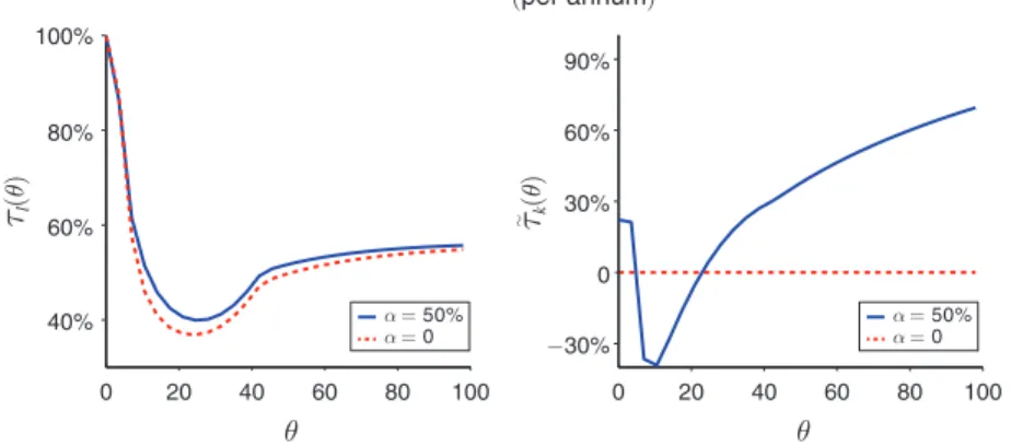
for a cali-brated version of our model. We refer to online Appendix C for a detailed description of the chosen parametrization, and here note only that we assume a fully equalizing reform threat with α = 50 percent and normally distributed taste shocks.23 Panel Ain Figure 2 shows the resulting optimal labor income tax rates (for wages up to $100/hour) both under full commitment ( α = 0 ) and when the political constraint (NR) binds. Panel B shows the optimal annualized marginal capital tax rate τ ̃ k (θ) on
the net return to saving for both cases.
As can be seen from the graphs, the labor tax schedules are very similar under full commitment and limited commitment, confirming that the key effects of the politi-cal economy constraint are on the intertemporal margin. Both schedules exhibit the typical U-shaped pattern emphasized in Diamond (1998) and Saez (2001), which is driven by the phase-out of the lump-sum transfer for low wages and by convergence to the asymptotic marginal tax rate due to the Pareto tail for high wages. Panel B demonstrates the U-shaped pattern for the marginal capital tax rate emphasized here and predicted in Section IIIA. In particular, marginal capital tax rates are negative for intermediate wages and positive otherwise (and of sizable absolute amounts).
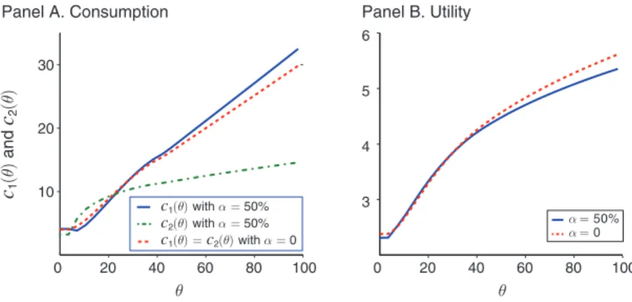
The underlying consumption and utility schedules are illustrated in Figure 3. Panel A shows consumption in both periods. While c 1 and c 2 coincide under full commitment (as shown by the dashed line for α = 0 ) because we set βR = 1 , they
23 In online Appendix C, we also show how the optimal allocation can be implemented by offering nonlinear
labor and capital tax schedules.
0 20 40 40% −30% 30% 60% 90% 0 60% 80% 100% 60 80 100
Panel A. Marginal labor income tax
τl
(θ)
θ
0 20 40 60 80 100
θ
Panel B. Marginal capital income tax (per annum) α = 50% α = 0 τk (θ) ∼ α = 50% α = 0
are distorted when the threat of reform is binding. In particular, the marginal cap-ital subsidy increases c 2 (the dash-dotted line) for intermediate wages in order to increase political support for the status quo to 50 percent of the population (from 42 percent under the full commitment solution).24 Of course, this must lead to an
aggregate welfare loss, which here is equivalent to a 2.1 percent consumption drop for everyone in both periods compared to the full commitment solution. However, there is considerable heterogeneity in how this welfare loss is distributed across the population. As shown in panel B, types with intermediate wages benefit from the presence of the political support constraint, whereas all other types lose. This illus-trates how our model can generate a pattern of redistribution where the middle class actually benefits from political constraints—rather than just having their consump-tion backloaded—which is again consistent with Director’s Law.
Do our numerical and analytic results find any reflection in real-world wealth redistribution policies? As noted by FSWY, policies such as income, estate, and wealth taxes, as well as the tax treatment of retirement accounts and subsidies to savings and education by the poor and middle class, all contribute to the progres-sivity of capital taxation. However, policies like tax-favored retirement savings pro-grams (where the tax subsidy is increasing in the marginal income tax rate up to a cap), the mortgage interest deduction (which subsidizes the accumulation of hous-ing wealth), and savings subsidies for college education, tend to be targeted more directly at middle-class voters than at the very poor.25 Moreover, means-tested
gov-ernment transfers can lead to an overall U-shaped pattern of marginal capital taxes. For example, in the United States, only individuals with sufficiently few assets qual-ify for Medicaid or Federal Student Aid, and only individuals with sufficiently low investment income qualify for the Earned Income Tax Credit. These asset tests can lead to positive marginal savings taxes for the poor. More generally, the contribution to capital tax progressivity of subsidies to savings and education by the poor are at
24 Aggregate consumption in periods 1 and 2 remain roughly equal to each other.
25 Similarly, Doepke and Schneider (2006) show that the inflation tax effectively redistributes from rich,
bond-holding households to middle-class households with fixed-rate mortgage debt, consistent with our version of Director’s Law. 0 20 40 60 80 100 10 20 30 Panel A. Consumption c1 (θ) and c2 (θ) θ 0 20 40 60 80 100 3 4 5 6 Panel B. Utility θ α = 50% α = 0 c1(θ) with α = 50% c2(θ) with α = 50% c1(θ) = c2(θ) with α = 0
least partially offset by the phase-out of these subsidies, unless eligibility is solely determined by labor income. While we do not claim that these patterns are neces-sarily driven by concerns for political stability—especially in the United States, where socialist threats have historically been less important than in Europe—they are consistent with our results.26
V. Conclusion
This paper has studied dynamic taxation under the assumption that a policy is sus-tainable if and only if it maintains the support of a large enough political coalition over time. Optimal taxes differ starkly from those in settings where the government is free of political constraints. Rather than predicting zero capital taxes as in the full commitment case, our model predicts progressive or U-shaped capital taxes, so that saving is subsidized for the poor and/or the middle class but is taxed for the rich, recalling Director’s Law of public redistribution (Stigler 1970). For any progressive reform threat, U-shaped capital taxes are optimal if individuals’ political behavior is purely determined by economic considerations.
We have also investigated several extensions of the model. In online Appendix D, we consider a setting where the full commitment benchmark involves nonzero cap-ital taxes, and show that the pattern of capcap-ital taxes identified in our baseline model can then simply be interpreted as the optimal “addition” to this nonzero benchmark. We also show how our results extend from two periods to a simple overlapping gen-erations model, following FSWY.
Finally, in ongoing research we analyze a version of the model where the gov-ernment still lacks commitment across periods, but once in period 2 has the ability to strategically commit to a reform to the capital tax schedule.27 The “ no-reform”
constraint in this case is thus that the government must design an intertemporal pol-icy in period 1 that it itself will not be able to subsequently replace, with sufficient support among the citizens, by any more-preferred policy. In this variant, our main finding is that the progressive capital taxation result of FSWY is surprisingly robust, and in particular does not depend on the shape of the taste shock distribution. Taken together with our results here, this suggests that the nature of potential political reforms is an important determinant of the progressivity and middle-class bias of capital taxes, and consequently of the long-run distribution of wealth.
Appendix A. Proof of Proposition 1
Recall that the government’s problem is max c 1 , c 2 , y ∫ v (θ) dG subject to (RC) , (IC), and (NR′ ). Any solution to this problem must also must solve the dual problem
min c
1 , c 2 , y
∫
( c 1(
θ)
+ 1_
R c 2
(
θ)
− y(
θ)
) dF26 For another explanation of such savings distortions, see Golosov and Tsyvinski (2006). 27 See Scheuer and Wolitzky (2014) for a preliminary analysis.