Application of linear routing systems to regional groundwater problems.

APPLICATION OF LINEAR ROUTING SYSTEMS TO REGIONAL GROUNDWATER PROBLEMS

by

Donald Hilton Evans B.S., University of Colorado

(1966)

Submitted in partial fulfillment of the requirements for the degree of Master of Science in Civil Engineering

at the

Massachusetts Institute of Technology (September 1972)

Signature of Author. . . . . Department of Civil Engineering, September, 1972

Certified by . . . ...

Certified

Thesis

b

Supervisor

Accepted by . . ... . . . . Chairman, Departmental Committee on Graduate Students of the Department of Civil Engineering

ABSTRACT

APPLICATION OF LINEAR ROUTING SYSTEMS TO REGIONAL GROUNDWATER PROBLEMS

by

DONALD HILTON EVANS

Submitted to the Department of Civil Engineering on

August 29, 1972, in partial fulfillment for the degree

of Master of Science in Civil Engineering

Work in groundwater analysis goes back to the last century. Only in the last decade, however, has there been an increase of interest in applying a linear systems approach to the problem of routing ground-water flow. This thesis applies linear systems to the routing of

groundwater within a regional basin.

The research reported here has been devoted to the following: 1. Developing a fast convolution technique through the use

of the Fast Fourier Transforms.

2. Developing a method for determining the system response parameters through linearizing the governing equation for groundwater flow by applying Laplace transforms and using

the Method of Moments.

3. Developing a groundwater routing model using the above techniques applied to a regional groundwater basin. The results from the Harmonic Analysis have been compared with those generated by the complete solution for open channel flow.

The hydrograph generated with the use of the parameters determined from the parameter estimation technique are compared to those resulting from a finite difference scheme.

The techniques developed in the use of Harmonic Analysis and parameter estimation are incorporated into a model for analyzing a regional groundwater problem and the results discussed.

Thesis Supervisor: Brendan M. Harley

Title: Assistant Professor of Civil Engineering 2

-ACKNOWLEDGEMENTS

This work was supported financially by the Subsecretarla de Recursos Hdricos, Ministerio de Obras y Servicios Pblicos, Argentina. Administrative support has been provided by the M.I.T. Division of Sponsored Research through DSR 72817. All computer endeavors were accomplished at the Information Processing Center, M.I.T..

The author wishes to extend sincere gratitude to Professor Brendan M. Harley of the M.I.T. Civil Engineering Department, who, in supervising this thesis, provided assistance and guidance for this research.

The support received from Mr. Rafael Bras, M.I.T. graduate student, in the development of the Harmonic Analysis section of this work is gratefully appreciated.

Additional appreciation goes to Mr. Dario Valencia and

Mr. Guillermo Vicens, Research Assistants for their helpful ideas gen-erated through enlightening discussions. Also to Miss Elba Rosso for enduring the dreadful script in the typing of this thesis, and to Mr. David Njus, graduate student, Harvard, who as penman and scholar, with careful thought, drafted the figures herein.

Finally but not least, thanks goes to my wife, Rosemary, and our daughter, for the loneliness endured during the period of this thesis.

TABLE OF CONTENTS Page Title Page 1 Abstract 2 Acknowledgements 3 Table of Contents 4 I Introduction 7

I-1 Problem Statement 7

I-2 Background to Groundwater Flow Modeling 8

I-3 Introduction to Linear Systems 9

I-4 Scope of Work 10

I-5 Brief Summary of Results 11

II Developments to Linear Systems Analysis 12

II-1 Hydrograph Theory 12

II-2 Linear Systems 14

II-3 Some Typical Systems 16

II-3.1 Linear Reservoir Model 17

II-3.1.1 Application to Time Varying

Inflow 20

II-3.2 Linear Channel Model 22

II-3.3 Two Parameter Models 22

II-3.4 Three Parameter Models 25

II-4 Model Formulation Using Linear Systems 25

II-5 Groundwater Systems 28

II-6 Parameter Estimation 34

II-7 Theoretical Development to the Regional

Ground-water Routing Model 41

III Fourier Transforms in Linear Hydrologic Systems 46 III-1 Introduction to Fourier Analysis 46

III-2 Fourier Transform Technique 48

III-2.1 Characteristics of Subroutine FOURTRAN--Numerical Integration Technique 49

III-2.1.1 Test and Results for

Sub-routine FOURTRAN 50

III-2.2 Characteristics of Subroutine

FOURT--Fast Fourier Transform Technique 56 4

-Page

III-2.2.1 III-2.2.2 Data Requirements

Subroutine FOURT--Forward

Transform

III-2.2.3 Subroutine FOURT--Inverse Transform

III-2.2.4 Implications of the Input-Output Requirements

III-2.2.5 Tests and Results

III-3 Selection of an Efficient Fourier Transformation Technique

III-4 Convoluting with Fourier Transforms

III-4.1 Defining the Nyquist Frequency, o III-4.2 Effects of Complex Responses on the

Nyquist Frequency

III-4.3 Selection of Response Function Duration

III-4.4

Selection of the Output Period

III-4.5

An Example-The

Theoretical Solution

III-4.6 Obtained Results

III-5 Application to Surface Routing IV Application to a Regional River Basin

IV-1 Discussion of the Selected Regional River Basin IV-l.1 Geology and Soil Description within

the River Basin

IV-1.2

Hydrologic and Agricultural Discussion

IV-2 Conceptual Discussion of a Regional Groundwater

Routing Model

IV-3 Model Development

IV-3.1 General Linear Groundwater Routing

Model

IV-3.1.1 Discussion of the Shallow Zone System Implemented into the Model

IV-3.1.1.1

Drainage Spacing

IV-3.1.1.2 Finite

Differ-ence Scheme IV-3.1.1.3 Parameter

Esti-mation with the Use of Finite

Difference

Scheme

IV-4 Linear Groundwater Routing Model Discussion IV-4.1 Model Results

56 56 57 57 57 58 58 61 64 65 67 69 71 74 83 83 83 86 87 90 90 102 103 104 105 107 112

V Concluding Remarks V-1 Summary V-2 Conclusion V-3 Future Work References List of Figures List of Symbols List of Tables Appendices A-1 A-2 A-3 B-1 B-2 B-3 C-1

Model Generated for Harmonic Analysis Fast Fourier Transform Program

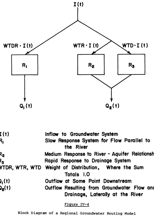
Groundwater Routing Model

Procedure for Determining the Time Period for the Nash Model

Derivation of the System Response to a Delta Function

Method of Moments-Parametric Analysis Computer Implementation of the Convolution Technique by Means of Harmonic Analysis

6 -Page 139 139 139 142 143 150 154 162 163 163 167 173 181 184 189 193

Chapter I

INTRODUCTION

I-1 Problem Statement

The theory to groundwater flow representation goes back to 1856 when Henry Darcy first developed an empirical relationship for steady-state saturated flow. Jules Dupuit and many others have since expanded Darcy's relationship into one representing unsteady condi-tions. Through expanding knowledge in subsurface hydro-geology and soil mechanics, the complexities of the subterranean region have become enormous. The 'real world' conditions which are

non-homogeneous, non-isotopic and contain cracks, fissures, etc., make it impossible to represent, in detail, the behaviour of a subsurface environment.

The complexities of the subsurface terrain also implies that the response of such a system is non-linear. However, if the

neces-sity of a non-linear solution is accepted, a unique solution for each soil condition, recharge pattern and the many other facits of the

system is required. Thus, with the linear systems approach of modeling the groundwater system, we desire to find a simple but

functional procedure for determining the general behaviour pattern of such a system. This theme will be further discussed in Section I-3.

I-2 Background to Groundwater Flow Modeling

Over the past decade, a tremendous effort has been devoted to the understanding of groundwater flow. The techniques vary widely but may be categorized into theoretical, analytical, experimental and numerical. Initial attempts were theoretical, going back to the early

1900s, when the dispersive effects of the groundwater systems were noticed. Since that time researchers have delved more deeply into the relationship of the various subsurface parameters to the dispersive effects caused by the soil characteristics. Breitenbach [1971], in a paper presented on groundwater simulation, pointed out the various analytical techniques used to-day. These analysts use Fourier

Series, Laplace Transforms, conformal mapping or graphical approxi-mations. The data are obtained, generally, by methods of well withdrawals or parallel drains of a variety of configurations.

Simulation techniques used, range from physical models using sand or other porous media, viscous fluids, electric means (relating Ohm's Law to Darcy's Relationship) and membranes, to numerical

methods. It is interesting to note that many modern methods or

theories have developed from other fields of study, for instance, the well known heat flow (Carslaw and Jaeger (1959)) relation to dis-persion, as well as Ohm's Law in electrical theory to mass flux

(Darcy's Law). The background and theory involved in these areas are discussed by Reddell and Sunada [1971].

8-A Frenchman by the name of D'8-Andrimont introduced concepts which lead to simulation of small groundwater basins by Toth [1962] and Freeze and Witherspoon [1966]. With the advent of the digital computer came a rapid increase of basin studies, for example, those done by Bittinger, et al. [1967] and Tyson and Weber [1964] as well as many others.

As the vastness of groundwater storage reservoirs unveils, researchers are beginning to widen the scope of subterranean flows to

a regional basin. Nelson and Cearlock [1967] discuss the various methods applied to large heterogeneous systems. Schneider [1966] and Megnien [1964] also have done work in analysing regional flow patterns of groundwater.

I-3 Introduction to Linear Systems

As many researchers turned to numerical methods in an attempt to by-pass the complexities of the analytical solutions for computing the reactivity of a groundwater system, so have many turned to the linear systems approach. Originally, linear systems were developed for overland flow and were accepted in groundwater because, to quote Kraijenhoff Van De Leur [1966], "... the unit hydrograph methods are in complete accord with the nature of the simplifying assumptions that have been accepted in order to find analytical solutions for the

equations describing the flow of groundwater."

-9-The linear systems approach to routing groundwater in the subterranean region is a subset to work done by Sherman [1932], who advanced the unit hydrograph theory which later was used in routing of surface flows. It was an attempt by hydrologists to estimate the

overall effect of an 'ideal' system and compare the result to an actual system. The hope was that a close approximation to that system would be obtained. The basic assumption underlying linear system theory is that the series of simple inputs may be used in conjunction with a characterizing function of the system to simulate the effects of a complex inflow pattern. Obviously, then, the characterizing function must implicitly contain all the variable process characteristics neces-sary for such a representation - an ideological condition to be sure. Should such a simplifying technique be used at all? A good justifica-tion for using linear systems is provided by Rodriguez [1972] when he says that a linear system "... may provide less information where information is not wanted and better information where it is wanted, all at less cost in time and effort."

The work that has evolved from linear systems in groundwater flow can be found in Chapter II.

I-4 Scope of Work

The work carried out in this thesis will be:

-a) to develop the use of Harmonic Analysis within the linear systems approach for a fast computa-tional scheme of convolution,

b) To use this method to develop a general model that can be used under regional consideration,

c) to apply the model to a regional area.

I-5 Brief Summary of Results

A convolution technique is discussed in Chapter III which utilizes a Fast Fourier Transform program developed at M.I.T.. This procedure was found to be highly efficient in terms of time and

accuracy. In Chapter IV, a groundwater routing model is presented which is capable of utilizing any configuration of system response which

might be encountered in a groundwater zone. This model utilizes the convolution technique in an effective procedure for analyzing such a groundwater system. In application of this model it was found to be better practice to isolate the different flow processes discussed in Chapter IV since the substantial damping effect of the groundwater

aquifer produced time steps incompatible for aggregating those pro-cesses into one outflow hydrograph. Use of the fast Fourier transform technique for predicting the response to an input provides a highly efficient procedure for analysing both the transient and the periodic situations. This is found especially useful in studying the behavior of slowly responding aquifer systems to periodic inputs.

-Chapter II

DEVELOPMENTS TO LINEAR SYSTEMS ANALYSIS

II-1 Hydrograph Theory

In 1929 Folse presented the ideas of base-flow separation, reduction of rainfall due to the variance of infiltration rates and the derivation of physical constants for representing hydrologic

systems. Sherman, in 1932, used these ideas to develop the well known hydrograph theory. The basic assumptions for use with the unit

hydrograph which is the result of surface runoff or effective rainfall,

are:

a) Effective rainfall is uniformly distributed within its duration.

b) The effective rainfall is distributed uniformly over the entire drainage basin.

c) The time duration is constant for a direct runoff hydrograph due to an effective rainfall of unit

duration.

d) Those direct runoff hydrographs that have the same time duration have ordinates which are directly proportional to the total amount of direct runoff represented by each hydrograph. Note that this

-implies use of the principles of linearity, superposition and proportionability.

e) The runoff hydrograph from a given rainfall period reflects all the physical characteristics of the given drainage basin.

The two significant features in linear systems application that are invoked by the above assumptions are those of time invariance and of superposition. Time invariance, i.e., stationarity with time, implies that the basin response will not vary with time - in other words, the resulting hydrographs of an effective runoff of the same duration will be the same. Superposition refers to the property that a hydrograph resulting from a given pattern of rainfall excess can equivalently be generated by superimposing the hydrographs from sepa-rate amounts of rainfall excess that occur during each period of the same duration. Thus, in order to use the principle of superposition only those systems that consist of linear elements may be considered. The most effective way of characterizing the behaviour of such systems

is to allow the effective input to become a delta input (or unit impulse). The resulting output is known as the instantaneous unit hydrograph, designated by h(O,t) or I.U.H. The properties are:

h(O,t) = 0 t < 0

h(0,t) + 0 t + 0

II-1

-h(0,t)dt = 1.0 = volume of runoff.

II-2 Linear Systems

A system, as defined by Eagleson, in 1967, is any set of inter-related components, material or conceptual, that are identified by their state variables. When the components are isolated from the

'real' system and provide the state variables, the result is an

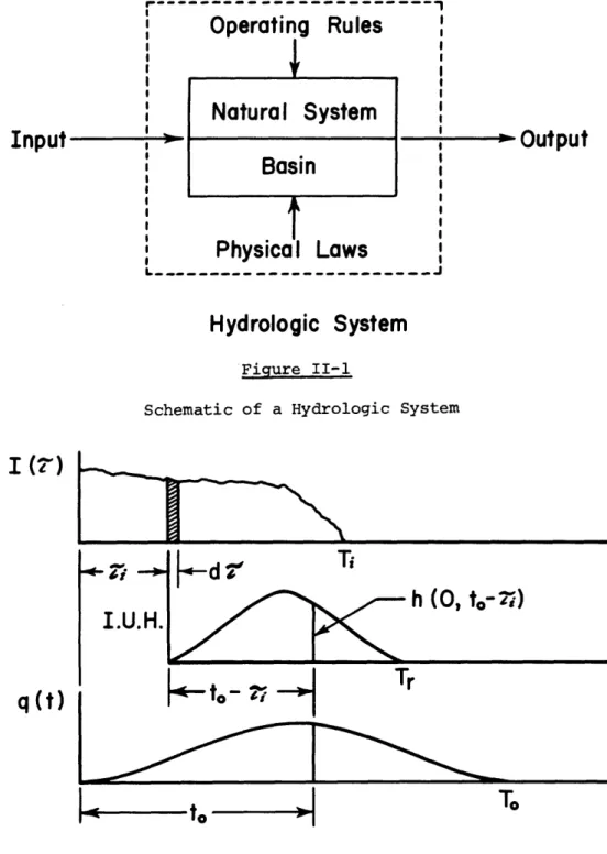
'idealized' system since it excludes some of the parameters or charac-teristics found in the environment. If this were not done, the task would either be impossible or so complex that it would be economically infeasible. A schematic of a hydrologic system might be as shown in Figure II-1.

The Instantaneous Unit Hydrograph, I.U.H., is the basis for the linear systems theory since it represents the response of a system to a unit impulse (delta function), and completely characterizes the system. The output resulting from the application of a known input can be uniquely determined by convolution of the input with the I.U.H.

The characteristic function of a linear system,e.g. the I.U.H., can be of two types, one being time invariant and the other being time variant. If the system is time invariant, then the system may be represented by a differential equation with constant coefficients as

-Operating Rules

_

Output

Physical Laws

I

Hydrologic System

Figure II-1

Schematic of a Hydrologic System

h (0, to-do)

Figure II-2

Linear System Approach in Deriving an outflow hydrograph

- 15

-Input

Natural

System

Basin

--

i

I.U

q(t)

L

a_.

_

.~~~~~~

t

-ICIIIII~~~~---~~~ I II II II I I I I I I I I I I I I I I I I I U- 1 I I I I II I II II I

in Equation II-2.

d n

ni

d

n - 1

q(t0

I(t)

= An q(t)

n dtn n- dtn -1

II-2 where I(t) = Time varying input

q(t) = Time varying output

This equation implies that the response to a sum of inputs is the same as if the inputs were individually computed and the responses summed. The difference between a time invariant system and a time variant system is that the coefficients for a time variant system are time dependent. The behaviour of a typical L.T.I. (Linear Time Invariant) System is shown in Figure II-2. This figure also represents the use of the convolution integral (or Duhamel's Integral) for a causal system, viz

q(t) = I(T) h(t-T) d II-3

0

where I(T) = Inflow Rate

h(t) = System's impulse response function

II-3 Some Typical Linear Systems

Previous sections have discussed the use of a characteristic function which when convoluted with simple inputs will produce an output hydrograph representative of the system. This characteristic

-function may consist of one, two or three parameter models that are used to represent the system responses to an input function. The

following sections describe the basic models that are presently used in representing a linear system response.

II-3.1 Linear Reservoir Model

In a groundwater system, one would normally expect hetero-geneous soil conditions, as well as extremely small (in relation to those found in surface hydrology) transmissivities or diffusivities. Therefore, one might assume that the translational effects of

sub-surface flow might be neglected and treat the system as a storage reservoir. The reservoir is what is known as a one parameter model where the one parameter, K, is used to represent the total hydraulic

characteristics of open channels for surface flow routing or the soil characteristics for groundwater flow. The conceptual storage reser-voir is shown in Figure II-3. The linear storage is related to the outflow by:

S = K q(t)x II-4

where x = 1 for linear systems < 1 for sublinear systems > 1 for supralinear systems

The continuity equation for the storage reservoir is given by Equation II-5, where x = 1.

o

0

4-0

rC =I 4-0*

4-~~~~~~~~~~~

0 0 0 _UQw 0 m

0

11I)

* H i-kl k C) w o4-- 0

6

U

4-H-

_ 4-%.O

-

18

-0

'4-c

I(t) = q(t) + dt

I(t) = q(t) + K d q(t)

dt

II-5

where S(t) = represents the reservoir storage

K = time constant or lag between the input centroid and the output centroid

q(t) = rate of discharge

Equation II-5 can be rewritten as:

d q(t) + q(t) I(t)

dt K K II-6

This is a first order linear equation and the total solution may be determined from the homogeneous and particular solutions.

The complete solution to equation II-6 is given by

q = et/ [ I e t/K dt + C]

q~~~I

/

II-7

assuming a constant input, the complete solution becomes:

-t/K

q=C e

+

I

Introducing the boundary conditions which are: q = 0, t = 0 II-8 II-9 results in thus C1 e + I = 0 C1 = -I or - 19 -II-10 II-11

The complete solution-to a constant- inflow to a storage reservoir- then becomes

Q = I (1-e / ) II-12

II-3.1.1 Application to Time Varying Inflow

If we reservoir, the

as given by

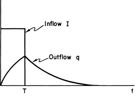
apply a constant input of rate I to such a linear resulting outflow rate is as shown in Figure II-4, or

q = q =

I

1 e

(t-T) K d T II-13 = I (1-et/K )

where t < T, the input time period of I.

If equal time the outflow rates, qn

periods are assumed with block inputs, I , then at the end of periods 1, 2, ... n, would be:

q = Ii (l-e -1/K ) q2 = I2 (-e -/K ) + I e -/K II-14 -I / -1/K

=I (-e )

n

+

I e

n-1

+

n- 2 2/K fl-2 - n-l K 20 -.... I e

I nflow I

Outf low q

t

T

Figure II-4

Outflow Hydrograph Resulting from a Constant Input to a Linear Reservoir

- 21

II-3.2 Linear Channel Model

Another single parameter model, known as the lag model or the linear channel, is used for the purpose of translation of a flood wave. The linear channel requires a constant velocity at any point in the channel for all discharges such that the relationship between the inflow and outflow at that point is merely:

Q (t) = I (t-T) II-15

where T represents the translation in time of the flood wave with no attenuation of the wave.

Dooge [1959] first presented the linear channel concept and pointed out that it can also be considered to be as a cascade of an

infinite number of infinitesimal storages. As shown in the above section, the lag to a single reservoir (single storage) is repre-sented by K. Then, if we have n reservoirs in series, the lag would be nK. Thus if n goes to infinity as K goes to 0, while nK remains

2

constant, the variance about the mean, nK , goes to zero, implying that an instantaneous input of unit input will cause an instantaneous output of the same volume after the mean travel time of nK.

II-3.3 Two Parameter Models

When considering a groundwater system, one must be realistic 22

-in choos-ing a model for represent-ing that system. Common sense tells us that a pure translation or the linear reservoir (exponential distri-bution) which lacks the property of having adequate 'memory' (Hillier

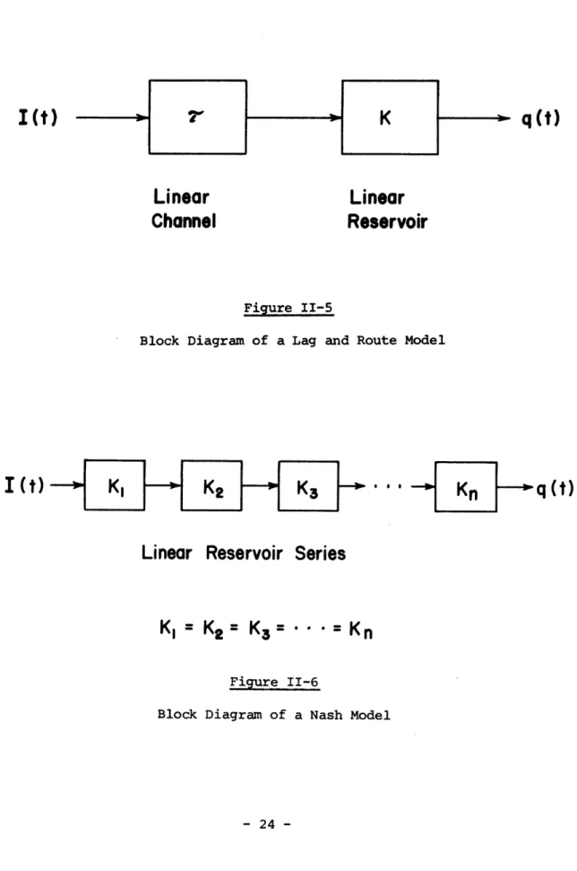
[1967]), will fail to represent the groundwater system. Thus the tendency has been to incorporate these elementary, single parameter models into a variety of configurations. This led to the two param-eter models such as the Lag and Route Model or the Nash Model. The former is represented by the block diagram in Figure II-5. It has the following impulse response:

q (t) = e K II-16

where K = delay time of the linear reservoir.

T = translation time of the linear channel.

Noting the obvious increase in flexibility by applying such models in series, Nash [1958] developed what has become known as the Nash Model - (Also developed by Kalinin - Milynkov [1958]). Nash

conceptually applied a series of n reservoirs each of delay time K, represented by the block diagram in Figure II-6, in order to repre-sent the systems I.U.H.. Thus the total lag to the system can be shown to be nK, since in a series configuration the outflow of one reservoir is the inflow to the succeeding reservoir. The impulse response for this model is:

Linear

Channel

Linear

Reservoir

Figure II-5

Block Diagram of a Lag and Route Model

I I KK -- K2 -- '

q (t)

Linear Reservoir Series

K,

= K2 = K3 = - . = Kn

Figure II-6

Block Diagram of a Nash Model

24

1 t n-i 1 -t/K

h (O,t) = (-) - e II-17

K K I(n)

Notice that the Nash Model is also a modified gamma distribution. Nash simply used the tools developed earlier by Zoch [1934] in linear reservoirs, Clark [1945] in linear storage routing and Edson [1951] in two parameter model development.

II-3.4 Three Parameter Models

Many three parameter models merely add the linear channel, a translational effect, to the two parameter models. In this paper this

is accomplished with the Nash Model as discussed above. However, Harley [1967] also uses the translation with a Muskingum Model, and the Diffusion Analogy.

The advantage of the three parameter models is that they are more capable of simulating a complex system as in the natural highly damped groundwater system.

II-4 Model Formulation Using Linear Systems

With the basic tools now available to linear systems re-searchers, an infinite number of configurations become available to represent the complex systems of the real world. Many of the fol-lowing models were presented by Kraijnhoff [1966].

In 1955 Lyshede related a series of exponential functions to the effect of runoff from rainfall and the basin characteristics. This pointed out the possible use of linear reservoirs in series which form the cascade effect of the Gamma distribution.

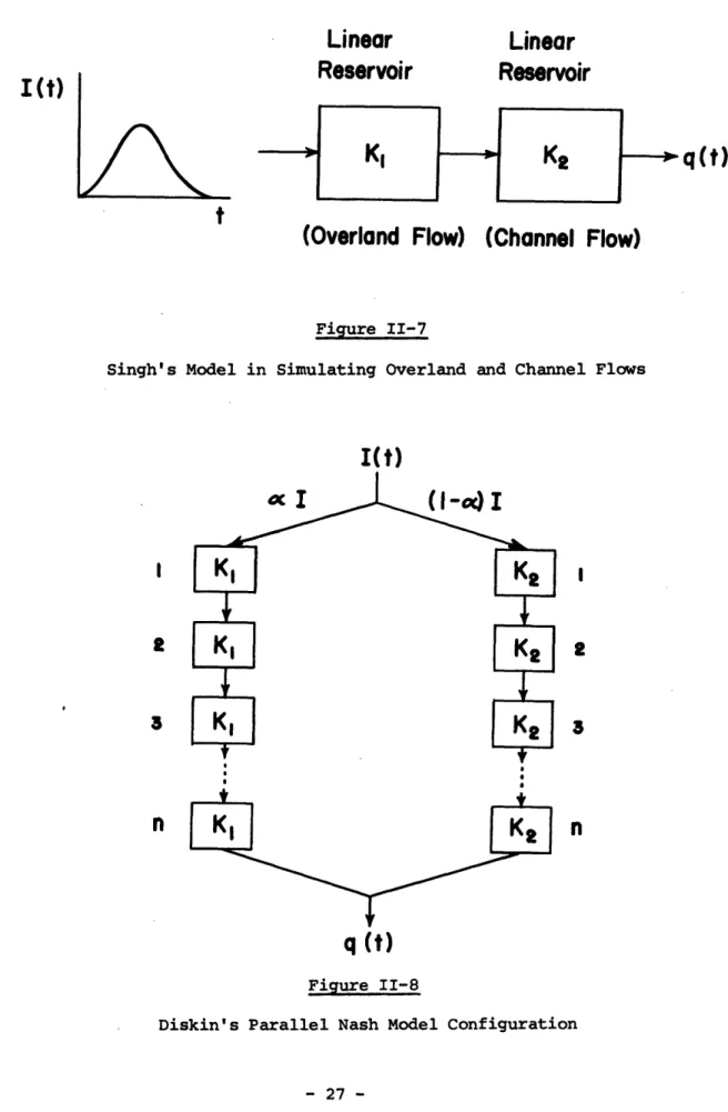
Singh, in 1964, used the time - area hydrograph and routed it through two linear reservoirs in series to represent the effect of overland and channel flows. Singh's System is shown in Figure II-7.

Diskin, also in 1964, proposed a model using two Nash Models in parallel, each branch consisting of a different number of equal reservoirs and both branches having different lag characteristics in the reservoir series such as shown by Figure II-8. Thus by splitting the input hydrograph, Diskin was able to develop a system that would lag the output by:

a n K1 + (1-a) n K II-18

The I.U.H., of this system then would by represented by

h (Ot) a t )nl -1 -t/K1 + Kl(nl- 1) Kl II-19 (1-a) t n2 - e -t/K2 K₂ (n2 - 1) K2 26

-Linear

Reservoir

Linear

Reservoir

(Overland Flow) (Channel Flow)

Figure II-7

Singh's Model in Simulating Overland and Channel Flows

I(t)

Co c 3 n

(I-c) I

6 6 I

3

n

q

(t)

Figure II-8

Diskin's Parallel Nash Model Configuration

I(t)

II-5 Groundwater Systems

The Netherlands has done work in groundwater systems for many years using the Dupuit - Forchheimer approximations.

As mentioned in Chapter I, there was skepticism in using a linear system approach until it was realized that the basic assump-tions for analytical soluassump-tions to groundwater flow were equivalent to those used in the unit hydrograph theory. Therefore, the

development stages of groundwater flow in linear systems are described briefly in the following paragraphs.

In 1947, Edelman developed equations for two dimensional groundwater flow into a unit length of channel and applied the

convolution integral to determine the effect on the groundwater flow-rate of a constant infiltration flow-rate into the phreatic zone as shown in Figure II-9, resulting in the equation

1

Q (t) = -P KD (t-T) 2 d (-T)

II-20

p 2 t 2

where P = constant percolation rate

KD = transmissivity

-y

=

Initial Saturated Zone Thickness

P

=

Constant Percolation Rate to Phreatic Zone

qx

=

_{Unit Flow at x}

Q(t)

=

Outflow Rate at Channel

,

=

Active Porosity

p

I

Figure II-9

Edelman's One-Sided Groundwater Flow to a Unit Width Channel

I(t)

q (t)

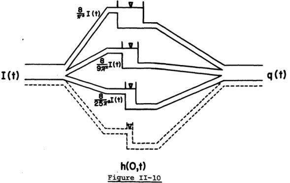
h(O,t)

Figure II-10

Reservoir Representation of Kraijenhoff's Flow to Drainage Canals 29

1P = active porosity

In studying the effects of the phreatic zone in irrigation areas, Glover [1954] developed an equation which relates the spacial and time change of the free water surface to an instantaneous irri-gation inflow, s, in equation II-21

s 4 1 e-n t/j nl1x

y(xt)

=

-

-

--

n--/e

sin

IT n L

n=1l,3,5

II-21

where j iL 2

=- KD

From this relationship, Kraijenhoff [1958] developed the I.U.H., for flow into parallel drainage channels.

h (,t) e-n2/j II-22

n=1,3,5

Expanding and setting the lags, K, equal to functions of j, results in 8 1 -t/Kl 1 8 1 e -t/K2 + h(O,t) = - e +---e -2 K1 9 iT2 K2 II-23 1 8 1 -t/K ₃ 25 12 K3

We may see that this equation represents the behaviour of a system of linear reservoirs in parallel as shown in Figure II-10. The lag for such a system is given by equation II-24.

-LAG = 7 K1 + 9 2 K2 +.. 8 1 1 -24 = j (1+ +

~2

34

4

54

.. .) II-24 12 8 4 2 =72 96 12 where K1 = j; K2 = j/9; K3 = j/25 etc.

De Jager [1965], Wesseling [1969] and Wemelsfelden [1963] used other modified configurations to represent flows to parallel drains or

river channels.

In an attempt to develop the use of linear systems in ground-water application, Dooge [1960] used the concepts introduced so far

to derive coefficients in a simplifying technique. By accepting the work- done by Thornthwaite and Penman in estimating infiltration,

evaporation and other soil characteristics that determine the flow of groundwater in the unsaturated zone, Dooge developed coefficients for use under a number of conditions, these being:

a) Water table close to the surface where there is a direct effect on recharge by rainfall and evapotranspiration.

b) Water table well below the ground surface where the recharge to the groundwater system is

reaches field capacity.

c) Composite type where the groundwater table reacts as a shallow table until the groundwater 'storage' decreases producing an effect more in line with a deep water table.

Dooge's procedure is based on a constant recharge over a given time period. Using constant time periods and the storage

concept generated by the linear reservoir discussion in Section II-3, he derived three routing coefficients and three coefficients required

under the conditions of negative recharge. These basic equations are

Qn = C Rn + C1 R_1 + C2 Qn-l II-25

where Q = Outflow due to contributions by the past n recharges R = Recharge in period n

n

Rn_1 = Recharge in period n-1

Qn-I = Outflow due to contributions from the past n-1 number of recharges.

The coefficients are given by:

C

_C

=1

_{1- K}

K (1 -T/K

o T

-K -T/K e-T/K

C1 = - (1-e ) - e

T -T/K

C2 = e

where T = time period of the recharge.

K = the linear reservoir lag coefficient.

The negative recharge computation is based on a storage calculation at the end of period n, viz

S = R - (1-eT/K ) + (Q - C R ) 1

n n T n n T/K_1 II-27

If for any period this goes to zero, he calculates two additional coefficients: S = C3 R + C4 Q n n n II-28 K 1 where C₃ = T eT/K_1 1 C4 = eT/K_1

Thus if one knows the parameters required by linear reservoir theory, simplified coefficients may be calculated for routing through a ground-water system.

Though the computation scheme would become more complex, one could conceptually consider using a time varying period that could be accepted as being more realistic, i.e., to maintain a constant

input, which is acceptable under certain restrictions, and vary the time over which the inflow is constant.

II-6 Parameter Estimation

Definitions, derivations and configurations have been offered in the previous sections but the most important and perhaps the most significant aspect to linear systems theory is that of parameter estimation. It should be obvious that a simulation proce-dure requires a highly selective method of correlating the I.U.H. parameters as dependent variables with the basin characteristics as

the independent variables. Methods available for parameter esti-mation include:

a) Fourier Coefficients. b) Laguerre Coefficients. c) Method of least squares. d) Method of maximum likelihood. e) Method of moments.

f) Wiener - Hopf equations

O'Donnell [1960] presented an approach to develop the I.U.H., by means of Harmonic Analysis, which produced Fourier Coefficients.

-He used the fact that the Fourier expansion can be used if the input/ output hydrographs are assumed periodic. These expansions may be

represented by Inflow Expansion: oo =

a

Cos

(n-

T) + n T n=o oo b sin (n -) n= n n= 1 I.U.H. Expansion: h (t-T) = 0o co C

a

os

(m

2(t-T)) +

I

sin (m

27

(t-T)

m T

m

T m=o m=1 Outflow Expansion: Q (t) oo co = A Cos (r 21T + B sin (r T-) r= o r r= r r=o rM 1 II-31

By applying the convolution integral and considering the n

harmonic, he was able to derive the kernel coefficients with respect to the input/output coefficients, thus giving:

A 1 o a = - m

o

T a

o

a A +b B

2 nn n n = - for n 1 n T a 2 + b 2 n n II-32 I (T) II-29 II-30

a B -b A 2 n n n n

n

T a

2

+

b

2

n n

Thus, if a long enough record is available and accurate, then a simple means for determining the instantaneous unit hydrograph is available.

Dooge [1965] proposed another scheme for the analysis of heavily damped linear systems using Laguerre functions, similar to the method proposed by O'Donnell [1960] in using coefficients derived by means of harmonic analysis. The equations derived by means of the Laguerre functions are:

Input function 00 I (t) = I a

_nn

f (t) II-33 n=o Response function 00 h (t) = I a f (t) II-34 n n n=o Output function o0 Q (t) = I A f (t) II-35

n n

n=o 36

-The linkage function coefficient are given by

P

p-1

P=

O%

a

p-k -

a

p--k

II-36

k=o k=o

Eagleson [1965] presents the Methods of Least Squares and the Weiner - Hopf Equation as procedures for determining the instanta-neous unit hydrographs, while Hillier and Lieberman [1967] present the method of Maximum Likelihood and others in determining parameter estimators.

The Method of Moments for estimating parameters was first applied to hydrologic systems by Nash [1959]. The accuracy of this procedure is dependant on the number of samples taken of the system and that these samples are truly representative of the basin charac-teristics. Maddaus [1969] offers what he considered to be disadvan-tages to the use of this method, and are as follows.

a) Non-linearity is filtered out of the lower moments but the non-linearity tends to concentrate in the higher moments.

b) Inconsistency may occur between the parameters and the assumed model resulting in negative parameters.

c) They tend to be biased at the extremities, thereby causing the greatest error at the peak.

-Since the Method of Moments is an effective parameter tech-nique in hydrologic systems, where our concern is with the lower

moments, then any non-linearities of the natural system must reside in the upper moments. When applying this procedure to unit hydrograph theory where only positive causal systems are considered, any

inconsistency producing a negative parameter would, indeed, reduce the effectiveness of this procedure. The effect of c) will be shown in Chapter IV where the peak is shown to have the greatest error when utilizing the Method of Moments. Since the lower moments do provide the more significant results in modeling hydrologic systems, it has become an accepted fact that the first three or four moments only, be used in parameter estimation. Nash [19591 recommends the use of dimensionless parameters in allowing an independence between the parameters and the I.U.H. This is accomplished by dividing all moments exclusive of the first by the first moment. To present an example of the Method of Moments, the Nash Model will be considered. The I.U.H. of a Nash Model may be represented by:

h (O,t) = (t/K)l et/K II-37

where n = number of equal linear reservoirs in series

K = the time constant or lag of a single reservoir.

-Then the first moment about the origin, or lag of the system is given by:

Ioo

0o h (O,t) t dt = nK K _{(t/K)n 1 e d (t/K)}

(n)

II-38 = n K

where M = first moment about the origin.

The variance, is

second moment about the mean (or centroid) known as the determined by the equation:

M2 = M2 -where M2 h (O,t) t2 dt 0 = K2 n (n+l) then II-39 M2 = K 2 n2 + K2 n - K2 n2 = nK2

where M1 = first moment about the mean

-M₂ = second moment about the mean

M2 = second moment about the origin

By the same procedure, the third moment (Skewness) and the fourth moment (Kurtosis) may be derived to be:

M3 = 2 n K

3

II-40

M = 6 n K4

A similar procedure may be used for the moments of the Linear Reservoir and Lag and Route Models. These are represented by Equa-tion II-41 and II-42.

Linear Reservoir Moments

M1 = K M2 = K2

II-41

M3 = 2 K 3 M4 = 6 K4

Lag and Route Moments

M = T + K

M2 = K 2

II-42

-M3 = 2 K3

M = 6 K4

Appendix B.3 develops moments in greater detail.

Another parameter that sometimes proves important is the time to peak, which is found by taking the first derivative of the I.U.H., and equating to zero,since in hydrology the work is with causal systems. Thus:

The time to peak is that at which

d h(O,t)

dt = 0 II-43

Then for the various models discussed in Section II-3:

Nash Model

Single Reservoir

T = (n-l) K

T = 0

P

Lag and Route Model T = T

P

II-7 Theoretical Development to the Regional Groundwater Routing Model

The basic equations for unsteady one dimensional flow will be considered assuming the following conditions apply:

a) Unconfined flow

b) Incompressable fluid flow c) Darcy's Law applies

d) Sloping bedrock

The continuity equation is given by:

ax

where

ah

qi

Sc

-

= -A

at

Ax

qi = inflow Ax = area of inflow Sc = storage coefficient h = piezometric head However, desired such that

the response to a Dirac delta function of inflow is the continuity equation will be:

a + Sc a = 0 t > II-46

The groundwater flow will be represented by a modified form of the Darcy equation, incorporating the advective velocity, as in Equation II-47.

q = a - K h h - II-47

p m

ax

42

q = groundwater flow (L3/T)

a = advective velocity due to the sloping

bedrock (L/T) h = piezometric head (L) K P h m = permeability (L/T)

= mean depth of the saturated water zone

The advective velocity may be more adequately shown to be

a = - K dh from Darcy's Law p dL

II-48 = - K . slope

P

where the minus sign indicates the direction of flow. Then equation II-47 can be rewritten as

a h h

,

ax

ax

pm

aX

and the continuity equation II-46 will then become

ah a2h ah a - K h - + Sc-ax p max2 at

= 0

II-50 or

K h

p m Sc

a

2

h

ax2 a ah Sc ax II-51 43 -II-49 where

By using Laplace Transforms, Harley [1967] shows that the resulting system response to the Dirac delta function input (of a similar relationship) will be:

h (x,t) = 2 1 * x .r (ct- x)2p

P t exp 4K P

thus equation II-51 results in:

h (x,t) = /

Sc

2 K nh p m 2 . x_{t3k exp (at/c-x)2} t 3/2 4 K t

6~

II-53

Appendix B.2 proves a similar result for a horizontal bedrock condi-tion.

The cumulants for the above response function are shown in Appendix B.2 to be derived simply from the Laplace Transform.

Harley [1967] shows the first four cumulants to be given by Equa-tions II-54

Cl = x/c

2 K x C2 = C_C3 II-54 44 -II-52

12 K2

x

C3 = C5 120 K 3 x = C7

Equations II-55 are the four cumulants derived from the governing equation of groundwater flow.

Z = x Sc/a Z2 = 2 K h Sc2 x/a3

p m

II-55 Z3 = 12 K 2 h 2Sc3 x/a5 p m Z = 120 K 3 h 3 SC4 x/a7 p m

In Chapter IV, the first three cumulants will be used to determine the lag of a single reservoir, the number of single reservoirs as well as the lag, T, required to simulate the system response based on the input parameters used to compute the cumulants shown above.

-Chapter III

FOURIER TRANSFORMS IN LINEAR HYDROLOGIC SYSTEMS

III-1 Introduction to Fourier Analysis

A linear system is characterized by the following equation:

fi() h (t-) d f (t) o III-1 where f. (t) h (t) f (t) o = an input function

= the system response function, characterized as the response to a unit impulse

= response of the system to the input f.(t)

1

Applying a Fourier transformation to equation III-1 yields

F ()

o f (t) e 0 t dt

III-2

e idt dt - f (T) h (t-T) d T

I i

Letting s=t-T and changing the order of integration, the above equation reduces to :

46 -r o 11r co 1 27r -0

co

F (W) = h(s) e

which can be further stated as

Fo(W) = H () F (( 0 1 where F. (w) H (W) F () o III-3 d s 21 I_ 27 0 III-4

= the Fourier transform of input function

= the Fourier transform of the system response, (multiplied by 2)

= the Fourier transform of the output.

Therefore a convolution integral can be reduced to a simple multiplication of Fourier transforms.

Traditionally in hydrology the whole series of linear models, such as the linear Reservoir, Muskingum, Nash and linear solutions to the momentum and continuity equations, have been utilized by obtaining

expressions for the system response function and performing the lengthy and time consuming numerical (or sometimes analytical) convolution in a computer.

47 -4)

The purpose of this chapter is to combine the knowledge of the analytical Fourier transforms of these linear systems with the availability of numerical computer techniques to obtain Fourier

transforms in order to utilize equation II-4 to find the outflow from a system resulting from a known inflow.

By reducing the complicated convolution procedures to a simple multiplication and by utilizing an efficient numerical trans-form scheme the time required to obtain the output function should be reduced significantly.

In this chapter two available computer programs to carry out Fourier transformations are investigated. One is based on traditional finite numerical integration of the Fourier transform equations; the other is based on the theory of Fast Fourier Transforms. The accuracy, speed and ease of use of each of these programs are evaluated and

compared.

III-2 Fourier Transform Technique

Two numerical, computational techniques are considered in this paper. One is based on the Cooley - Tukey Fast Fourier

Transform Theory which was available at M.I.T. as Subroutine

FOURT, (Appendix A-2). The other is based on finite numerical integra-tion of the Fourier Transform equaintegra-tion and will be noted by Sub-routine FOURTRAN (see reference Eagleson and Goodspeed (1970)).

-The discrete form of the finite transform used in Subroutine

FOURTRAN is:

1 NF

F () = - f(t) exp (-jw LAt) At III-5

L=1

where NF = number of points in time at which f(t) is given

f(t) = input function at interval At

At = time interval

W = angular frequency

This equation is evaluated at different equally spaced A's up to some cutoff frequency, w , which must be less or equal to T/At. If the given w0 value exceeds T/At it is automatically adjusted to this value. In order to return to the time domain (by taking the inverse transform) the procedure is as follows:

a) change sign of the exponential

b) integrate over the angular frequencies (Aw) c) evaluate at different times (t).

III-2.1 Characteristics of Subroutine FOURTRAN ---Numerical Integration Technique

The following are characteristics of Subroutine FOURTRAN: 49

-a) Two options are available to the user for the output, a complex spectrum or the normalized amplitude and phase of the spectrum.

b) The program does not require the input function to be periodic.

c) The input function is assumed to start at a value of zero,to be sampled at equal intervals,and to be zero after the sampled period.

d) For simplicity, the forward and inverse transform equation are made similar by multiplying by

1// 27, thus allowing a simple transition from the forward transform to the inverse transform.

e) Since the complex spectrum of a time series is symmetrical about the origin and if FOURTRAN is used to find the inverse transform, only one portion of the symmetrical transform is input and thus the resulting time domain series must be doubled in order to keep the proper scale.

III-2.1.1 Test and Results for Subroutine FOURTRAN

The tests performed on Subroutine FOURTRAN consisted of entering and exiting the program with one function in order to determine the effectiveness of the program in returning the iden-tical function. The function chosen was that of the linear

-reservoir as presented in Chapter II.

The forward and inverse Fourier transforms from Subroutine FOURTRAN are dependent on the following parameters:

At = sampling time interval

0 = maximum angular frequency, Nyquist frequency o

Aw = angular frequency interval.

Table III-1 is a tabulation of the significant parameters in the forward transform (frequency domain). In considering Table III-1 and comparing the analytical and computational transforms, these indicated:

a) Accuracy increases as the integration steps de-creased, i.e., At in the forward transform and AW in the inverse transform.

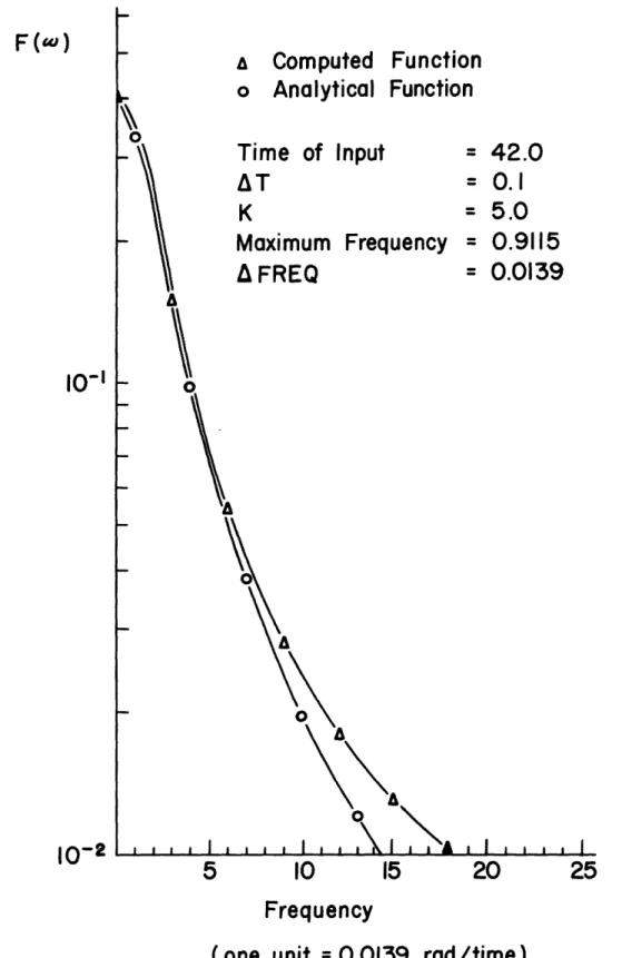
b) Figure III-1 shows the aliasing effect in the forward transform when compared to the analytical transform, i.e., as the transforms approach the higher frequencies, the complex spectrum obtained, using the program, diverges from the theoretical transform.

c) As the integrating variable, At, decreases the time of execution increases significantly. An

-00 'v L 4 ' C HA (N n co N Cl nr

r-m

v mn ) ("3) l H l o m l 0 a O

o0

* *

0

*

H

*

0

*

0

*

0

0

m m Cl OD co co

o

*

0

*

0

(N H-4 o 0 L Lin LO U) Lf Hl l rl r ( O3 03 oa 0' 0 Ln LA LA LA o i. Ln N o o or - rl

O

O

0

0

m m

o

o

LA Ln uL LA LA H H H H 'v l rl rl r blH N- N- N N N I C CN C N ul ur In in ur O O O O O O O O O O *n *n *n .n .n .n . . . LA Ln LA %. k k0 *r v LO rH N LA v N %9 H (N WD N LO (N H H H 0 H H H

J Jd J

J

J

J

o

o

0

0

0

0

0

0

0

Cl Cn m cl Cm C m m I V cli_H 0 0 U) H E-4

0

--H0

4j U)

U-x

~4

-H N E-< >1

u

)o aD rD

3

O rzI

z

35 I U) H E H 3 H U1 H li r EE-U)

z

E H 0

3H

F. < "I_la (d P: -.4 1I r:; -l > -O * OH u

3

. H -r- E-04-i 0 4

Oc

Z

P 4 EH E-L0 c) LA o0 Q4 -, U) P4 52

-a

Computed Function

-

Annlir',nl

lantirnn

=

42.0

= 0.1

=

5.0

ency = 0.9115

=

0.0139

I ,

I,

I, I

I

IlA I I I

5

10

15

20

25

Frequency

(one unit = 0.0139 rad/time)

Figure III-1

Aliasing Effect in the Forward Transform--Subroutine FOURTRAN - 53

-F(w)

o10-10-2

I UI M I IVI I

attempt was made to decrease the aliasing effect by increasing the Nyquist frequency, w ; as this decreased the integrating step, At, however the execution time again increased. Increasing A@, on the other hand, provides an inverse re-lationship with the execution time. The problem is that in order to provide good results in the inverse transform an adequate number of points in the frequency domain must be provided. This implies use of a smaller w and therefore higher execution times in the inverse and forward trans-form calculations.

The results obtained when finding the inverse of a complex spectrum using FOURTRAN are shown in Figure III-2. As the figure shows, the numerical integration method of finding the Fourier transform fails to reproduce its original input,. i.e., if a forward transform is

performed on an input and then the corresponding inverse on that trans-form, FOURTRAN fails to reproduce the original function. This is due to the finite integration technique. The problem that we are faced with is when a system response is to be represented by a series system

of models as discussed in Chapter II. In this case, the output of one model response is the input into the next, thus requiring a multiple

use of a convolution technique. Thus, if Subroutine FOURTRAN was

recalled a number of times, the integration error would compound itself. 54

-C -C

CO i

430

₀

_C

c 0

0

C)

E

Cd

d

55

-Q

(-too

II II

o

aio

I amI o O

0

E

Ew

o

(D t')

,-

E

0

Q) i I H H r_:

H1

.

1 O Ur E O4 zn (d E CM

III-2.2 Characteristics of Subroutine FOURT ---Fast Fourier Transform Technique

III-2.2.1 Data Requirements

This subprogram assumes periodicity, i.e., the input values represent one cycle of a periodic function. The input values must be at even time (frequency) intervals for a forward (inverse) transform and may be real or complex. However, when returning from the frequency domain the data must always be complex. If the number of data points is a power of two this subprogram will run at its maximum efficiency. The only data the program requires are the input values, the number of input values and information indicating if the inverse or forward transforms is desired.

III-2.2.2 Subroutine FOURT --- Forward Transform

The Nyquist frequency, o , is determined analytically as W/At, thus defining the frequency interval, Aw, at which the transform will be evaluated. A property of the FOURT returned forward transform is the symmetry of the transform about the Nyquist frequency, with that frequency as the midpoint (plus one if the function has an even number of points) of the transform. Since FOURT evaluates over a frequency range of 2(N-1)/NAt, at frequency intervals of 2/NAt, the Nyquist frequency will be located at point N/2 due to FOURT's symmetric repre-sentation in the frequency domain. The number of output points in

-Subroutine FOURT is identical to those input.

III-2.2.3 Subroutine FOURT --- Inverse Transform

The output of the inverse transform is a regular time series and has the same time intervals as the original input since it is

based on the same number of input points. The resulting time domain function must be divided by the number of points used in the calcula-tion in order to obtain the correct results- a property of FOURT. In finding the inverse transform the user must ensure that the complex spectrum is input in the symmetrical conjugate form described above.

III-2.2.4 Implications of the Input-output Requirements

As mentioned above, the number of points returned after transforming with the subprogram FOURT is the same as input initially. Since the program assumes a periodic function this implies that in using the program to convolute, by multiplication of input and response transforms, the same number of points must be in each of the transforms.

It is important to note that FOURT does not consider the 1/27 factor usually found in Fourier transforms so caution must be used in interpreting FOURT's results.

III-2.2.5 Tests and Results

In finding the inverse Fourier transform of a FOURT obtained 57

-complex spectrum, the program was able to reproduce the original time domain function identically, thus indicating a good computational scheme. When the theoretical Fourier transform was input in the fre-quency domain and the inverse was taken the results were very close to the true function, Figure III-3. However, the aliasing effect still exists as shown in Figure III-4.

III-3 Selection of an Efficient Fourier Transformation Technique

Subroutine FOURT, the Fast Fourier Transformation technique is chosen over Subroutine FOURTRAN for the following reasons:

a) it is considerably faster

b) the accuracy is maintained in the inverse trans-form when using the theoretical forward transtrans-form. c) the exact reproduction of the function in the time

domain is obtained when the forward and inverse transforms are computed in succession.

III-4 Convoluting with Fourier Transforms

Implementing the algorithm to convolute by multiplying Fourier transforms presents some immediate problems.

First, the selection of the Fast Fourier transform program, FOURT requires that the functions being transformed be defined as

-C C O O

C C

. o

C E

CO

0

4

O O0 C

4-0

E

e~ Y CN

c

0

LL Ll_ - 59 -0 II-H -H_tO

a,

.I E H_H

0

E

0

In

irt

art

A

,v

5

10

15

20

25

30

Frequency

(one unit = 0.00873 rad/time)

Figure III-4

Forward Transform Indicating Aliasing Effect--Subroutine FOURT

- 60

-F(w)

10-2

l-3

i-periodic functions. Selecting this period so that the resulting output would not be affected by the assumed repeating portions of the input and response functions, was one important task.

Secondly, the response functions of all linear models approach zero at infinity. Since a finite function was required in order to be able to define a time period for the input, response and output functions all of which must be input as the same time period, it was necessary to develop a criteria for adequate definition of a cut off time for the response function.

Finally, the Fourier transform of a function may include infinitely many terms requiring that the frequency range of the trans-forms also go to infinity. It is necessary, then, to develop a method to find the Nyquist frequency, o , which will limit the frequency band-width to the frequencies of interest. By fixing the Nyquist frequency, the time increment, At, that the input function must be sampled at in order to detect frequencies up to w , is defined.

III-4.1 Defining the Nyquist Frequency, o

The requirement for defining the Nyquist frequency, w , is to ascertain the 'energy' required if the response function is suf-ficient to produce accurate results. To determine the 'energy' retained by the response function, the 'power' spectrum of the re-sponse function and NOT the input function is used for this purpose.

The logic here is that the frequencies of the obtained output are limited by the dominating frequencies of the system response function. Hydrologic systems, generally, pass a significant amount of the input energy within the lower frequencies. As this is also the case of the linear models used to represent the system response, most of the energy within the system may be retained without the consideration of very high frequencies.

The procedure of fixing w is illustrated using the well known linear reservoir model whose response function is given by

h (t) =1 e -t/K III-6

K

where t = time

K = the delay time constant

The normalized amplitude spectrum of this function is

given by:

H (WK) = (1 + (WK)2)/- 1/ III-7

The power density spectrum is defined as the square of the amplitude,

or:

H (WK) 1= 1 III-8

o

-

1+(WK)2

-Since a unit impulse input function is being considered, its ampli-tude density spectrum is given by:

1

P (WK) = T III-9

Then the energy density spectrum of the output is the resultant multiplication of the input and response power spectrums, or:

o (WK) =

1

H (WK) .

1

P (WK) 12

= H (WK) 12 III-10

2-r o

2- 1+(WK)

The energy of the output that must be preserved is chosen to be 98% of the total energy. Then, the Nyquist frequency, , must be found which will assure that an energy loss greater than 2% does not occur. The

total energy of this system is, given by:

E = 2

f

(UK) d (K)

0

1 d d(WK)

JO

1+(WK) 2

Thus, in order to keep 98% of the energy, we need to integrate over the area of interest, as in Equation III-12 ,such that

E = 1 U d(WK) = 0.49

7T 1+(wK)

III-12

[tan (WK) - n ] = 0.49

But for n=l, Equation III-12 becomes

-1 tan (WK) = 1.49 III-13 thus OK = tan (4.68) = tan (2680) III-14 = 28.636

Thus, 98% of the output energy of a linear reservoir model will be passed if the Nyquist frequency, , is determined by the expression III-15, which is in terms of the model parameters K.

w0 = 28.636/K III-15

III-4.2 Effects of Complex Responses on the Nyquist Frequency

Theoretically this procedure should be applied to each

-model in order to obtain their respective expressions for .

Unfortunately the power spectrums of other model response functions get fairly complicated, especially as the number of parameters

increase. Due to this difficulty, it was decided to use the Nyquist frequency determined for the linear reservoir as a basis for all linear systems used. Making such an assumption should assure that the selection of w is on the conservative side. Of all the linear

o

models the linear reservoir can pass the highest frequency components.

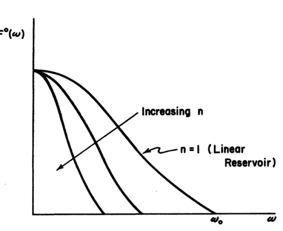
Figure III-5 demonstrates how the linear reservoir normalized amplitude spectrum has higher frequency components than Nash Models of order greater than 1 (which is the linear reservoir).

III-4.3 Selection of Response Function Duration

The time period for the system response was chosen arbitrarily to be that time which would allow 99% of the response to have occurred.

Again this was done by setting up an integral equation. As an example the linear reservoir formulation was used. The total area under the linear reservoir response curve is unity,so to find the time which should be used, the integrated system response for a linear reservoir was equated to .99, thus representing an area of 99%.

et/K = .99 III-16

OC

Figure III-5

Normalized Amplitude Spectrum Relationships for Nash Model

66

which is -t/K 1 -e -t/K =99 III-17 so T = -K-ln (.01) r III-18 = 4.605 K

Again, due to the difficulty of integrating some of the more complicated response functions, it was decided to use the linear

reservoir criteria with other linear models.

If this procedure were followed for the more complex system response models, it would be found that the integration increases in complexity. To alleviate this problem, the 'lag' of the complex

system responses was used in place of the lag for the linear reservoir response in Equation III-18. Although a large part of the area under the linear reservoir response curve is concentrated at the origin, this procedure provides a conservative but efficient solution for the response time period. The results of this procedure when applying a Nash Model response is found in Appendix B-1.

III-4.4 Selection of the Output Period

As mentioned in Section III-2.2 the selection of FOURT for calculating the Fourier transformations required choosing a time period representative of the output hydrograph. The response and input

added in order to extend these functions to the required time period. The algorithm utilized to do this is the following:

theory, is

so

The duration of the output, T , according to convolution the sum of the input duration, T_i, and response duration T_r

T = T. +T

o 1 r

where

III-19

T = the duration of the response to the system as given

r

in Section III-4.2

T. = the time of input duration.

1

Let Ni be the number of points in the input given at intervals Ati..

N.

=

i/At.

+ 1

1 1 III-20

Let N be the total number of points in the output which must be at the same interval, At., as the input, then

T N = - + 1

At.

1

= Ti/At.

_I

+ Tr/At. + 1 1 III-21 N. T i + r/At. 68

-Therefore the number of zeros to be added to the input function is given by:

Number of zeros = r/Ati III-22

1

The time period required for the input, response and output functions must be defined by the period Tr + Ti. Since the system responses will not be utilized in the time domain but only in the

forward transform, this procedure will transpose the time period into the number of input values as required by FOURT. For a further dis-cussion, refer to Section III-2.2.

III-4.5 An Example - The Theoretical Solution

Having solved the implementation problems, an example was tried. In order to have a basis for comparison, the theoretical solution of the example is obtained initially.

The example utilized was the response of a linear reser-voir to a square wave input of amplitude I and duration Ti.

The output function for this example can be found by convolution. The convolution integral for this example is:

_t t-T

f (t) = 1/K

j

I e K dT III-23

o o

This can be divided into two regions: tt f (t)= 1

J

I e

o

t-t

-

(-)

_{K_ dT For t T.} 1 III-24 = [I (1 - e )t and T. f (t) = 1 I 0

(t-T

I e K dT For t > T. o 1 III-25 T -t/K [e i / K -1] = I e[ T 0 i

The same result can be reached by finding the Fourier trans-form of the input and the response functions and multiplying them

together. The Fourier transform of the input is given by:

T. F () = 1 1 27 I o e dt = I 1 [e -j ] o 2 _ -jw III-26 o 70 -1

t-= I

-27 (jW)

(1- e -Ji0Ti)

The Fourier transform of the response function is defined

as: r co H (w) = 2T ( ) J 27T 0, 1 e K -t/K -jwt e dt III-27 1 1+jWK

The Fourier transform of the output function is obtained by multiplying these two results, i.e.

Fo () = Fi(W) H (w) 0 III-28 = I [j 1 (1 - e -WTi)

o

j -032K

21T

III-4.6 Obtained Results

A computer program was written to test the example discus-sed in Section III-4.5. The program udiscus-sed as input, the desired forcing

-function and the parameter, K, describing the linear reservoir model used. The program obtained the desired Nyquist frequency, , the corresponding time intervals at which the input must be given, At=r/o ,

and interpolated the input to the desired time interval if not given at that At. The program also evaluated the theoretical Fourier transform of the response function, found the transform of the input by using FOURT, multiplied them together, found the inverse of the resulting transform using FOURT to obtain the output function and finally plotted the resulting data together with the theoretical result. A copy of the program is included in Appendix A-1.

The program was tested with a square wave input having a maximum value of 3.0 and duration of 2 time units. The linear reser-voir model used a parameter K equal to 1.5. The plot of the resulting output function and its theoretical value can be seen in Figure III-6. As shown, the results are extremely accurate. The program with all the plotting, interpolating etc., took 2.67 seconds to execute on the

I.B.M. 360-67 computer system.

It is interesting to note that even though FOURT forward transforms showed marked aliasing effect (Figure III-4) and also failed to reproduce, exactly, the correct function when finding the inverse of a transform that was not its own (Figure III-3), that when the inverse of the forward transform is taken, after convolution,.resulted in such an accurate solution. This is due to the fact that the