Field observations of iceberg deterioration

(1)

Publisher’s version / Version de l'éditeur:

PERD/CHC Report, 2001-12

READ THESE TERMS AND CONDITIONS CAREFULLY BEFORE USING THIS WEBSITE.

https://nrc-publications.canada.ca/eng/copyright

Vous avez des questions? Nous pouvons vous aider. Pour communiquer directement avec un auteur, consultez la

première page de la revue dans laquelle son article a été publié afin de trouver ses coordonnées. Si vous n’arrivez pas à les repérer, communiquez avec nous à PublicationsArchive-ArchivesPublications@nrc-cnrc.gc.ca.

Questions? Contact the NRC Publications Archive team at

PublicationsArchive-ArchivesPublications@nrc-cnrc.gc.ca. If you wish to email the authors directly, please see the first page of the publication for their contact information.

NRC Publications Archive

Archives des publications du CNRC

For the publisher’s version, please access the DOI link below./ Pour consulter la version de l’éditeur, utilisez le lien DOI ci-dessous.

https://doi.org/10.4224/12340920

Access and use of this website and the material on it are subject to the Terms and Conditions set forth at

Field observations of iceberg deterioration

Veitch, Brian; Williams, Mary; Gardner, Alex; Liang, Bo

https://publications-cnrc.canada.ca/fra/droits

L’accès à ce site Web et l’utilisation de son contenu sont assujettis aux conditions présentées dans le site LISEZ CES CONDITIONS ATTENTIVEMENT AVANT D’UTILISER CE SITE WEB.

NRC Publications Record / Notice d'Archives des publications de CNRC:

https://nrc-publications.canada.ca/eng/view/object/?id=a1d4d7cc-c1d3-4975-b452-1affe1d91bf3 https://publications-cnrc.canada.ca/fra/voir/objet/?id=a1d4d7cc-c1d3-4975-b452-1affe1d91bf3

(2)

FIELD OBSERVATIONS OF

ICEBERG DETERIORATION

Prepared for

CHC, National Research Council

By

Brian Veitch, Mary Williams, Alex Gardner, Bo Liang Ocean Engineering Research Centre

Faculty of Engineering and Applied Science Memorial University of Newfoundland

St. John’s, NF, A1B 3X5, Canada

(3)

ABSTRACT

An investigation into iceberg evolution is reported. The main focus of the work was a unique field observation program in which photographs were taken of two grounded near shore icebergs over a period of several days each. In addition to the photographic observations of the above water portion of the icebergs, underwater sound recordings were made periodically. Sound records include a large cracking event in which the iceberg calved. The results of the field program are presented, including some specific local wave erosion data. This is part of an ongoing effort to understand the physical processes involved in iceberg evolution.

The work reported here was done under two separate contracts let to university based researchers: 391134 Iceberg Evolution Model - Wave Accelerated Erosion, and 391137 Iceberg Evolution Model – Field Observations. Both contracts dealt primarily with gathering field data, the former concentrating on visual information and the latter on acoustic data, so a common field program was mounted and the results are documented jointly.

(4)

TABLE OF CONTENTS

INTRODUCTION……….. 4

Background………. 4

Scope and Approach………... 5

FIELD OBSERVATIONS……….. 6

Instrumentation and Equipment……….. 6

Tors Cove……… 7

Little Harbour……….. 8

DISCUSSION AND CONCLUSIONS……….. 19

ACKNOWLEDGEMENTS……… 19

REFERENCES……… 20

APPENDIX A: Photographs of iceberg at Tors Cove

APPENDIX B: Photographs of iceberg at Little Harbour

APPENDIX C: Acoustic data of iceberg at Little Harbour

APPENDIX D: Tide tables

(5)

INTRODUCTION

Background

The annual flux of icebergs along the coast of Labrador and across the Grand Banks poses unique environmental challenges for exploration, production, and transport of hydrocarbon resources in the Newfoundland offshore area.

Icebergs pose risks to floating and fixed structures due to the potential impact loads. Subsea installations, such as pipelines, wellheads, flow lines, and risers are all exposed to iceberg risks in the form of scouring. These risks are amongst the most important drivers in oil and gas field development option selection, and have cost implications for development and operations on the order of $10s or $100s of millions per field. While these costs might not be eliminated, they may be reduced by developing better ways to manage the risks through increased knowledge.

The work reported here is part of a research program that aims to develop a model of iceberg evolution that follows the detailed shape changes due to continuous melting, discrete fragmentation, and reorientation due to stability considerations. The overall goal is to improve the knowledge of the evolution processes, which may lead to safer installations and lower costs.

A numerical model that can evaluate the orientation, floatation, and stability of an arbitrarily shaped iceberg was presented by Liang et al. (2001), based on a method outlined by Veitch & Daley (2000). The model integrates stability considerations and iceberg dynamics and incorporates shape changes due to simple melting processes. Modeling shape changes presents two main outstanding challenges. First, numerical modeling of complicated shapes and shape changes is technically and computationally demanding. Second, thermodynamic ablation processes for icebergs, specifically insolation, underwater convective melting, and wave accelerated melting have all been modeled with different degrees of sophistication, although field validation is relatively weak (e.g. Martin et al. 1977, White et al. 1980). The most significant of these is wave accelerated melting, which also has an important influence on calving fragmentation.

Wave erosion at the waterline of an iceberg produces protruding underwater rams and cantilevered shelves above water. The buoyancy forces on the former and the gravity forces on the latter frequently lead to large scale fractures of the iceberg. Removal of mass by a fracture changes the stability of the iceberg and exposes cold interior surfaces to warmer water, leading to further stresses and fractures. The resulting fragmentation reduces the mass of an iceberg at a much higher rate than wave erosion alone would achieve.

The sustained stress induced in the ice by the buoyancy and gravity forces induces accumulating viscoelastic strain due to grain boundary sliding, and microcracking occurs at a critical level of the viscoelastic strain (Sinha 1982). Damage due to microcracking is progressive, and eventually a global fracture is precipitated. The stresses estimated in Diemand et al. (1987) due to the buoyant forces on a protruding underwater ram are sufficient to cause cracking in freshwater ice at -5° in approximately 30 minutes; the time is reduced at higher temperatures (Sinha 1984). Thus although fracture appears catastrophic, cracking activity is continuous.

A measurement of the level of cracking activity would provide information on the rate of invisible deterioration of the iceberg. High frequency acoustic emissions can be used to monitor the evolution of microcrack damage in ice at laboratory scale (Sinha 1996). Large scale fractures in ice are low frequency acoustic sources which propagate strongly through the water in the

(6)

horizontal direction (Farmer & Xie 1989). For these reasons, we undertook an investigation of the feasibility of acoustic measurements of iceberg cracking activity.

According to available information, there have been only two previous investigations of iceberg noise. The first concluded that iceberg noise was equivalent to white noise (Urick 1971). In the second, a rise in spectrum noise density between 5 and 50 kHz in the vicinity of an iceberg was attributed to the release of air bubbles during melting. It appears that there have been no previous investigations of the concept of acoustic signals due to cracking activity.

Scope and Approach

The current work deals specifically with wave accelerated thermodynamic erosion and fragmentation. The main component of the work was a field observation program. The results of the field work can be used to develop and validate wave erosion, calving and possibly other models.

The aims of the program were to make relatively long term visual observations of iceberg deterioration, particularly at the air-water-ice interface where thermal erosion is accelerated due to wave action, and to collect acoustic data from icebergs, particularly cracking noise.

As financial resources for the project were relatively modest, the only practical means of gathering field data was from shore. Only grounded near shore icebergs provide the conditions to make the necessary observations for sufficient durations.

(7)

FIELD OBSERVATIONS

Instrumentation and Equipment

The field program consisted of long term observations of two near shore grounded icebergs. The first was a small iceberg grounded in Tors Cove (47°14′N, 52°51′W) on the east coast of the Avalon Peninsula, about 40 kilometers south of St. John’s. Its deterioration was followed for a period of 7 days, from May 9th to May 15th, at which point it was abandoned in favour of a larger target. The second iceberg was grounded in the Main Tickle (49°38′N, 54°41′W) just east of Little Harbour, near Twillingate on South Twillingate Island, in Notre Dame Bay. It was observed for 6 days, from May 27 to June 1. After the first week in June, no more suitable icebergs were found grounded in accessible near shore locations.

In selecting photographic instrumentation, resolution, data storage, and cost were considered. The Sony DSC-S70 digital camera, which records high quality images on memory sticks, was selected. At maximum optical zoom, the image size/focal length ratio is 0.343, and the maximum resolution image is 2048×1536 pixels. Using the larger image dimension, this gives an image resolution of 0.084m at 500m distance. Two DSC-S70 units were procured, for backup and to permit simultaneous recording of different views. In the field, the cameras were installed in weatherproof housings on fixed tripods.

In addition, a personal Sony DCR-TRV330 digital 8 video camera was used to make continuous recordings of the iceberg so that any fragmentation and reorientation events might be captured. In fact, two significant fragmentation events at the Little Harbour iceberg were captured on video tape. A theodolite was used to survey the field sites and local iceberg geometry, but was unfortunately damaged at the start of the work in Little Harbour and was consequently not used there.

In selecting acoustic instrumentation, frequency band, signal levels, noise levels, data acquisition, and cost were considered. Available information indicates that there will be acoustic signals from an iceberg at high frequencies due to microcracking and bubbles. The frequency of signals due to large cracks may be estimated in two ways. The basic response frequency, f, is approximately

v

f = /2L (1)

where v is the crack velocity and L is the crack length (Haykin et al. 1994). For simple cracks, the mean velocity is approximately 50m⋅s-1

(Gagnon et al. 1999). Hence for a crack length of 0.5m, the base frequency would be approximately 50Hz. For the second estimate, consider that the signal transmitted to the water will be strongest at wavelengths on the order of twice the diameter of the iceberg (Crocker 1998). For a 60m diameter berg, using a sound speed of 3780m⋅s-1

in ice, the strongest response would be at 63Hz. Both of these estimates indicate that there could be acoustic information from the iceberg down to 50Hz. On the other hand, the stick-slip nature of the cracking may reduce the effective crack length in equation (1) to several grain diameters. Hence generated frequencies could be as high as 5kHz. On these considerations, the frequency range 25Hz to 10kHz was selected for observation.

In the ocean, ambient noise is present across the spectrum. Shipping noise is strongest between 102 and 103 Hz. At high frequencies, there is noise generated by wind and waves (Zedel

(8)

et al. 1999). Hence it can be anticipated that separating signals from ambient noise will be difficult. As there is no prior information on measurements of this nature, estimating signal levels is difficult. The approach taken to deal with both signal and noise was to deploy the instrument as close to the sound source as practical and safe, and to make the signal level on site adjustable.

Hydrophones normally used in oceanographic research cost between $500 and $20,000, and the data acquisition systems are cumbersome and very expensive. The present project called for an inexpensive package that could be manually deployed. The instrument selected is a commercially available omnidirectional piezo hydrophone, the DolphinEAR. The frequency response is a few Hz to more than 22kHz, and the sensor is packaged with power supply and cable. Two DolphinEAR units were procured, for redundancy.

Data was collected and stored at the surface on a Sony MZ-R700, a consumer portable minidisc recorder with an extended recording mode that allows 4 hours of data to be recorded onto a single removable disc. The Sony MZ-R700 kHz bandwidth is given as 0 to 20 kHz. In the analysis phase of the project, it was discovered that the extended recording mode compromises bandwidth, and the actual data bandwidth was only 10kHz. At the time of the field program, the Sony MZ-R700 was not available in Canada at retail. Due to price and restricted availability, only one unit was procured. A backup recording system, a professional quality analogue tape recorder with a 60 minute capacity, was on hand but not required.

The hydrophone was suspended from a buoyant watertight box which contained the minidisc. Signal levels were adjusted by the operator on site. The system could be easily carried by one person, and deployed manually from an open boat. The disc capacity limited a deployment to 4 hours, but since the field team was on site, this did not constitute a significant problem.

Tors Cove

A small iceberg was spotted on May 8th at Tors Cove. It was approximately 50 meters long and was rather too far offshore to make the planned photographic observations. Furthermore, the site was not conducive to deploying the hydrophones due to the distance that the iceberg was offshore and the direct exposure of the coast to ocean waves. As there was no other known near shore iceberg targets at this date, a decision was made to use this small iceberg as the subject of shakedown tests for the equipment and the field crew. A convenient position to set up the camera equipment on the coast was found. Further, the proximity of Tors Cove to St. John’s meant that the 2 man field team could commute to the site daily. The field crew consisted of a co-op engineering student and an engineering graduate student – the third and fourth authors of this report.

The iceberg, which is shown in Figure 1, was already smoothed by water action when the observations began, indicating that the above water portion had likely been previously immersed. Two waterline notches can also be seen. One is partially exposed – on the left side in the picture – due to a recent reorientation of about 10° to the waterline position shown. Another reorientation prior to that, also about 10°, has exposed the notch that is approximately parallel to the current waterline. The patrol boat in the foreground gives some sense of scale. Several of the photos taken at Tors Cove are presented in Appendix A.

(9)

Figure 1. Small iceberg at Tors Cove, May 9, 2001.

Little Harbour

Following the trial observations made at Tors Cove, a second target was sought. Ice charts indicated the presence of near shore icebergs scattered along the coast from the Strait of Belle Isle, along to White Bay and Note Dame Bay, and beyond to Fogo. Site visits along the coast from May 21 to 24 confirmed some of these targets and more. Several candidate icebergs were identified from amongst this group, including one in Little Harbour. In the two days it took to mobilize the field equipment and return to the north coast, almost all of the candidate icebergs had moved offshore. The mobility of the icebergs made the ice charts of only marginal help in planning the detailed field program.

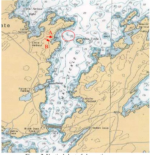
The site ultimately selected is shown on the navigation chart in Figure 2 and in the aerial photograph reproduced in Figure 3. In both figures, the arrows indicate the positions of the cameras and the ellipse encompasses the location of the iceberg. The iceberg, which is shown in Figure 4 and in the frontispiece, was approximately 125×106

kg. It was not grounded all of the time and sometimes drifted within the circumscribed area. The local bathymetry was ideal for the field program in that it confined the iceberg to a very small area even though it was not firmly grounded and was sometimes free to drift. Further, the water depth increased rapidly from the beach to 20m and 30m. This made the relatively long term observations of a medium sized iceberg possible from vantage point only about 500m away.

Logistically, the site was also favourable. The two man field team was accommodated at a local B&B in Little Harbour and could walk from the village to the site along a foot path. A camp was set up in a field just off the beach. Gear was stored in the tent to protect it from the weather. Likewise, the tent provided a refuge for the field team from inclement weather.

(10)

The data sampling protocol and the sampling equipment were simple. Two still cameras were set up on tripods at the top of the beach. Plastic housings were mounted over the cameras to protect them from the elements. Their locations were separated by a rocky headland and some light brush. The setup made a planned evaluation of the utility of stereo photography impractical to pursue. However, the visual observations that were made were adequate for studying the effects of wave erosion. Stereo photos would be of limited added value in this regard.

Still digital photographs were taken approximately every 30 minutes from both camera locations, provided the iceberg was visible. Occasionally, the iceberg drifted to a position that, from the perspective of one of the cameras, put it behind the headland. Images were recorded on memory sticks throughout the day and then backed up to a laptop every evening. The video camera, which was also mounted on a tripod, recorded to high quality digital 8 tape. Changes in water depth due to tides were not discernible at the field site, although tide tables for Twillingate are given in Appendix D, for the record.

A B

Figure 2. Nautical chart of observation area

(Reproduced from chart 4863: Bacalhao Island to Black Island, Canadian Hydrographic Service).

The hydrophones were hung from a floating water tight aluminum box which housed the sound recording equipment. The hydrophone box unit was deployed and retrieved daily from a boat. In the mornings, two local men picked up the field team in a small boat and motored near

(11)

the iceberg. The hydrophone box was launched over the side along with a small anchor, which provided its mooring. In the evening, the hydrophone box was retrieved in the same manner. The field crew were also able to take additional photographs and video from the vantage point of the small boat, which included the parts of the iceberg not visible from shore.

The weather conditions were mixed during the field program, as can be seen in Table 1 along with some general daily notes about the iceberg. Similarly, Table 2 reports a daily record of the water temperature, and the number of photographs taken from both shore locations and from the daily boat trip around the iceberg. It also indicates the extent of the hydrophone data. In all, almost 400 photos were taken, along with about 17 hours of underwater acoustic recordings. The photographic records are presented in Appendix B and the hydrophone data are presented in Appendix C.

The results span a relatively long time period – 6 days – as planned. Further, the extent of the photographs, coupled with the acoustic and video recordings that include a number of major fragmentation events, combine to make the results unique.

Figure 3. Aerial photograph chart of observation area

(Reproduced from A-18633-221, Air Photo Division, Energy Mines & Resources)

For most of the time, there was no discernible change in the iceberg’s above water shape from hour to hour. Even changes from day to day due to above water surface melting were not discernible. Significant shape changes were due to fragmentation and wave erosion, which appeared to be intimately connected in the cases observed. Several fragmentation events were captured on video tape, along with before and after photographs.

(12)

An example of a large fragmentation event is shown in the video stills on the left hand side of Figure 4. A large part of the ice pinnacle on the right hand of the iceberg collapsed. Consequently, that side of the iceberg rose out of the water and the left side became more immersed. Although it is not shown in this sequence, a second fragmentation event occurred at about the time that the iceberg reached its maximum roll angle (the last picture in the Figure 4): much of the ice above water on the left hand side then collapsed. Note that the underwater shape of the iceberg shown on the right hand side is conjecture.

Table 1. Daily log: weather conditions and notes for Little Harbour iceberg.

weather Notes

24-May-01 overcast all day, 6°C No significant iceberg activity

27-May-01 clear w/ occasional cloud, 6°C No significant iceberg activity; theodolite damaged 28-May-01 clear, 18.6°C, light SE winds No significant iceberg activity

29-May-01

clear in am, 21.2°C; clouding over w/

occasional rain in pm, 24.7°C Iceberg fragmented & foundered, captured by video and hydrophone 30-May-01 rain, occasionally heavy, 13.3-17.3°C Small fragmentation event, captured by hydrophone

31-May-01

rain in am, clearing around noon, 14.1°C, SE wind; warming in pm, 18.3-18.5°C, wind shifting to S with light mist

Iceberg fragmented & foundering, captured by video, not hydrophone

01-Jun-01

Sunny, occasional fog rolled, 9.1–

11.3°C No significant iceberg activity Table 2. Daily log: water temperature and data coverage of Little Harbour iceberg.

water temp. # photos, camera A # photos, camera B # photos,

boat hydrophone data

[°C] [-] [-] [-] [-]

24-May-01 9 9 0 not deployed 27-May-01 3.9-4.0 25 15 35 5 hours

28-May-01 3.3 31 20 19 cable broken - no data

29-May-01 7.1 35 27 19

5 hours, including major fragmentation event

30-May-01 3.9-7.3 35 23 17

5 hours, including minor fragmentation event

31-May-01 6.3 27 10 17

2.5 hours, excluding significant fragmentation event

01-Jun-01 7.4 14 5 0 not deployed

(13)

Figure 4. LHS: Video stills of fragmentation. RHS: Corresponding simulation results.

(14)

These pictures illustrate that the numerical model developed by Liang et al. (2001) is capable of simulating this and other iceberg stability and motion phenomena. But the main point in the present context is that, in terms of the observed changes over a period of days, it was only the fragmentation events that were easy to capture in detail, and then only with the combination of video and still photograph records.

The second phenomenon that caused observable changes in the iceberg’s shape was wave erosion. As these changes occurred primarily underwater, they were difficult to record on a regular basis, particularly when the wave environment was relatively benign. Collecting data on wave erosion was made more difficult by the iceberg’s mobility. That is, the iceberg sometimes yawed slowly over a period of minutes to hours so that the portions visible to the still cameras changed. It was possible to piece together a progression of wave erosion using the daily video records taken from the boat to complement the still photographs.

Also, the iceberg deteriorated significantly over the observation period, with commensurate changes to its orientation and floatation position. There were two consequences to this. First, it meant that the time span over which wave erosion at a particular location could be observed was limited due to reorientation and repositioning of the iceberg. On the other hand, major movements also revealed portions of the iceberg that were previously submerged. The result is that the observations of wave erosion were more difficult than anticipated, particularly given the ideal field site. On the other hand, the pictures include evidence of wave erosion, but the evidence has to be pieced together. Further the fact that the iceberg was deteriorating during the observation period adds to the potential value of the data for additional information, such as on fragmentation.

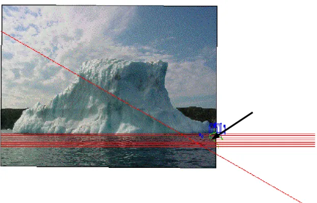
The sequence of pictures in Figures 5 to 8 illustrates a sample of wave erosion data. Figure 5 shows the end result. The profile at right corresponds to a particular surface of the iceberg prior to its being exposed to wave erosion. This original surface is shown by crude white line in Figure 6. The profile to the left in Figure 5 shows the profile at the same part of the iceberg after it had been exposed to wave erosion. Figure 7 shows the same iceberg as in Figure 6, but after it had moved to a new orientation where the new waterline intersected with the original surface. With reference to Figure 7, the location of interest – where the wave erosion is occurring - is at the extreme right hand side. Only the above water part of the local surface profile can be seen. It is only after another change in orientation, shown in Figure 8, that the underwater part of the wave eroded surface becomes visible and allows it to be recorded. Pulling data from the photo record is a laborious process. The erosion represented in the figures took place over a period of 47¼ hours, from 17:35 May 27 to 16:50 on May 29.

(15)

Original surface profile Eroded surface profile

Figure 5. Outline profiles of the iceberg showing wave erosion.

Figure 6. The surface that eventually gets eroded by waves is indicated by an arrow.

(16)

Figure 7. The original surface (see Figure 6) is now at the waterline at the extreme right.

Figure 8. After a second reorientation the eroded surface is visible.

(17)

The acoustic data system functioned satisfactorily. It was deployed 5 times between May 27 to 31. On May 28, the hydrophone was damaged during launch. The unit was replaced with the backup, but the electrical connections were not completed correctly and no data were collected. The major fracture event of May 29 was recorded on the hydrophone, as was a small fracture event on May 30. A second major fracture on May 31 occurred after the minidisc was full; the event is not in the data set, but the signals leading up to it are.

The acoustic data records, trimmed to remove the portions contaminated by the deployment vessel, are contained on four CD-ROMs, submitted with this report (copies available from the CHC/NRC). Appendix C is a listing of the CD-ROM contents.

In the field, the acoustic data were checked by listening to playback from the minidisc. No further analysis was attempted. In the laboratory, the data were examined using a standard PC soundcard and commercial sound analysis software, Cool Edit 2000. Two factors reduced the quality of the data collected. First, the recorded audio is highly distorted. The likely cause is overload of the recorder input by the output of the hydrophone. The second factor, not clear in the recorder specifications, is that the long play mode is accomplished by sampling alternately on each channel. The sampling rate of 22 kHz results in a bandwidth of 11 kHz on one channel.

Figure 9 shows the spectrum of typical a sample of the hydrophone data. The horizontal axis is time in minutes, the vertical axis is frequency, and the intensity indicates energy level. There is no significant energy above 11 kHz, which is half of the standard 22 kHz sampling rate. There is a strong band of energy at approximately 2800 Hz that is consistent across all the data. The consistency of the energy band makes it seem unlikely that this is a part of the underwater acoustic environment, although 3 kHz does correspond to typical wave noise energy. Other possible sources are the compression process or the input distortion.

1:00

Figure 9. Spectrum of untreated hydrophone data.

(18)

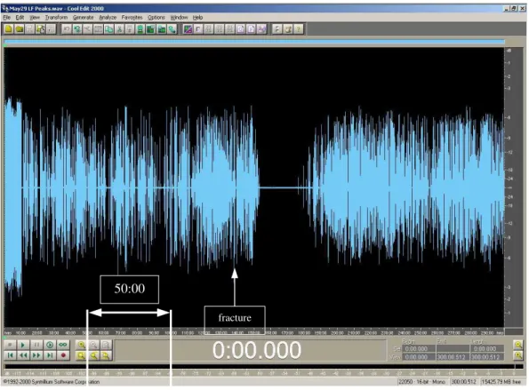
Samples of the data were filtered experimentally in an effort to isolate useful information. Samples representing the iceberg at rest and the fracture events were both considered. Distinct information appeared to emerge at low frequencies. Hence a specific effort to isolate low frequency peaks was undertaken. A frequency selective expansion process, with the gain for peaks above -10dB set to negative infinity, was applied to the data below 300 Hz. This resulted in a data file with the low frequency peaks of interest completely removed. Subtracting this from the original data produced a file containing only the low frequency peaks. Figure 10 is the result for a 300 minute portion of the May 29 record. The fracture event occurs at approximately 140 minutes into the record. Figure 11 is a time expansion, with the fracture at approximately 4:30 minutes.

50:00

fracture

Figure 10. Low frequency peaks in May 29 data. The major fracture occurs at 140 minutes.

From the frequency estimates made above (Instrumentation and Equipment), crack propagation is a plausible explanation for the low frequency peaks, though not the only one. The expanded record in Figure 11 shows that the peaks are distinct, spasmodic, and highly clustered near the main event. The longer record shows a dropout following the major event. This could be a cessation of fracture activity due to stress relief in the fracture. An alternate explanation is that the peaks are due to the iceberg grinding on the bottom, and the gap is a result of the berg lifting off the bottom following mass reduction.

The acoustic data have not been examined in a systematic manner. It is possible that other combinations of threshold, peak length, and frequency will reveal other features. It is likely, though not conclusively proven, that information about crack development and iceberg state of deterioration is contained in the acoustic signals. It is not yet possible to draw conclusions about the extent and quality of the information.

(19)

1:00

Figure 11. Expanded time scale of fracture portion of Figure 10. The major fracture event is at approximately 4:30 minutes.

(20)

DISCUSSION AND CONCLUSION

The field observations of an iceberg reported here include above water photographic (and video) information spanning 6 days, and long sequences of acoustic records. The data is unique and has potential value for predictive modeling, whether to help build a model or validate one. In particular, the data on wave erosion and on calving due to wave erosion, which the field program set out to collect, were captured over a long time and included several significant fragmentation events.

When planning a field program that depends on the co-operation of icebergs, flexibility is crucial. The iceberg that grounded in Little Harbour presented an ideal opportunity to meet the field program’s aims. Indeed, the proximity of the iceberg to shore, its lengthy stay in the same location, its advanced stage of decay and corresponding liveliness, and its convenient location meant that the data collected exceeded expectations. As a consequence, more effort went into preserving and reporting the data, rather than on analyzing a small subset of the results. The example of wave erosion at the iceberg’s waterline given above illustrated that, while there is a lot of potentially valuable information in the data, getting it out is laborious.

The work also demonstrated the feasibility of monitoring iceberg condition by acoustic means. The method of collecting the data was adequate for the purpose of testing the feasibility. Significant improvements in the quality of the data may be achieved using the same instrumentation. The bandwidth can be increased to 22 kHz by avoiding the extended recording mode, and the distortion can be reduced by matching hydrophone output and recorder input levels. Likely noise sources in the current data are grinding of the iceberg on the bottom, and wave action on the nearby shoreline. It is likely that data from a freely floating iceberg, distant from the shore, would have significantly less background noise.

A scientific instrument grade hydrophone would have greater dynamic range and a calibrated response over its measurement frequency band. Although these factors were not limitations in the present work, an upgrade is recommended for future investigations.

The results of the current work have potential application in two directions. First, for the scientific work of iceberg deterioration studies, acoustics may provide useful data on fracture activity and rate of deterioration. Second, the pattern of fracture activity may provide a warning sign of impending catastrophic failure.

ACKNOWLEDGEMENTS

The field program that made up the main component of this work was run by Alex Gardner, a co-op engineering student from Memorial University, who spent the summer working on this project. The second member of the field team was Bo Liang, a Master of Engineering student at Memorial, who helped out during the field work. Both did an excellent job and their contribution to the success of the work is acknowledged with gratitude.

The authors also thank Dr. Garry Timco, who acted as project manager on behalf of the Canadian Hydraulics Center, National Research Council.

(21)

REFERENCES

Crocker, M. J., Ed. 1998. Handbook of Acoustics, Wiley.

Diemand, D., Nixon, W. A., and Lever, J. H. 1987. On the splitting of icebergs - natural and induced. Proceedings, Offshore Mechanics and Arctic Engineering, ASME, pp.379-385. Farmer, D. M. and Xie, Y. 1989. The sound generated by propagating cracks in sea ice. Journal

Acoustical Society of America, 85(4): 1489-1500.

Gagnon, R. E., Williams, F. M., and Sinha, N. K. 1999. High speed video observations of fracture from beam bending experiments on sea ice. Proceedings, Port and Ocean

Engineering Under Arctic Conditions, pp.25-36.

Haykin, S. S., Lewis, E. O., Raney, R. K. (eds.) 1994. Remote sensing of sea ice and icebergs. Wiley Series in Remote Sensing, John Wiley.

Liang, B., Veitch, B., and Daley, C. 2001. Iceberg deterioration and stability. Proceedings, Port

and Ocean Engineering under Arctic Conditions, Vol.2, pp.1007-1016.

Martin, S., Josberger, E., and Kauffman,P. 1977. Wave-induced heat transfer to an iceberg. In Josberger, E.G. 1977. A laboratory and field study of iceberg deterioration. Proceedings

Iceberg Utilization, A.A.Husseiny (ed.), Pergamon Press, pp.245-264.

Sinha, N. K. 1982. Delayed elastic strain criterion for first cracks in ice. Proceedings, IUTAM

Conference on Deformation and Failure of Granular Materials, IUTAM, pp.323-330.

Sinha, N. K. 1984. Intercrystalline cracking, grain boundary sliding, and delayed elasticity at high temperatures. Journal of Materials Science, 19: 359-376.

Sinha, N. K. 1996. Creep cracking and acoustic emissions in polar shelf ice at high temperature of 0.96 Tm. Proceedings,14th World Conference on Non Destructive Testing, Vol.4, pp.2475-2478.

Urick, R.S. 1971. The noise of melting icebergs. Journal Acoustical Society of America, 50(1, pt. 2): 337-341.

Veitch, B., and Daley, C. 2000. Iceberg evolution modeling. OERC-2000-02, Ocean Engineering Research Centre, Memorial University of Newfoundland, for National Research Council of Canada, PERD/CHC Report 20-53, 49 pp.

White, F.M., Spaulding, M.L., and Gominho, L. 1980. Theoretical estimates of the various mechanisms involved in iceberg deterioration in the open ocean environment. CG-D-62-80, University of Rhode Island for United States Coast Guard, 126 pp.

Zedel, L., L. Gordon and S. Osterhus. 1999. Ocean ambient sound instrument system: acoustic estimation of wind speed and direction from a sub-surface package. Journal of Atmospheric

and Oceanic Technology, 16: 1118-1126

(22)

APPENDIX A: Photographs of iceberg at Tors Cove

Iceberg on May 10, with close up (from video camera still).

Iceberg on May 12, with close up (from video camera still).

(23)

APPENDIX B: Photographs of iceberg at Little Harbour Note: Copies of the photographic data on CD can requested of the CHC/NRC.

(24)

360-4

27, 360-1 27,

27, 360-3 27,

(25)

27, 360-5 27, 360-6

(26)

27, 360-9 27, 360-10

(27)

27, 360-13 27, 360-14

(28)

27, 360-17 27, 360-18

(29)

360-22

27, 360-21 27,

(30)

360-28

27, 360-25 27,

27, 360-27 27,

(31)

27, 360-29 27, 360-30

(32)

360-34

(33)

360-4

28, 360-1 28,

28, 360-3 28,

(34)

360-8

28, 360-5 28,

28, 360-7 28,

(35)

360-12

28, 360-9 28,

28, 360-11 28,

(36)

360-14

28, 360-13 28,

(37)

28, 360-17 28, 360-18

(38)

360-2

29, 360-1 29,

(39)

29, 360-5 29,

29, 360-7 29,

360-6

(40)

360-10

29, 360-9 29,

(41)

29, 360-13 29,

29, 360-15 29,

360-14

(42)

29, 360-17 29, 360-18

(43)

30, 360-1 30, 360-2

(44)

360-6

30, 360-5 30,

(45)

360-10

30, 360-9 30,

(46)

30, 360-13 30, 360-14

(47)

(48)

360-4

31, 360-1 31,

31, 360-3 31,

(49)

360-8

31, 360-5 31,

31, 360-7 31,

(50)

360-12

31, 360-9 31,

31, 360-11 31,

(51)

31, 360-13 31,

31, 360-15 31,

360-14

(52)

31, 360-17 31, 360-17

(53)

28, 17:01 29, 10:01

(54)

29, 11:32 29, 11:55

(55)

29, 12:53 29, 12:53

(56)

29, 14:00 29, 14:00

(57)

29, 15:02 29, 15:02

(58)

30, 10:37 30, 10:37

(59)

30, 11:31 30, 11:32

(60)

30, 12:35 30, 13:35

(61)

30, 13:33 30, 13:33

(62)

30, 14:32 30, 14:32

(63)

30, 15:32

(64)

31, 11:18 31, 12:01

(65)

31, 13:28 31, 14:01

(66)

31, 15:32 31, 16:02

(67)

1, 11:20 1, 11:45

(68)

24, 13:15 24, 13:50

(69)

15:49

24, 15:18 24,

(70)

27, 10:32 27, 11:10

(71)

27, 12:44 27, 12:45

27, 13:14 27,

27, 12:44 27, 12:45

(72)

27, 13:44 27, 13:44

(73)

27, 14:46 27, 14:46

(74)

15:44

27, 15:44 27,

(75)

27, 16:45 27, 16:45

(76)

28, 11:33 28, 11:33

(77)

28, 12:32 28, 12:32

(78)

28, 13:29 28, 13:29

(79)

28, 14:34 28, 14:34

(80)

28, 15:30 28, 15:30

(81)

28, 16:27 28, 16:27

(82)

28, 21:00 28, 21:00

(83)

29, 10:42 29, 10:42

(84)

29, 11:29 29, 11:30

(85)

12:33

29, 12:19 29,

(86)

13:59

29, 13:32 29,

(87)

14:31

29, 14:31 29,

(88)

15:01

29, 15:01 29,

(89)

29, 15:30 30, 10:36

(90)

11:07

30, 11:07 30,

(91)

30, 11:30 30, 11:30

(92)