HAL Id: inria-00419952
https://hal.inria.fr/inria-00419952
Submitted on 25 Sep 2009HAL is a multi-disciplinary open access
archive for the deposit and dissemination of sci-entific research documents, whether they are pub-lished or not. The documents may come from teaching and research institutions in France or
L’archive ouverte pluridisciplinaire HAL, est destinée au dépôt et à la diffusion de documents scientifiques de niveau recherche, publiés ou non, émanant des établissements d’enseignement et de recherche français ou étrangers, des laboratoires
Landscape regularity modelling for environmental
challenges in agriculture
El Ghali Lazrak, Jean-Francois Mari, Benoît Marc
To cite this version:
El Ghali Lazrak, Jean-Francois Mari, Benoît Marc. Landscape regularity modelling for environmental challenges in agriculture. Landscape Ecology, Springer Verlag, 2009, Landscape Ecology, 25 (2), pp.169-183. �10.1007/s10980-009-9399-8�. �inria-00419952�
Landscape regularity modelling for environmental
challenges in agriculture
El Ghali Lazrak∗ Jean-Fran¸cois Mari † Marc Benoˆıt ‡
Abstract In agricultural landscapes, methods to identify and describe meaningful landscape patterns play an important role to understand the in-teraction between landscape organization and ecological processes. We pro-pose an innovative stochastic modelling method of agricultural landscape organization where the temporal regularities in land-use are first identified through recognized Land-Use Successions (LUS) before locating these suc-cessions in landscapes. These time-space regularities within landscapes are extracted using a new data mining method based on Hidden Markov Mo-dels. We applied this methodological proposal to the Niort Plain (West of France). We built a temporo-spatial analysis for this case study through spa-tially explicit analysis of Land Use Succession (LUS) dynamics. Implications and perspectives of such an approach, which links together the temporal and the spatial dimensions of the agricultural organization, are discussed by as-sessing the relationship between the agricultural landscape patterns defined using this approach and ecological data through an illustrative example of bird nests.
Keywords Cropping system • Land-Use Changes • Temporo-spatial analysis • Data mining • Hidden Markov Model (HMM) • Hierarchical Hid-den Markov Model (HHMM) • Landscape Agronomy • Agricultural patterns • Landscape Ecology • Poitou-Charentes (France)
The original publication is available at www.springerlink.com, Landscape Ecology Modelling, DOI 10.1007/s10980-009-9399-8
∗INRA, UR 055, SAD ASTER, 662, avenue Louis Buffet F-88500 Mirecourt, France
email: [email protected] (Corresponding author)
†UMR-CNRS 7503 LORIA, B.P. 239, F-54506 Vandœuvre-l`es-Nancy, France e-mail:
‡INRA, UR 055, SAD ASTER, 662, avenue Louis Buffet F-88500 Mirecourt, France
1
Introduction
Agroecosystems are the major mode of land-use both at French (52%) and European (42%) levels. Since 1962, under the influence of the Common Agricultural Policy, agricultural production has intensified and its effects on biodiversity are no longer a matter of debate (Donald et al. 2001 ; Robin-son and Sutherland 2002). Biodiversity conservation and restoration have become a social necessity and a political goal. Yet the practical means to achieve them in agroecosystems are still to be developed (Turner 2005 ; But-ler et al. 2007). To understand the interaction between landscape organiza-tion and ecological processes, one needs to identify and quantify landscape patterns in meaningful ways (Turner 1990).
In agricultural landscapes, land-uses are heterogeneously distributed among different polygons (agricultural parcels). They also display dynamic patterns as a result of crop cycles, agricultural practices and other driving forces of land-use changes.
Recent studies (R´etho et al. 2008) have investigated the relationship of restricted areas of agricultural landscape with the diversity of animal species. On wider areas the complexity of agricultural landscapes needs to be simplified before investigating the relationships between a set of land-scape indices (predictor variables) and ecological variables. This complexity of agricultural landscapes is generally simplified by using coarse agricultu-ral land-use classes (e.g. Poudevigne and Alard 1997 ; Donald et al. 2001 ; Fuller et al. 2005). In this paper, we introduce a method which takes into account greater agricultural knowledge to identify and describe agricultural patterns. This description of agricultural patterns could improve the assess-ment of biodiversity in agricultural ecosystems at small geographical scales, and the assessment of water resource degradation in agricultural regions (Mignolet et al. 2007).
Agricultural biodiversity is related to soil, climate and cropping system interactions (Forman and Godron 1986). We focused on the factors managed and driven by farmers. For us, they correspond to cropping systems, which were categorized by Sebillotte (1974) into two components : (i) crop succes-sions, seen as the ordered sequences of soil occupancy in each field and (ii) technical sequences, defined as the ordered sequences of cultural practices on a crop for production.
This research falls within the realm of landscape agronomy, the aim of which is to study the organization of farming activities on small geographical scales (Benoˆıt et al. 2007). Its scope is at the conjunction where technical farming activities in the fields, the influence of EU and world regulations
impact on agriculture. We now see an increasing attention being given to local issues as result of farming activities and environmental preservation in particular. Landscape agronomy as an emerging discipline combines the concepts and methods of both (i) geographers and (ii) agronomists (Benoˆıt and Papy 1997), by respectively combining the following :
1. multi-scale modelling for land-use changes and for the investigation into territorial consistencies (Velkamp and fresco 1997 ; De Loning et al. 1999) ; and
2. analytical methods to describe the reasoning behind the way regio-nal agricultural systems work. These methods notably rely on the construction and then on the spatialization of farming classifications (Perrot 1990 ; Landais 1996 ; Mignolet and Benoˆıt 2001 ; Leisz et al. 2005 ; Mignolet et al. 2007).
The way a farmer organizes his territory is a time and spatial process. The land-use category of a given site depends upon the land-use categories of the neighbourhood. For example, grasslands are mainly located in areas close to villages, whereas maize fields are usually far away from forests. The Markov Random Field (MRF) is an elegant mathematical model to take into account the uncertainty of locations in the vicinity of a given place. This model clusters the territory into patches where the distribution of land-use categories follows a certain probability law. On the other hand, the land-use category at time t (the current year is the usually admitted time slot unit) for a field depends also upon its former category at time t − 1, t − 2, etc. Since the late nineteenth century, plant successions have been studied on vegetation dynamics of natural ecosystems as reviewed by Glenn-Lewin and van der Maarel (1992). Among several approaches for studying vegeta-tion dynamics, statistical models, especially Markov models, have already proved their usefulness (Usher 1992 ; Castellazzi et al. 2008). However, the precision of Markov models depends upon the quality of parameter estima-tion (Peet et al. 1992). The parameters of first-order Markov models can be tuned with the help of experts (Castellazzi et al. 2008). They can also be automatically estimated by means of algorithms such as the Baum-Welch algorithm (Welch 2003) when dealing with Hidden Markov Models (HMMs). In addition, compared to a first-order HMM, a higher-order HMM can ade-quately assign a probability to longer successions of land-use categories and reveal some temporal patterns.
In this paper, we propose a unified Markovian framework to : 1. represent both spatial and temporal dependencies in sites, and ;
2. cluster a territory into patches where the successions of land-use cate-gories are drawn by a higher-order Markov process.
Our main objective is to develop a generic method aimed at describing agricultural landscapes through cropping system patterns. As Moonen and Bˆrberi (2008) emphasize the importance of territorial organization as a determinant of functional biodiversity, two applications of these patterns are :
1. to help understand environmental and natural processes in crop re-gions in Europe in relation with the organization and dynamics of agricultural landscapes, and ;
2. to develop a knowledge of agricultural dynamics, which may facilitate political decision-making and forecasting.
After presenting the characteristics of the landscape we studied, we will give a brief theoretical background of our research procedure. Then, we ex-plain this procedure in two stages. The first stage aims at modelling the diversity of the cropping systems, independently from their location within the landscape. The second stage is focused on the localization of these crop-ping systems that have been revealed in the previous stage. We propose to build a temporospatial analysis through spatial analysis of crops dynamics. This approach links together the temporal and the spatial dimensions of the agricultural organization. Its implications and perspectives are discussed in an illustrative example drawn from the Niort Plain by assessing the rela-tionship between the agricultural landscape patterns and the distribution of Montagu’s Harrier nests.
2
Methods
2.1 Study area
We apply our landscape regularity modelling method on one grain-growing area in France : the Niort Plain situated within the plain of NiortBrioux, south of DeuxS`evres in Poitou-Charentes region (46.2 N, 0.4 W).
Since 1994, the Chiz´e Centre for Biological Studies (CNRS1
unit) has been conducting a research program on the impact of farm management strategies on biodiversity in grain growing plains. This program focuses on the NiortBrioux plain (350 km2
). It examines the contribution of grasslands to the conservation of various species of birds in a way compatible with an
1
economically viable farming activity. Since the beginning of this research program, the surveyed zone has been progressively enlarged : 20 km2
in 1994, 200 km2
in 1995, 320 km2
in 1996 with a relative stabilization until 2005 followed by other enlargements to 420 km2
in 2006 and to 430 km2
in 2007. In this paper, we consider the period of 12 successive years starting in 1996.
2.2 The long-term land-use survey
In the framework of its biodiversity research program in relation with agricultural practices, the Chiz´e Centre for Biological Studies (CEBC2
) car-ries out, every year, two land-use surveys (in April and June). These two yearly surveys take into account both early harvested and late planted crops. In each survey, the occupancy of parcels is noted down distinguishing 47 uses (42 agricultural uses, 3 urban uses and 2 forest land-uses) as detailed in Table 1. Each parcel contains one type of crop and its physical boundaries can be a river, a path or a field limit. Each year, sur-veyors also update the parcel limits when a change is observed. The changing limits of the agricultural parcels led to the definition of elementary parcels, which resulted from a spatial union of previously updated parcel limits. The study area contains 19,000 elementary parcels, covering an area of 430 km2
. The collected data is stored in a GIS geodatabase, in vector format.
2.3 Theoretical background
2.3.1 Markov random fields and Hidden Markov Models
Temporal and (or) spatial process can be spontaneously represented by stochastic graphs. The nodes are associated to some random variables (X, Y ). The Xs take their values from a finite set of classes
Ω = { ω1, ω2, . . . , ωk}
called the labels. The Y s take their values from the input data – also called the observations – of the process at a specific time slot or space location. The transitions represent the temporal or spatial dependencies between the nodes. The interest of such models is to compute the a posteriori probability P(X1 = x1, X2 = x2, . . . , Xn= xn | Y1= y1, Y2 = y2, . . . , Yn= yn) for
a given configuration of labels (x1, x2, . . . , xn) drawn from Ω and a set of
observations (y1, y2, . . . , yn) in order to measure how the configuration fits
2
the model assuming the observations. In a particular family of stochastic graphs – aka Markov Random Fields (MRF), the probability of observing Xi = xi assuming the values on all the other nodes depends on a limited set
of nodes called the neighbouring nodes of Xi
P(Xi= xi|X1 = x1, . . . , Xj6=i= xj, . . . , Xn= xn)
= P (Xi = xi|{ Xneighbour of i= xi} )
In this paper, we present our work using second-order Hidden Markov Models (HMM2) to approximate MRF. We rely on the assumption that the distribution of land-use categories in an area at time t – the blocking plan – depends on the blocking plan observed at time t − 1 or t − 2 according to the order of the model (first-order or second-order). Hidden Markov Models analyze one dimensional sequences of observations. They differ from Markov chains (Castellazzi et al. 2008) through the presence of a supplementary hid-den layer of nodes that models the structure of the data. This hidhid-den layer is a second-order Markov chain that governs the sequence of random variables capturing the variability of the observations. Hidden Markov Models have been successfully introduced in 1976 in speech recognition (Jelinek 1976), image processing (Benmiloud and Pieczynski 1995), biology (Hughey and Krogh 1996), and ecology (Le Ber et al. 2006). They can be used adequately to model temporal and spatial stochastic processes.
In order to model MRFs, Benmiloud and Pieczinski (1995) have pro-posed a method to convert a spatial representation of the data into a one dimensional sequence by means of a fractal curve – the Hilbert Peano curve – that spans the two dimensional space. Two points that are close to one another on the curve are close in the plane. The opposite is not true. Despite this drawback, they show that the classical HMM training algorithms give performances comparable to the more complicated algorithms involved in Markov Random Fields.
2.3.2 HMM2 definitions An HMM2 is defined by :
– A set S = { s1, s2, . . . , sN} of N states that are the outcomes of the
variables Xt , where t = 1, . . . , T
– A transition matrix A = (aijk) over S 3
, where aijk is the a priori
transition probability P (Xt= sk|Xt−2 = si, Xt−1 = sj) for the
hid-den Markov chain to be in state skat index t assuming it was in state
sj at index t − 1 and si at index t − 2 . The Markov assumption states
– A set of N discrete distributions : bi(.) is the distribution of
observa-tions associated with state si. This distribution may be parametric,
non parametric or even given by a HMM in a hierarchical HMM. 2.3.3 HMM2 properties
The second-order Hidden Markov Models are based on the probability and statistics theories. They implement an unsupervised training algorithm – the Baum-Welch algorithm – that estimates the HMM2 parameters from a corpus of observations. The estimated model enables to segment each sequence in stationary and transient parts and to build up a classification together with its a posteriori probability
P(X = conf iguration | Y = observations ) .
In a first-order HMM, the probability that a sequence of n observations – called the state duration probability – is captured by state i follows a geo-metric decay defined by (aii)n, where aii is the a priori probability of the
loop over state i. In a second-order HMM, the state duration is governed by two parameters, i.e. the probability of entering a state only once, and the probability of visiting a state at least twice, with the latter modelled as a geometric decay. This distribution better fits a probability density of dura-tions than the exponential distribution of a first-order HMM. This property is of great interest when a HMM2 models a process in which a state captures only one or two observations (Mari et al. 1997).
Furthermore, the very success of HMMs is their robustness. Even when the input data do not fit a given HMM, it can give interesting results by discovering spatial and temporal regularities.
2.3.4 Hierarchical HMM (HHMM)
We model the spatial structure of the landscape by a MRF whose sites are random land-use sequences. These sequences are modelled by a temporal HMM2. This leads to the definition of a hierarchical HMM where a master HMM2 approximates the MRF. Then, the probability of a temporal land-use sequence is given by a temporal HMM2 as fully described by Fine et al. (1998) and Mari and Le Ber (2006). This hierarchical HMM is used to segment a landscape into regions. The temporal evolutions of the regional sites are land-use sequences that are modelled by a temporal HMM2. The use of hierarchical HMM in data mining is a special case of stochastic models as described by Le Ber et al. (2006) and may be summarized as the following steps :
1. Specify the topology of a hierarchical HMM ; 2. Gather spatio-temporal data ;
3. Train the HMM on these data using the Baum-Welch algorithm ; 4. Segment the data and interpret the content of the classes ; 5. Design a new model and go back to step 1.
2.3.5 ArpentAge : a data mining Software ArpentAge3
(Analyse de R´egularit´es dans les Paysages : Environne-ment, Territoires, Agronomie = Landscape Regularities Analysis : Environ-ment, Territories and Agronomy) is an acronym that also means landscape surveying in French. It is the name of our knowledge discovery system based on higher-order hidden Markov models for analyzing spatio-temporal data bases. It takes as input an array of discrete data – the rows represent the spatial sites, the columns represent the time slots – and clusters the terri-tory into patches whose crop sequences are extracted. This software allows the user to specify the architecture of the Markov model according to his objectives and the data. Displaying tools and the generation of shape files have also been implemented. The results of ArpentAge are interpreted and validated by domain specialists (i.e. agronomists).
2.4 A computer limitation issue when dealing with huge amount of data
Using a Hilbert-Peano fractal curve requires regularly spaced input data points. This is why we rasterized land-use data by following a systematic and regular sampling pattern (10 m x 10 m). Data were then formatted so that the rows represent the spatial sites (sampled points) and the columns the time slots of attributes. A huge corpus with around 8 million rows has been obtained. However, the estimation of HMM2’s parameters is a memory consuming process that can saturate even large computer memories. In order to help reduce the requirement of the memory resources, we choose to control two factors : (i) the length of the elementary LUS, and (ii) the size of the corpus of observations through the sampling resolution.
3
3
Results
3.1 Preliminaries : scaling the method to deal with huge amounts of data
3.1.1 Choice of the succession length
The length of Land-Use Successions (LUS) influences the interpretabi-lity of the final model. The longer the succession is, the more useful it is for agronomists. However, the total number of LUS is a power function of these succession lengths. Memory resources required during the estimation of HMM2 parameters increase with large numbers of LUS.
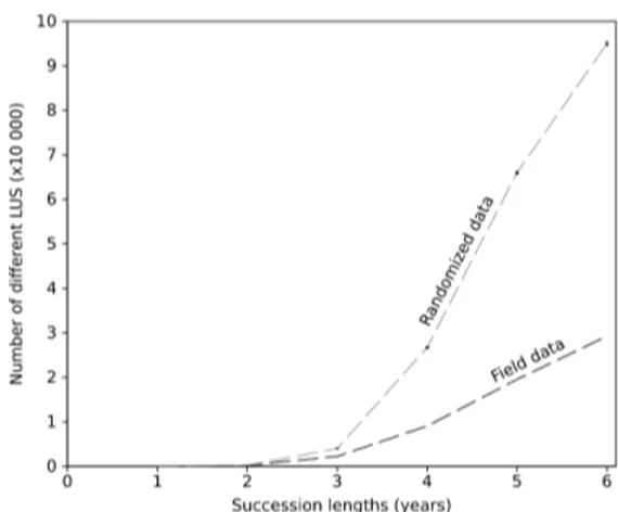
To help decide on the succession length, we compared the diversity of LUS between field-collected data and randomly generated data for different lengths of successions (Figure 1). In the Niort Plain case, we can see that a 4-year succession length begins to differentiate from the random case. This reinforced our choice of the quadrennial succession as the elementary observation symbol in modelling the Niort Plain case study. Further down in this paper, the 4-year LUS will be sometimes referred to as quadruplets.
Fig. 1 – Compared diversity of LUS between field-collected data and 10 random generated data sets for different succession lengths
3.1.2 Choice of the spatial resolution
At regional scales, high-resolution samplings generate large amounts of data. With such amounts of input data, only rough models can be tested.
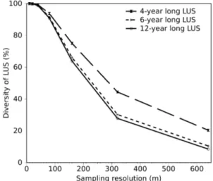
On the other hand, with coarse resolution samplings, small parcels are omit-ted. In order to have an objective criterion for choosing the optimal spatial resolution, information loss in terms of LUS diversity was estimated for in-creasingly coarse resolution samplings. Figure 2 shows curves for the three considered LUS lengths that follow quite similar trends. As a compromise, we chose the (80 m x 80 m) resolution that led to a corpus 64 times smaller than the original one, with only a loss of 6% in information diversity.
Fig. 2 – Information loss in terms of LUS diversity in relation to sampling resolutions for three succession lengths. Tested resolutions are : 10, 20, 40, 80, 160, 320 and 640 m. Irregularity in sampling intervals is dictated by an algorithmic constraint, the resolution must be proportional to a power of 2. The most precise resolution is considered as the reference (100%)
3.2 Modelling the diversity of farming activity within land-scapes
The approaches to model the diversity of farming activities differ accor-ding to whether one is considering the production system or the cropping system. Numerous classification models represent the diversity of agricultu-ral production systems in a given region, the choice of which depends signi-ficantly on the time and space scales investigated. On the other hand, few models have been developed to represent the diversity of cropping systems on a regional scale. Here we propose an approach to model this diversity by
first dealing with the Land-Use Successions (LUS) and then their locations. 3.2.1 The model representing the location of the diversity of LUS The aim is to identify temporal stabilities in Land-Use Successions, and to locate them in landscapes. The first step was to build a typology of ho-mogeneous land-use categories (Table 1). Then, we identified the successions in our landscape (Table 2). The third step identified the dynamics of LUS (Table 3 and Figure 3). The fourth step identified patches of LUS (Figure 4 and Figure 5).
3.2.2 Land-use typology
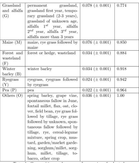
In this first step we identified the major land-uses and classified them into homogeneous categories. Based on an arbitrarily frequency defined thre-shold (0.01 i.e. 1% of a given land-use among the total number of all land-use records in the data set), the land-use types were differentiated into major (>0.01) and minor (<0.01) land-uses. Then, major land-uses were grouped with other similar major or minor land-uses to form homogeneous land-use categories (hereafter called “main land-use categories”). Finally, the remai-ning minor land-uses were grouped into a residual category called “Others”. This last land-use category is rather heterogeneous and will not be conside-red as a main land-use category in the following. Table 1 shows the result of this classification. Land-use category Land-use Frequency (Confidence, P=0.05) Cumulative frequency Wheat (W)
wheat, bearded wheat, ce-real 4
0.337 0.337
Sunflower (S)
sunflower, ryegrass followed by sunflower
0.139 0.476
Rapeseed (R)
rapeseed 0.124 (± 0.001) 0.600 Urban (U) built area, peri-village, road 0.096 (± 0.001) 0.696
4
Cereal is used when the species can not be identified by the surveyor (it can be wheat, barley, ryegrass or other)
Grassland and alfalfa (G)
permanent grassland, grassland first year, tempo-rary grassland (2-3 years), grassland of unknown age, alfalfa 1st year, alfalfa
2nd year, alfalfa 3rd year,
alfalfa more than 3 years
0.078 (± 0.001) 0.774
Maize (M) maize, rye grass followed by maize
0.076 (± 0.001) 0.850 Forest and
wasteland (F)
forest or hedge, wasteland 0.034 (± 0.001) 0.884
Winter barley (B)
winter barley 0.034 (± 0.001) 0.918 Ryegrass
(Y)
ryegrass, ryegrass followed by ryegrass
0.024 (± 0.001) 0.942
Pea (P) pea 0.022 (± 0.001) 0.964
Others (O) spring barley, grape vine, spontaneous fallow in June, foxtail millet, flax, oat, clo-ver, field bean, rye grass fol-lowed by tillage, rye grass followed by unknown, spon-taneous fallow followed by tillage, rye, cereal-legume mixture, spring crop, mus-tard, garden/market garde-ning, sorghum/millet, sorg-hum, millet, tillage, to-bacco, other crop
0.036 (± 0.001) 1.00
Tab. 1: Composition and average frequencies of adopted land-use categories. The “Frequency” refers to the average for the total area covered by all land-uses of a given land-use category. This average was computed over a 12 year period
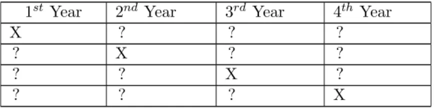
3.2.3 The conceptual model representing the diversity of LUS Using 4-year long LUS to model the Niort Plain landscape required the reduction of the large number of these successions (many thousands, see Figure 1). Most of the time, in the study period, the 10 main land-use categories almost describe the whole area of the Niort Plain (over 96%, see Table 1). On this basis, we chose to represent the diversity of LUS in as many classes as there are main land-use categories. Table 2 represents the search pattern used to extract all the successions involving a given main land-use category. For each main land-use category X, we look for the list S(X) of quadruplets in which X was involved.
1stYear 2nd Year 3rd Year 4th Year
X ? ? ?
? X ? ?
? ? X ?
? ? ? X
Tab.2: Search pattern for extracting all 4-year long LUS in-volving one of the main land-use categories. X represents the current main land-use category, and ? any land-use category
Actually, Wheat (W), Sunflower (S) and Rapeseed (R) are generally integrated in a same succession (such as S-W-R-W, S-W-S-W, R-W-R-W, S-W-W-W, R-W-W-W, etc.). So, making a common class of these three crops allowed better results. To deal with this case, the above notation can be generalized to : S(X,Y,...) to denote the class of successions that involve at least one of the main land-use categories X, Y, etc.
We listed the resulting classes of successions as quadruplets “of interest” that we quantified by their frequency in the data corpus. The large num-ber of quadruplets can then be reduced by using an appropriate threshold of cumulative frequency or by choosing a given number of most frequent quadruplets.
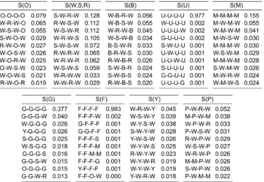
3.2.4 The LUS temporal dynamics analysis by means of HMM2 Table 3 shows the results of the temporal data mining analysis perfor-med by the search patterns described in Table 2. Table 3 summarizes the distribution of quadruplets within the resulting classes of LUS.
Classes S(U) and S(F) are stable classes, they are mainly represented by only one quadruplet : U-U-U-U and F-F-F-F respectively.
Tab. 3 – Results of the temporal analysis for the Niort Plain case study over the 1996-2007 period : frequency distribution of LUS for each class of successions
S(W,S,R) is the most dominant class. Its quadruplet distribution allows the deduction of principal rotations such as : (i) “S-W-R-W” which is a quadrennial rotation composed of the four circular permutations of quadruplets : S-W-R-W, R-W-S-W, W-S-W-R, W-R-W-S. Its fre-quency is around 40% ; and (ii) ”S-W” and ”R-W” : which are two biennial rotations deduced from the quadruplets : S-W-S-W, W-S-W-S and R-W-R-W, W-R-W-R respectively. Their frequencies are slightly over 10%. These three rotations represent around 60% of the total composition of the S(W,S,R) class.
S(B), S(M), S(G), S(Y) and S(P) are less ordered classes and some-how reflect the farmers’ ”freedom” as to their land allocation with the corresponding categories of crops (namely winter Barley (B), Maize (M), Grassland and alfalfa (G), rYegrass (Y) and Pea (P)). This cor-roborates our choice in considering the succession classes –S(X) – as the regularities to be located in the next step, rather than considering rotations.
S(M) : In this class, the quadruplet distribution allows to deduce 3 main regularities : (i) 15% of the maize monoculture shown by the M-M-M-M quadruplet, and (ii) about 10% of the biennial rotation WM deduced from the quadruplets M-W-M-W and W-M-W-M, and (iii) about 0.8% of the quadrennial rotation “M-W-S-W”.
S(P) : In this class, the quadruplet distribution shows the quadrennial rotations “PWRW” and ”PWSW” whose respective frequencies are roughly 10%.
S(B) : In class, the quadruplets distribution shows two triennial rotations ”RWB” and ”SWB” whose respective frequencies are around 10%. S(O) : In this class, the O-O-O-O LUS characterizes the parcels covered
by vineyards or market-garden crops that, mainly, keep the same land cover during all the study period. Other quadruplets incorporating a O appear with lower frequencies and reflect that this land cover can appear randomly in numerous parcels. The mean blocking plan of the O occupation is roughly 3 % over the 12 year study period. Therefore O occupations disappear in the amount of W, S, R in these parcels because the O occupations are not integrated in some specific rotations. This leads to a distribution’s estimation almost equal to the S(W,S,R) distribution. We found this result by computing the divergence between these two distributions and found them close to each other.
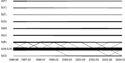
Fig.3 – Results of the temporal analysis for the Niort Plain case study over the 1996-2007 period : Markov diagram shows the temporal dynamics of LUS classes after 50 iterations of the EM algorithm. The x-axis represents the study period divided into sub periods of 4 years. The y-axis represents the classes of LUS involving : Wheat (W), Sunflower (S), Rapeseed (R), Urban (U), Maize (M), Grassland and alfalfa (G), Forest and wasteland (F), winter Barley (B), rYegrass (Y), and Pea (P). Others (O) is a residual land-use category that contains successions of less frequent land-use types. Diagonal transitions stand for inter-annual changes. Horizontal transitions indicate inter-annual stability. Only transitions whose frequencies are greater than 0.01 are displayed. The line width reflects the a posteriori probability of the transition assuming the observation of the 12-year LUS.
Figure 3 shows the dynamics of the resulting classes of LUS in the Markov diagram. The quite constant width of horizontal lines of the Markov diagram indicates that during the whole study period (1996-2007), no major change has affected the dynamics of LUS. This figure shows diagonal transition lines between S(B) and S(W,S,R) classes and between S(O) and S(W,S,R). In the Niort area, Barley is cultivated in 3-year rotations (”RWB” or ”SWB”). When these 3 year rotations are over, the farmers can start new rotations spanning 2 years (”RW”, ”SW”) or 4 years (”SBRW”). The 3-year rotations are related to the horizontal lines in the S(B) class whereas transitions from a 3-year rotation to a 2- or 4-year rotation trigger a diagonal line to the S(W,S,R) class.
The diagonal transitions between S(O) and S(W,S,R) are explained by the closeness of the two distributions.
3.2.5 The LUS spatial analysis by means of HHMM2
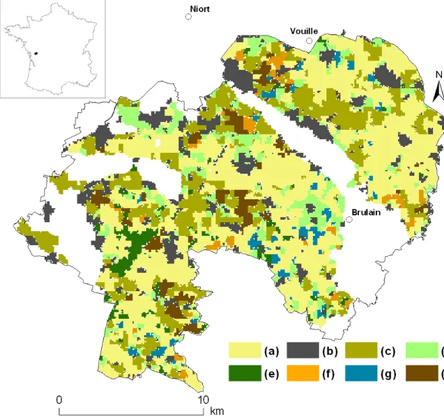
In this step, temporal regularities (i.e. classes of successions) found in the temporal analysis step were localized within the Niort Plain landscape. As we observed that LUS was stationary over the 1996-2007 period, we used a simple temporal HMM2 to represent the states of the hierarchical HMM2. This temporal model does not segment the study period but rather consi-ders it as a whole. This model has 2 states. One describes the distribution of the quadruplets of interest related to the class S(X), the other state cap-tures the distribution of the quadruplets in the neighbourhood. The Markov field introduces a blur in the patch’s frontier and in the patch estimation because a site is classified not only based on its temporal characteristics (the quadruplet succession) but depends now on the classification of the neigh-bouring sites. The map of the Niort Plain shown in Figure 4, is the result of the temporo-spatial Markov modelling process that defines a classifica-tion based on the LUS that have been observed between 1996 and 2007. The landscape is seen as patches of LUS. For each class of patches, there is a corresponding distribution of LUS, which is summarized in a diagram format (Figure 5).
The spatial partitioning with the HHMM2 fails to locate the S(O) class within the Niort Plain landscape. The spatial analysis located two small patches covering only 0.05 % of the classified area, which correspond to six elementary parcels. For visibility and significance considerations, we did not represent the corresponding patches in the resulting map.
The class of patches labelled (a) represents the S(W,S,R) class of LUS in almost 70% of the total area. In the remaining area there are residual
Fig. 4 – The Niort Plain landscape as patches of LUS. White areas in the map are unclassified because they were insufficiently surveyed over the 1996-2007 period. Location of the Niort Plain in France is depicted in the upper left-hand box. The map legend is given in Fig. 5
Fig. 5 – Distribution of the most frequent LUS for each class of patches shown in Figure 4. Each diagram plots separately the distribution of searched successions (lower rectangle) and residual successions (upper rectangle). The residual successions result from both smoothing patches and border effects introduced by the Markov field. Bold quadruplets belong to the successions of interest and italic quadruplets are residual successions. The frequency of each quadruplet has been computed by dividing the count of the quadruplet by the size of the class
successions i.e. successions that contain neither Wheat nor Sunflower nor Rapeseed.
The class of patches labelled (b) represents successions in the Urban category. In this class of patches, the Urban category is present in LUS in more than 60% of the total area. The blur introduced by the Markov field can be seen in this patch. The temporal analysis exhibited a 0.975 probability for the quadruplet U-U-U-U, the Markov field lowers this probability to 0.60. The residual part is mainly populated by the quadruplets of the S(G) class that are typical of urban neighbourhoods. The same influence can be seen in the S(G) class where U-U-U-U is found in the residual part.
The map unit (c) represents the S(M) class of LUS in almost 60% of the total area, where around 10% has been cultivated with maize monoculture for at least 4 years (the quadruplet M-M-M-M).
The map unit (d) represents the S(G) class of LUS in almost 50% of the total area. It is mainly composed of old pastures (20% of G-G-G-G quadruplets), but also more recently converted to Grassland category areas (Y-G-G-G, W-G-G-G). Cropping systems using Wheat, Rapeseed and Sunflower are more likely to be found around grasslands.
The map unit (e) refers to Forest and Wasteland category in 70% of the total area of the associated patches. The only F-F-F-F quadruplet showing that Forests and Wastelands are rather stable represents this category. Close to forests, one is likely to find Grasslands, Urban areas and some cropping systems including Wheat, Rapeseed and Sunflower as shown in the residual part.
Map units (f,g,h) are less well classified. This is shown by their large resi-dual intervals due to the neighbourhood effects. However, the corresponding patches are particularly interesting because they contain crops (respecti-vely winter Barley (B), rYegrass (Y) and Pea (P)) whose frequency is more important than elsewhere.
4
Discussion
4.1 A new framework for Landscape regularity modelling : a Time x Space analysis
The main stream of our research on landscape regularities modelling consists in a Time x Space analysis based on a stochastic approach. We pointed out the consistency of crop sequences (Le Ber et al. 2006 ; Castel-lazzi et al. 2008) by a LUS temporal analysis before locating the temporal regularities in the landscape by means of HHMM2.
The main advantages of this method are :
1. to be related with the farmers’ choices since they use crop sequences instead of using a crop by crop organization,
2. to improve the landscape analysis with respect to field uses, and 3. to automatically learn the model parameters from the observation
data.
In this paper, we described a new data mining method that processes a huge corpus of land-use observation data from a medium-size territory in order to :
1. choose the succession length of land-use, 2. choose the spatial resolution,
3. define a conceptual model for representing the diversity of LUS, 4. and finally, create maps that show patches of temporal regularities.
These maps give an objective classification of the territory based on its pluriannual agronomic organization. They are of great interest when the ecological process under study and the spatial organization of the patches are correlated.
4.2 The need of perennial information systems
We used a data base built on a long term survey led by a CNRS team that involves a huge amount of human labour.
Another source of land-use maps is satellite remote sensing images, whose spatial and temporal resolutions have been greatly improved in recent years. As a common tool in Geography, it can be used to map land-uses on a regional scale (Girard et al. 1990 ; Veldkamp and Lambin 2001 ; Verburg and Veldkamp 2001). We put forward the hypothesis that our modelling method can handle those remote sensing data if they are able to inform a long time period with a sub-annual resolution.
4.3 Linking with biodiversity resources
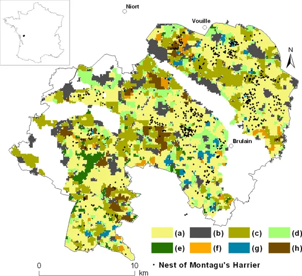
To illustrate an attempt at linking agricultural patterns at a regional scale and ecological data, we chose a heritage species of birds : Montagu’s Harrier. Nest locations of Montagu’s Harrier overlapped the patches of LUS as depicted in Figure 6.
The joint representation of nest locations and landscape organization is useful for ecologists to formulate research issues and hypotheses related to
Fig. 6 – Spatial distribution of Montagu’s Harrier nests (Circus pygargus) within patches of LUS. The nests belong to the 1996-2007 period, which is the same period used to define patches of LUS. The location of nests results from a comprehensive monitoring throughout the study area each year from late April to late July
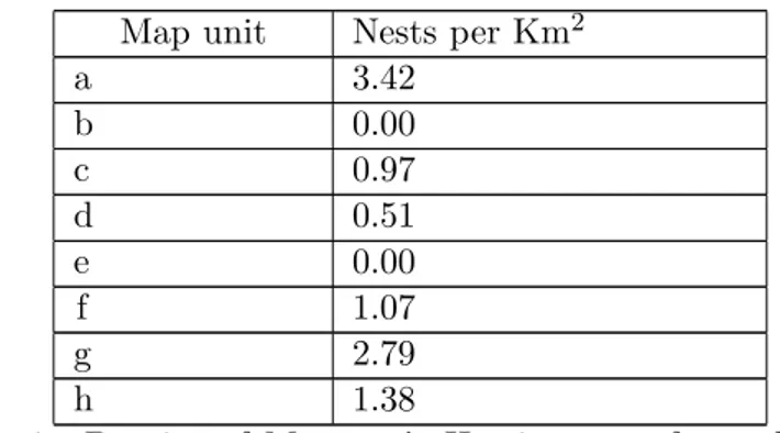
Map unit Nests per Km2 a 3.42 b 0.00 c 0.97 d 0.51 e 0.00 f 1.07 g 2.79 h 1.38
Tab. 4: Density of Montagu’s Harrier nests for each map unit. The nests belong to the 1996-2007 period
this bird’s distribution over the agricultural area and over a longer period than one year. For instance, one can see that while patches of class (a) are homogeneously distributed over the studied area, one can wonder why the number of nests in the South-West patches of this class is so low compared to the mean density. Ornithologists make the assumption that the presence of egg predators in the forest (patch e) prevent Montagu’s Harriers from nesting in the vicinity and leads them to adopt a semi colonial behaviour. But this statistical curiosity is still an open issue.
This illustration provides only broad tendencies on the joint relationship between Montagu’s Harrier and its surrounding landscape. In fact, involved territories in the Montagu’s Harrier’s life are substantially larger than the nesting scale (Salamolard 1997). Landscape units have to be linked with animal territories and habitats. Future works will be to evaluate the areas involved in the definition of animal territories. Ecological and agricultural pattern interactions could be more deeply explored by following an organism-centered view of landscape heterogeneity (Turner 2005). This can be achie-ved by coupling agricultural and ecological data in the data mining process in order to extract joint regularities of both agricultural landscape descrip-tors and ecological indicadescrip-tors. Indeed, this needs a close collaboration with ecologists. This is what we intend to investigate in our future research work.
4.4 Contribution of agronomy to environmental issues at regional scales : contribution of Landscape Agronomy to Landscape Ecology
From an agronomist’s point of view, we consider that agricultural land-scapes are created by farmer practices (Morlon and Benoˆıt 1990 ; Le Ber and Benoˆıt 1998), and we seek to describe and to model the driving forces of landscape changes. In the present work, we hope to contribute to Land-scape Agronomy which is an emerging field (Benoˆıt et al. 2007) that holds three main scientific tasks :
1. to identify the rules and laws within the landscape that link environ-mental processes and farming systems ;
2. to build scenarios for partners showing the implications of land-use practices for landscapes, and ;
3. to build bridges between agronomists, geographers and ecologists on a common scientific field of interest : landscape.
As a contribution to Landscape Ecology, Landscape Agronomy is inten-ded to give the ”managing dimension” to the eco-field hypothesis of Farina and Belgrano (2006).
5
Acknowledgments
This work was supported by the ANR-ADD-COPT project, the API-ECOGER project and the ANR-BiodivAgrim project. We thank the CNRS team in Chiz´e for their data records obtained from their ”Niort Plain data base”. We thank Anne Mimet and the anonymous reviewers for their useful comments.
6
References
Benmiloud B, Pieczynski W (1995) Estimation des param`etres dans les chaˆınes de Markov cach´es et segmentation d’images. Traitement du signal 12 :433-454
Benoˆıt M, Mignolet C, Herrmann S et al (2007) Landscape as designed by farming systems : a challenge for landscape agronomists in Europe. In : Far-ming Systems Design 2007, Methodologies for Integrated Analysis of Farm Production Systems, Catania, 10-12 September 2007
Benoˆıt M, Papy F (1997) Pratiques Agricoles et qualit´e de l’eau sur le territoire alimentant un captage. In : Neveu A, Riou C, Bonhomme R et al (eds) L’eau dans l’espace rural (Production v´eg´etale et qualit´e de l’eau). Aupelf-Uref-UREF & Inra ´editions, Paris, pp 323-338
Butler SJ, Vickery JA, Norris K (2007) Farmland biodiversity and the footprint of agriculture. Science 315 :381-384
Castellazzi M, Wood G, Burgess P et al (2008) A systematic represen-tation of crop rorepresen-tations. Agricultural Systems 97 :26-33
De Koning GHJ, Verburg PH, Veldkamp A et al (1999) Multi-scale mo-delling of land use change dynamics in Ecuador. Agricultural Systems 61 :77-93
Donald PF, Green RE, Heath MF (2001) Agricultural intensification and the collapse of Europe’s farmland bird populations. Proceedings of the Royal Society of London 268 : 25-29
Fine S, Singer Y, Tishby N (1998) The Hierarchical Hidden Markov Model : Analysis and Applications. Machine Learning 32 :41-62
Forman RTT, Godron M (1986) Landscape ecology. John Wiley, New York
Fuller RM, Devereux BJ, Gillings S, Amable GS, Hill RA (2005) Indices of bird-habitat preference from field surveys of birds and remote sensing of land cover : a study of south-eastern England with wider implications for conservation and biodiversity assessment. Global Ecology and Biogeography 14 :223-240
Girard CM, Benoˆıt M, De Vaubernier E et al (1990) SPOT HRV data to discriminate grassland quality. International Journal of Remote Sensing 11 :2253-2267
Glenn-Lewin DC, van der Maarel E (1992) Patterns and processes of vegetation dynamics. In : Peet RK, Glenn-Lewin DC, veblen TT (eds) Plant Succession : Theory and Prediction. Chapman & Hall, London, pp 11-44
Hughey R, Krogh A (1996) Hidden Markov Models for Sequence Ana-lysis : Extension and AnaAna-lysis of the Basic Method. Computer Applications in the Biosciences 12 :95-107
Jelinek F (1976) Continuous speech recognition by statistical methods. Proceedings of the IEEE 64 :532-556
Lambin E, Geist H, Lepers E (2003) Dynamics of land-use and land-cover change in tropical regions. Annual Review of Environment and Resources 28 :205-241
Landais E (1996) Typologies d’exploitations agricoles. Nouvelles ques-tions, nouvelles m´ethodes. Economie Rurale (SFER) 236 :3-15
Le Ber F, Benoˆıt M (1998) Modelling the spatial organisation of land use in a farming territory. Example of a village in the Plateau lorrain. Agronomie 18 :103-115
Le Ber F, Benoˆıt M, Schott C et al (2006) Studying crop sequences with CarrotAge, a HMM-based data mining software. Ecological Modelling 191 :170-185
Leisz SJ, Thu Ha N, Bich Yen N et al (2005) Developing a methodo-logy for identifying, mapping and potentially monitoring the distribution of general farming system types in Vietnam’s northern mountain region. Agricultural Systems 85 :340-363
Mari J-F, Le Ber F (2006) Temporal and spatial data mining with second-order hidden markov models. Soft Computing 10 :406-414
Mari, J-F, Haton, J-P, Kriouile, A (1997) Automatic word recognition based on second-order Hidden Markov Models. IEEE Transactions on speech and Audio Processing 5 :22-25
Mignolet C, Benoˆıt M (2001) R´eflexions sur une segmentation r´egionale selon la diversit´e des syst`emes techniques agricoles - Cas de la plaine des Vosges. G´eomatique 11 :177-190
Mignolet C, Schott C, Benoˆıt M (2007) Spatial dynamics of farming practices in the Seine basin : Methods for agronomic approaches on a regional scale. Science of the Total Environment 375 :13-32
Moonen A-C, Bˆrberi P (2008) Functionnal biodiversity : An agroecosys-tem approach. Agriculture, Ecosysagroecosys-tems and Environment 127 :7-21 Morlon P, Benoˆıt M (1990) f tude m´ethodologique d’un parcellaire d’exploitation agricole en tant que syst`eme. Agronomie 6 :499-508
Peet RK, Glenn-Lewin DC, Veblen TT (1992) Plant Succession : Theory and Prediction. Chapman & Hall
Perrot C (1990) Typologie d’exploitations construite par agr´egation au-tour de pTM
les d´efinis ˆ dire d’experts. Proposition m´ethodologique et pre-miers r´esultats obtenus en Haute-Marne. Prod Anim 3 :51-66
Poudevigne I, Alard D (1997) Landscape and agricultural patterns in rural areas : a case study in the Brionne Basin, Normandy, France. Journal of Environmental Management 50 : 335-349
Reboul C (1976) Mode de production et syst`emes de culture et d’´elevage. Economie Rurale 112 :55-65
Retho B, Gaucherel C, Inchausti P et al (2008) Spatially explicit popu-lation dynamics of Pterostichus Melanarius I11. (Coleoptera : Carabidae) in response to changes in the composition and configuration of agricultural landscapes. Landscape and Urban Planning 84 :191-199
Robinson RA, Sutherland WJ (2002) Post-war changes in arable farming and biodiversity in Great Britain. Journal of Applied Ecology 39 :157-176
Salamolard M (1997) Utilisation de l’espace par le Busard cendr´e Circus pygargus. Superficie et distribution des zones de chasse. Alauda 65 :307-320 Sebillotte M (1974) Agronomie et agriculture. Essai d’analyse des tˆaches de l’agronome. Cahiers de l’ORSTOM 24 :3-25
Turner MG (1990) Spatial and temporal analysis of landscape pattern. Landscape Ecology 4 : 21-30
Turner MG (2005) Landscape ecology : what is the state of the science ? Annual Review of Ecology, Evolution, and Systematics 36 :319-344
Usher MB (1992) Statistical models of succession. In : Peet RK, Glenn-Lewin DC, veblen TT (eds) Plant Succession : Theory and Prediction. Chap-man & Hall, London, pp 215-246
Veldkamp A, Fresco LO (1997) Reconstructing land use drivers and their spatial scale dependence for Costa Rica (1973 and 1984). Agricultural Sys-tems 55 :19-43
Veldkamp A, Lambin E (2001) Predicting land-use change. Agriculture, Ecosystems and Environment 85 :1-6
Verburg PH, Veldkamp A (2001) The role of spatially explicit models in land-use change research : a case study for cropping patterns in China. Agriculture, Ecosystems and Environment 85 :177-190
Welch LR (2003) Hidden markov models and the baum-welch algorithm. IEEE Information Theory Society Newsletter 53 :10-13