HAL Id: hal-00853972
https://hal.archives-ouvertes.fr/hal-00853972
Submitted on 26 Aug 2013
HAL is a multi-disciplinary open access
archive for the deposit and dissemination of
sci-entific research documents, whether they are
pub-lished or not. The documents may come from
teaching and research institutions in France or
abroad, or from public or private research centers.
L’archive ouverte pluridisciplinaire HAL, est
destinée au dépôt et à la diffusion de documents
scientifiques de niveau recherche, publiés ou non,
émanant des établissements d’enseignement et de
recherche français ou étrangers, des laboratoires
publics ou privés.
Automatic Computation of Electrodes Trajectory for
Deep Brain Stimulation
Caroline Essert, Claire Haegelen, Pierre Jannin
To cite this version:
Caroline Essert, Claire Haegelen, Pierre Jannin. Automatic Computation of Electrodes Trajectory
for Deep Brain Stimulation. Medical Imaging and Augmented Reality, Sep 2010, Beijing, China.
pp.149-158, �10.1007/978-3-642-15699-1_16�. �hal-00853972�
Automatic Computation of Electrodes Trajectory for
Deep Brain Stimulation
Caroline Essert1,2, Claire Haegelen2,3, and Pierre Jannin2
1
LSIIT - Universit´e de Strasbourg, Pˆole API, Boulevard S. Brant, 67412 Illkirch, France
2
INRIA, Centre Rennes - Bretagne Atlantique, Campus de Beaulieu, 35000 Rennes, France
3
Department of Neurosurgery, Pontchaillou University Hospital, 35000 Rennes, France [email protected]
Abstract. In this paper, we propose an approach to find the optimal position
of an electrode, for assisting surgeons in planning Deep Brain Stimulation. We first show how we formalized the rules governing this surgical procedure into geometric constraints. Then we explain our method, using a formal geometric solver, and a template built from 15 MRIs, used to propose a space of possible solutions and the optimal one. We show our results for the retrospective study on 8 implantations from 4 patients, and compare them with the trajectory of the electrode that was actually implanted. The results show a slight difference with the reference trajectories, with a better evaluation for our proposition.
1
Introduction
Nowadays, an increasing number of patients suffering from Parkinson’s disease or es-sential tremors are treated by Deep Brain Stimulation (DBS). This intervention consists in implanting an electrode in a deep location of the brain, in order to stimulate a zone with an electric current, causing an inhibition of the disease effects. This treatment is very efficient, but also very difficult to plan. The tedious planning phase, mainly relies on the study of the patient images (such as MRI and CT), acquired before the interven-tion. Sometimes, a safe planning can not be found, prohibiting such an intervention for the patient. The objective of the work presented in this paper is to provide the neurosur-geon with a planning tool able to assist him in finding the optimal linear trajectory for a DBS electrode.
In the domain of assistance to surgical planning, various tools already exist, for example to help in finding automatically the target [1]. However, we focus in this study on the placement of the surgical tools. In surgical planning in general, a lot of planning tools are simulators allowing to model what will be the effect of a treatment, for a given placement of electrodes proposed by the surgeon. However, this forces the surgeon to perform himself/herself the trial and error search which may be a tedious task. Some authors proposed interesting attempts of automatic targeting methods, for various kinds of surgeries. However, they also have some drawbacks that we would like to overcome. In [2], which focuses on hepatic RFA needle placement, authors do not take into account the presence of surrounding organs. Authors of [3] and [4] confess a long computation time, and the first one’s algorithm is only in 2D. In [5], focused on DBS electrodes
placement, authors restrict the search to a limited set of possible entry points, avoiding possibly good trajectories to be discovered. We prefer to let the software decide by itself possible entry points, in order to study all possible solutions as long as they satisfy the rules of the intervention.
In this paper we present a method based on the resolution of geometric constraints, inspired from [6, 7], to automatically compute a safe path to the target for DBS plan-ning. We chose to develop a generic approach, but to restrict our experimental study and validation to the targeting of the Sub-Thalamic Nucleus (STN). Our method is based on 2 types of data: the pre-operative patient-specific images, and the rules specific to each type of intervention. We first detail in Section 2.1 the approach we used to determine the rules of DBS planning, and detail how we treated them, either formalizing them into geometric constraints or simply adjusting some parameters. Then in Section 2.2, we explain how we obtained the patient-specific data from images. In Section 2.3, we expose our approach and the formal solver we developed to solve geometric constraints with image data. Section 2.4 exposes the formalized constraints we defined for DBS planning. Finally, we summarize our results on the retrospective study of 8 implanta-tions from 4 patients, and discuss the comparison between our results and the reference trajectory segmented from post operative CT images.
2
Materials and Methods
2.1 Analysis of Rules Governing DBS Planning
First, we examined the literature about DBS planning and intervention procedure, in order to have a first idea of the overall planning process and of the main rules used by the neurosurgeons when selecting an optimal path. This enabled us to prepare a set of questions for the 2 neurosurgeons who participated in our study: one of them with an experience of approximately 100 DBS implantations, and the other with about 200 implantations. We had 2 interviews with these neurosurgeons. Both interviews also allowed us to discover new rules, and to progressively refine our set of rules. We also went to the operating room to observe planning processes and interventions, and had a third interview, in order to precisely define the main rules to use in our study. The rules we chose and their formalization or parameterization are presented below.
1. Placing the Electrode in the Target. Our first obvious rule is that the electrode tip must be in the target (in our case the STN). This rule is necessary to restrict the field of research of a position. Our solver expects the definition of a target, and has been natively designed to consider only 3D positions of the tool having the tip inside the target as possible solutions.
2. Position of the insertion point. The insertion point on the head has to be in the upper surface of the skin of the head, as the surgeon will never implant the electrode through the lower parts of the head. This is not only due to accessibility reasons, but also to aesthetics reasons. We provide our solver with an initial insertion zone corresponding to the scalp of the head.
3. Path length restriction. This rule concerns the maximal length of the path, which restricts the field of research. According to neurosurgeons instructions, we formal-ized this rule by assuming that the path has to be shorter than 90mm.
4. Avoiding Risky Structures. The third rule is to find an electrode placement that avoids crossing vital or risky structures. For DBS, the identified “obstacle” struc-tures include the ventricles and the vessels. Vessels are numerous in the brain, and usually located in the of the cortical sulci. Unfortunately they are often invisible when images are acquired without contrast agent or without angiography. So the neurosurgeons usually rely on the anatomical location of the sulci and avoid trajec-tories passing through them. We also choose to avoid the bottom of the sulci to be conform to their methods, and to be generic enough in case no segmentation of the vessels is possible. We formalized this rule by assuming that the insertion point in the skull of the patient has to be visible from the target, without any occlusion by one of the cerebral structures considered as obstacles.
5. Minimizing the length of the path. Even if we are sure that the path is shorter than the maximum length defined by rule # 3, minimizing the length of the path as much as possible reduces the risks of a bending of the electrode. We formalized this rule by assuming that the proportion between the length of the path and the shortest distance between target and the skin mesh has to be minimal.
6. Maximizing the Distance Between Electrode and Risky Structures. Even if we are sure that the electrode will not cross any risky structure thanks to rule # 4, it is less risky if the trajectory passes as far as possible from those structures. We formalized this rule by assuming that the distance between the electrode and the structures designated as risky has to be maximized.
7. Optimizing the Orientation of the Electrode According to Target Shape. The surgeons also expressed their wish, when selecting a trajectory, to have its axis close to the main axis of the target. This way, they can try several possible depths to cover almost all of the target without needing another insertion at a different location. We formalized this rule by assuming that the angle between the axis of the electrode and the main axis of the target has to be minimized.
2.2 Data
The proposed algorithm needs to be provided with a set of spatially defined objects, such as: an initial insertion zone, the target, and all structures that come into play in the constraints as obstacles or risky structures. In this section, we describe how we obtained those data.
All patients we retrospectively studied had the same image acquisitions: one pre-operative 3-T T1-weighted MR (1 mm x 1 mm x 1 mm, Philips Medical Systems), one pre- and one operative CT scans (0.44 mm x 0.44 mm x 0.6 mm in post-operative acquisitions and 0.5 mm x 0.5 mm x 0.6 mm in pre-post-operative acquisitions, GE Healthcare VCT 64). The MRI and the pre-operative CT were acquired just before the intervention, and the post-operative CT was acquired 1 month after. The three images were denoised with a Non-local means algorithm. A bias correction algorithm based on intensity values was also applied on MR images. CT images were rigidly registered to pre operative MR images, using the Newuoa optimization. From these co-registered images, we segmented the ventricles (from MRI), the cortical sulci (from MRI), and the reference electrode for validation (from post-operative CT scans).
We also used a mono-subject anatomical template, made from 15 3T MR acqui-sitions at high-resolution [8], to segment the initial zone once for all. Thanks to an affine registration, this surface mesh was adapted to each studied patient’s MRI. Finally, anatomical structures and objects were defined in the same common space, allowing us to compute the trajectory constraints.
In this study, we focused on the computation of the trajectory to reach a target, and not on the delineation of this target. Our goal was to compare our proposition with reference trajectories. To this end, we needed to use the exact same target position as the one actually performed during the intervention. That is why we chose to segment the contacts of the electrode in the post-operative CT and used them as the target.
2.3 Global Strategy
Our strategy consists in formalizing the rules described in Section 2.1 into geometric constraints in order to solve them with a constraints solver. Among those constraints, some are boolean (#1, 2, 3, 4) and others are numerical (#5, 6, 7). The first ones are called strict constraints. They have to be satisfied necessarily, and define the space of possible solutions. The second ones are soft constraints that need to be optimized at best, according to a weighting factor defined by the surgeon. Among the space of possible solutions, the optimal path will be the one that satisfies the soft constraints at best. Let us note that constraints #1 and 2 are not solved but included as input image data in our solver (target and scalp).
We developed our own geometric constraints solver in C++, based on MITK soft-ware system, and using ITK and VTK libraries. We gave a great importance to the genericity in our approach, our goal being to dispose of a generic solver able to be used for any surgical intervention involving a path planning for a rectilinear tool. Therefore, our solver takes as input data not only the images and segmented cerebral structures, but also the rules of the intervention written in a specifically defined meta-language, and written in a separate XML file which is loaded when the software is launched. If we want to add an extra constraint, we only have to write it in this file.
A solution is constituted by a position in the 3D space for the electrode. It can be represented indifferently either by a point (i.e. the tip of the electrode) and a direction, or by two points (coordinates in R5
are sufficient). We chose to use the second alternative that was more intuitive, by using the tip and the insertion point on the skin. We start with an initial solution space constituted by the mesh of the initial insertion zone constituted by the scalp of the skin for the insertion point, and the whole target for the tip point.
The resolution is performed in two steps. The first phase consists in reducing the ini-tial insertion zone by eliminating the triangles of the mesh that do not satisfy the totality of the strict boolean constraints. The second phase consists in a numerical optimization of the soft numerical constraints. Each soft constraint corresponds to a cost function to minimize. In order to take into account all constraints with a weighting factor defined by the physician, we chose to combine them into an aggregative cost function. After an initialization of the process, consisting in a rough evaluation of the values at some insertion points homogeneously spread over the zone of possible insertion points, we compute some connected components around the best candidate points, and we start
an optimization using Nelder-Mead optimization method from the best candidate. This way we avoided to fall into local minima, as we proved in a previous paper [7].
2.4 Geometric Constraints
Using the meta-language, the rules (or their corresponding cost function) are translated as geometric constraints represented as terms, combining operators and known data, according to a geometric universe. The geometric universe we defined for our constants and unknowns includes the usual types (e.g. integers, real numbers, booleans) and com-posed types such as point, tool, shape, or solution. We also defined a certain number of operators: usual operators such as plus, minus, multiply, and, or, as well as complex operators as for instance distMin, distToolOrgan, angle, visible. In order to add an extra constraint in the XML file, the necessary operators must have already been defined. The terms can be seen as trees, which are solved using a depth-first approach.
(a) Tree representing Rule #7 (b) Scheme representing Rule #7
Fig. 1. Different representations of Rule #7
As an example, let us analyze Rule #7. This rule aims at optimizing the orientation of the electrode according to the shape of the target (as shown on Fig.1(b). It is translated into a soft geometric constraint expressing that the angle between the trajectory of the electrode and the main axis of the target has to be minimal. It is computed by the minimization of a numerical cost function forientation: R5→ [0, 1]. This cost function is chosen in a way that the resulting values are between0 and 1, in order to obtain an order of magnitude comparable to the cost functions of the other rules before combining them. Without this normalization, a rough combination of these functions would be meaningless. So we transform the formalization by saying that the ratio between the angle and90 has to be minimal. This way, forientationtends to0 if the angle is close to
0, and to 1 if the angle is close to 90 degrees. Function forientationis then defined by
(1). In this equation, X represents the degrees of freedom in R5of the trajectory of the tool.
forientation(X) =
angle between(X, axis target)
90 (1)
To express this function as a constraint understandable by our solver, we use our meta-language and write it as a term. This term uses: existing operators defined in the
solver (divide, angle, mainAxis), constant data (target shape coming from the images, integer90), and the variable which will be filled with a candidate value. The final con-straint in XML syntax is shown in Table 1 line (3). The corresponding tree is illustrated on Fig.1(a): operators are in red, given constant data are in blue, and the variable is in green. In the solver, we use this tree structure to represent the constraints. If a data or variable node is used in more than one constraint, it exists only once and doesn’t have to be re-evaluated several times.
The constraints we detailed in Section 2.1 were written in XML syntax using our operators and data and shown on Table 1. The last soft constraint (“sc final”) is the aggregative constraint, that combines the previously defined soft constraints with the chosen weighting factors, and corresponds to the aggregative cost function ff inal(2).
ff inal(X) = kdepth.fdepth(X) + krisk.frisk(X) + korientation.forientation(X) (2)
Table 1. Strict and soft constraints in XML formalization
<strict constraint name="path length restriction" impact="insertionZone"> lower( distMin ( center( target ), toolInsertionPoint ), maxPathLength ) </strict constraint>
<strict constraint name="avoiding risky structures restriction" impact="insertionZone"> visible( insertionZone, targetVolume )
</strict constraint>
<soft constraint name="minimize depth" label="sc depth">
divide( minus( distMin( toolTip, toolInsertionPoint ), distTargetSkull ), minus( maxPathLength, distTargetSkull ) ) </soft constraint>
<soft constraint name="minimize risk" label="sc risk"> max( divide( minus( 10.0 , distMin ( sulci, toolTrajectory ) ), 10.0 ), 0 ) </soft constraint>
<soft constraint name="optimized orientation" label="sc ori">
divide( angle ( toolTrajectory, mainAxis ( target ) ), 90.0 ) (3) </soft constraint>
<soft constraint name="final constraint" label="sc final">
plus( mult( weight sc depth, sc depth ), mult( weight sc risk, sc risk ), mult( weight sc ori, sc ori ) ) </soft constraint>
2.5 Validation Method
We performed a retrospective validation of our method. For each case, we compared our solution with the position of the electrode that has been implanted in the patient’s head, used as the reference trajectory. This actual trajectory was segmented from the post-operative CT images.
For each case, we computed the angle between our proposed optimal electrode tra-jectory, and the reference tratra-jectory, in order to compare them. We also computed the
scores of both trajectories for all of the individual soft constraints and the aggregative soft constraint, i.e. the result of their respective cost functions, in order to quantify their quality regarding the rules set with the neurosurgeons.
3
Results
We performed a retrospective study on 8 cases, constituted by 4 patients who each had a bilateral STN implantation. We treated each side as a separate case for our study. For each case, we performed the registrations and segmentations described in Section 2.2 on preoperative and postoperative images, and we obtained the necessary structures and the targets. Then we launched the automatic planning application, using the constraints defined in Section 2.1, and weighting factors of 0.2 for kdepth (soft constraint #5),
0.4 for krisk (#6), and0.4 for korient (#7) to compute ff inal. The weighting factors
were defined by the neurosurgeons. However they obviously need to be refined more precisely, and this will be done in a future study.
We computed the angle arealbetween trajectory Tplanproduced by our path
plan-ning algorithm and the reference trajectory Trealof the electrode segmented from the
post-operative CT. Results are shown on Table 2, along with the global scores (value of ff inal) of each trajectory. As explained in Section 2.4, the global scores are real
num-bers between 0 and 1 (0 being the best score and 1 the worst), and represent in some way the percentage of satisfaction of the weighted soft constraints. We can notice that in all cases Tplanhas a better global score than Treal.
Fig.2 shows snapshots of our software. It displays the possible insertion zones com-puted during the first step of our algorithm: elimination of the areas that would not satisfy the strict constraints. The points of the possible insertion zones are then colored, during the second step of our algorithm, according to their scores regarding each soft constraint (2(a),2(b),2(c)). The color map of the global aggregative soft constraint is shown on Fig.2(d). On this figure, the trajectory computed as optimal Tplanusing the
chosen weighting factors is shown as a red line, and the trajectory actually performed Trealas a green line. It can be noticed from this figure that very few areas are green, i.e.
acceptable. Most of the areas are yellow or orange/red, i.e. medium or poor candidates according to the defined constraints and the chosen weighting factors.
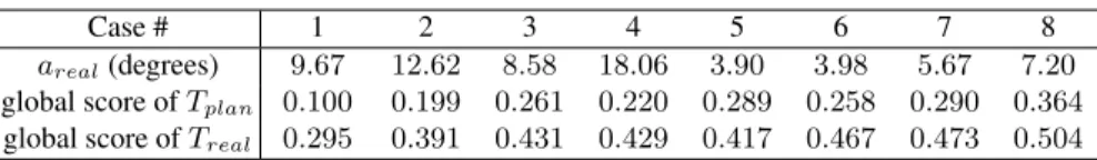
Table 2. Comparison between trajectory produced by our planning and reference trajectory
Case # 1 2 3 4 5 6 7 8 areal(degrees) 9.67 12.62 8.58 18.06 3.90 3.98 5.67 7.20
global score of Tplan 0.100 0.199 0.261 0.220 0.289 0.258 0.290 0.364
global score of Treal 0.295 0.391 0.431 0.429 0.417 0.467 0.473 0.504
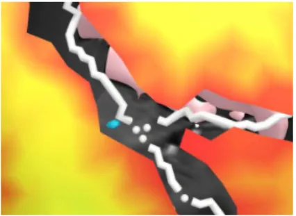
Fig.3 shows a detail of the color map of the risk constraint. The map has a bor-der where a trajectory towards the target (in blue) would meet any obstacle: here an approximation of a sulcal vessel represented by the white shape.
(a) Depth (b) Risk
(c) Orientation (d) Aggregative: kdepth = 2, krisk =
4, korient= 4
Fig. 2. Color maps of the soft constraints: best zones are in green and worst are in red (case #1).
In snapshot (d) the red line is the computed trajectory Tplan, and the green line is the reference
trajectory Treal
The experiments were performed on a 15” laptop, with a Dual Core CPU at 2.26 GHz and 4Go RAM, equipped with a NVIDIA GeForce Go 9300M GS GPU which is used to speed up occlusion queries. The constraint solving process and the generation of the colored maps and the optimal trajectory took less than 2 mn for each patient.
4
Discussion
We proposed a method able to provide valuable information for the neurosurgeon in the form of colored maps, that allow to see very quickly the individual scores of the possible insertion areas for each of the defined rules, facilitating the decision making. This method also computes an optimal path according to those rules, i.e. the path that has the best global score, result of the aggregative cost function, according to the cho-sen weightings. The computed angle arealdemonstrated that the trajectories performed
by the expert neurosurgeon were not so far from our proposed path (average of8.71 degrees), but not exactly the same. However in this kind of retrospective study it is dif-ficult to compare the results with the terrain truth, as the trajectories that were actually
Fig. 3. Detail of the risk map. The target is in
blue, the sulcal vessels in white, and the pink shape in the back is a part of the ventricles. The background is the grayscale MRI
Fig. 4. Color map of the aggregative soft
constraint, for different values of the weight-ing factors (case #1): kdepth = 1, krisk =
8, korient= 1. Tplanis at another location
used might not be the optimal ones. That is why we used constraints and weighting factors defined by the neurosurgeon, and computed the scores from them.
We can analyze the results in different ways. The weighting factors in the aggrega-tive cost function might have not been chosen at best, and might need to be refined to obtain a better fitting with their trajectory. Indeed, in many cases (5 over 8) the scores of constraint #6 (risk) are better for Tplan, and the scores of constraint #7 (orientation)
are better for Treal, suggesting that the optimization of the orientation of the electrode
relatively to the axis of the target may be of greater importance for the neurosurgeons than they thought when setting the weighting factors. However we can also say on the contrary that, as the rules and the weighting factors we used were defined by the neu-rosurgeons, the trajectories we plan better fit their theoretical criteria (the global scores of Tplanare better than the scores of Treal), and maybe the planning tool they used in
clinical routine did not provide them sufficient information and visibility for a correct selection.
An example of another possible computation with different weighting factors is shown on Fig.4 (kdepth = 1, krisk = 8, korient = 1). On this figure, the green line
representing Tplan is located in another place. On this example, we can notice that
there is one main green zone (where the optimal trajectory is located). The greatest part of the areas is orange/red, because we gave a higher weight to the risk constraint that colors in orange/red the borders of the possible insertion zone. This example, where the result differs completely from the one we used in our validation, illustrates how the result is highly dependent on an accurate choice of the weighting factors. That is why we plan in our future works to refine them.
We might also discover in the future that a constraint is implicitly used by the neu-rosurgeon but has not been expressed so far. In that case, one great advantage of our approach is the modularity. The new constraint only has to be translated into a cost function, formalized, and simply added into the constraints XML file, and it will be automatically taken into account in the next planning.
5
Conclusion
We described an approach using a geometric constraint solver fed with two types of input data: the formalization of the rules governing DBS planning and patient-specific images, to automatically compute an optimal placement for an electrode in the frame-work of assistance to DBS planning. The results we obtained show that the solutions proposed by our solver differed little from the solutions that were actually performed in clinical routine, but they had better scores regarding the rules defined by the surgeon themselves.
In the future we plan to feed the solver with other types of information, such as clinical scores, or predictions of the deformation of the electrode. Further clinical eval-uation with more surgical cases will also be performed, including other types of targets: globus pallidus internus (GPi) and ventral intermediate nucleus of the thalamus (VIM). Further works would also include the addition of new constraints that could be discov-ered and enunciated, especially when new targets will be considdiscov-ered. The modularity of our xml rule-based system will make that addition quite fast and convenient, as far as the new rules are clearly identified.
Acknowledgments
We would like to thank Florent Lalys from INRIA Rennes - Bretagne Atlantique, and Markus Engel from DKFZ Heidelberg (MITK) for their useful advices and help.
References
1. D’Haese, P.F., Cetinkaya, E., Konrad, P.E., Kao, C., Dawant, B.M.: Computer-aided place-ment of deep brain stimulators: from planningto intraoperative guidance. IEEE Trans. Med. Imaging 24(11) (2005) 1469–1478
2. Altrogge, I., Kr¨oger, T., Preusser, T., B¨uskens, C., Pereira, P., Schmidt, D., Weihusen, A., Peitgen, H.: Towards optimization of probe placement for radio-frequency ablation. In: MIC-CAI’2006. Volume 4190 of LNCS. (2006) 486–493
3. Lung, D., Stahovich, T., Rabin, Y.: Computerized planning for multiprobe cryosurgery using a force-field analogy. Comput. Meth. Biomech. Biomed. Eng. 7(2) (2004) 101–110
4. Adhami, L., Coste-Mani`ere, E.: Optimal planning for minimally invasive surgical robots. IEEE Transactions on Robotics and Automation 19(5) (2003) 854–863
5. Brunenberg, E., Vilanova, A., Visser-Vandewalle, V., Temel, Y., Ackermans, L., Platel, B., ter Haar Romeny, B.: Automatic trajectory planning for deep brain stimulation: A feasibility study. In: MICCAI’2007. Volume 4791 of LNCS. (2007) 584–592
6. Baegert, C., Villard, C., Schreck, P., Soler, L.: Multi-criteria trajectory planning for hepatic radiofrequency ablation. In: MICCAI’2007. Volume 4791 of LNCS. (2007) 584–592 7. Baegert, C., Villard, C., Schreck, P., Soler, L.: Trajectory optimization for the planning of
percutaneous radiofrequeny ablation on hepatic tumors. Computer Aided Surgery (2007) 8. Lalys, F., Haegelen, C., Abadie, A., Jannin, P.: Post-operative assessment in deep brain
stim-ulation based on multimodal images: registration workflow and validation. In: Medical Imag-ing: Vis., Image-Guided Procedures, and Modeling. Volume 7261(1)., SPIE (2009) 72612M