Learning Multicriteria Fuzzy Classification Method PROAFTN from Data

Publisher’s version / Version de l'éditeur:

Questions? Contact the NRC Publications Archive team at

PublicationsArchive-ArchivesPublications@nrc-cnrc.gc.ca. If you wish to email the authors directly, please see the first page of the publication for their contact information.

https://publications-cnrc.canada.ca/fra/droits

L’accès à ce site Web et l’utilisation de son contenu sont assujettis aux conditions présentées dans le site LISEZ CES CONDITIONS ATTENTIVEMENT AVANT D’UTILISER CE SITE WEB.

Computers and Operations Research Journal, 34, 7, pp. 1885-1898, 2005

READ THESE TERMS AND CONDITIONS CAREFULLY BEFORE USING THIS WEBSITE.

https://nrc-publications.canada.ca/eng/copyright

NRC Publications Archive Record / Notice des Archives des publications du CNRC : https://nrc-publications.canada.ca/eng/view/object/?id=ce2dc2ef-277f-40ee-a2d5-13d4aa4211bc https://publications-cnrc.canada.ca/fra/voir/objet/?id=ce2dc2ef-277f-40ee-a2d5-13d4aa4211bc

NRC Publications Archive

Archives des publications du CNRC

This publication could be one of several versions: author’s original, accepted manuscript or the publisher’s version. / La version de cette publication peut être l’une des suivantes : la version prépublication de l’auteur, la version acceptée du manuscrit ou la version de l’éditeur.

Access and use of this website and the material on it are subject to the Terms and Conditions set forth at

Learning Multicriteria Fuzzy Classification Method PROAFTN from Data

National Research Council Canada Institute for Information Technology Conseil national de recherches Canada Institut de technologie de l'information

Learning Multicriteria Fuzzy Classification

Method PROAFTN from Data *

Belacel, N., Raval. B. H., and Punnen, A. 2005

* published in Computers and Operations Research Journal. 2005. NRC 48254.

Copyright 2005 by

National Research Council of Canada

Permission is granted to quote short excerpts and to reproduce figures and tables from this report, provided that the source of such material is fully acknowledged.

Learning Multicriteria Fuzzy Classification

Method PROAFTN From Data

Nabil Belacel

∗, Hiral Bhasker Raval

and Abraham P Punnen

a

National Research Council Canada, Institute for Information

Technology-e-Business, 127 Carleton Street, Saint John, New Brunswick E2L 2Z6, Canada and Department of Mathematical Sciences, University of New Brunswick,

Saint John, New Brunswick, Canada

b

Department of Mathematical Sciences, University of New Brunswick, Saint John, New Brunswick, Canada

Abstract

In this paper, we present a new methodology for learning parameters of multiple criteria classification method PROAFTN from data. There are numerous represen-tations and techniques available for data mining, for example decision trees, rule bases, artificial neural networks, density estimation, regression and clustering. The PROAFTN method constitutes another approach for data mining. It belongs to the class of supervised learning algorithms and assigns membership degree of the alternatives to the classes. The PROAFTN method requires the elicitation of its pa-rameters for the purpose of classification. Therefore, we need an automatic method that helps us to establish these parameters from the given data with minimum clas-sification errors. Here we propose Variable Neighborhood Search metaheuristic for getting these parameters. The performances of the newly proposed method were evaluated using 10-cross validation technique. The results are compared with those obtained by other classification methods previously reported on the same data. It appears that the solutions of substantially better quality are obtained with proposed method than with these former ones.

Key words: Data mining, Multiple criteria classification, PROAFTN procedure, Variable neighborhood search

∗ Corresponding author. Address: National Research Council Canada, Institute for Information Technology-e-Business, 127 Carleton Street, Saint John, New Brunswick E2L 2Z6, Canada

Email addresses: nabil.belacel@nrc.gc.ca (Nabil Belacel), m89dz@unb.ca (Hiral Bhasker Raval), punnen@unbsj.ca (Abraham P Punnen).

1 Introduction

In many real-world decision problems, alternatives or objects are assigned to predefined classes, where the alternatives within each class are as similar as possible. For instance, in medical diagnosis, patients are assigned to disease classes according to set of symptoms. The problem of assigning alternatives to predefined classes in multiple criteria decision analysis (MCDA) is known as “multiple criteria sorting problems” [1]. This consists of the formulation of the decision problem in terms of the assignment of each object to one or several classes. The assignment is achieved through the examination of the intrinsic value of the objects by referring to pre-established norms, which correspond to vectors of scores on particular criteria or attributes, called profiles. These profiles can separate the classes or play the role of central reference points in the classes. Therefore, following the structure of the classes two situations can be distinguished: ordinal and nominal sorting problems [2]. The case where the classes are ordered is known as “ordinal sorting problems” and is charac-terized by a sequence of boundary reference objects. Scoring of credits is an example that can be treated using this problematic [3]. The case where the classes are not ordered is known as “nominal sorting problems” also called “multiple criteria classification problems” and is characterized by one or mul-tiple prototypes [4]. The prototype is described by a set of attributes and is considered as a good representative of its class.

Several outranking approaches to solving nominal and ordinal sorting prob-lems have been proposed in the literature. Among methods suggested for ordi-nal sorting problems are Trichotomic Segmentation [5] N-Tomic [6] and ELEC-TRE TRI [7]. Among methods proposed for solving multiple criteria classifica-tion problems are PROAFTN procedure [8] and more recently PROCFTN and k-Closest Resemblance procedures [9-10]. Other approaches based on the use of utility function [11] have also been proposed for ordinal sorting problems. Many of the above-mentioned approaches have been applied to the resolution of many real world practical problems including medical diagnosis [12-13], financial and economic management [3].

Outranking approaches exploit a preference model that is characterized by a number of parameters following more or less directly from preferential infor-mation supplied by the decision maker or expert. An outranking relation and parameters designate the preference model. The parameters consist of weights and various thresholds of attributes. The values assigned to these parame-ters will determine how the evaluation of alternatives according to different attributes should be combined. However, in many situations experts have dif-ficulty in defining precise values for preferential parameters due to various rea-sons. For example, data considered in the decision problem might be imprecise or uncertain; experts may have only a vague understanding of parameters and

their point of view can evolve during the elicitation process. This is why the idea of inferring preference models from examples has been very attractive. Therefore, several techniques using utility function and outranking relations have been proposed to infer preferential parameters [3, 11]. In general, these techniques proceed indirectly through a questioning procedure and translate expert answers into values that will be assigned to the preferential parameters. Other areas such as machine learning also use pre-assigned examples known as training set to infer the parameters of classification methods. Induction of rules or decision trees from examples [14-15] and learning approach from ex-amples for neural nets [16] are well-known representative methods of machine learning.

This paper will focus on a new multiple criteria classification method PROAFTN that has been recently developed [4, 8]. When using this method, we need to determine the values of several parameters (boundaries of intervals that define the prototype profiles, weights and thresholds. . . ). To determine these inter-vals we have used the general scheme of the discretization technique described by Ching et al. [17] that establishes a set of pre-classified cases called a training set. For parameters such as weights and discrimination thresholds, we apply a heuristic approach based on available knowledge and with the involvement of decision-makers. Even if these approaches offer good quality solutions, they still need considerable computational time and resources. In this study, we propose new approaches that infer parameters of the multiple criteria clas-sification procedure PROAFTN using training sets for solving clasclas-sification problems with very large data sets. This approach is based on Variable Neigh-borhood Search (VNS) Meta-heuristic proposed recently by Mladenovic and Hansen [18].

The rest of the paper is synthesized as follows: In the next section the PROAFTN method is introduced. Section 3 proposes a mathematical programming model of optimization PROAFTN parameters. In Section 4, the Chebyshev’s theo-rem with variable neighborhood search metaheuristic for determining the pa-rameters of PROAFTN method are presented. In section 5, Computational results on published medical test problems are presented. Conclusions and further works are discussed in Section 6.

2 PROAFTN _Method

In this section we briefly describe PROAFTN procedure (for detailed descrip-tion see references [4, 8]). PROAFTN method belongs to the class of super-vised learning and it is used for solving multiple criteria classification prob-lems. PROAFTN method has been applied to the resolution of many real world practical problems including medical diagnosis [12-13], asthma

treat-ments [19], docutreat-ments classification [20] and crew scheduling problem [21]. Let each object, which we need to classify, is described by a set of m at-tributes {g1, g2. . . gm} and let {C

1

. . . Ck_{} be the set of k classes. Given an} object a, described by the score of m attributes, the different steps of the procedure are as follows:

Initialization

For each class Ch_{, h =1, 2...k, we determine a set of Lh prototypes B}h ₌ {bh

1, bh2,. . . ,bh_Lh} using the available knowledge (from the decision maker or

from the pre-assigned data set known as training set). The prototypes are considered to be good representatives of their class and are described by the score upon each of the m attributes. More precisely, to each prototype bh

i and each attribute gj, j= 1, 2,. . . , m; an interval [S1

j(bhi), S 2 j(bhi)] is defined with S2 j(bhi) ≥ S 1 j(bhi), j = 1,2..,m; h=1,2,. . . ,k and i= 1,2,. . . , Lh.

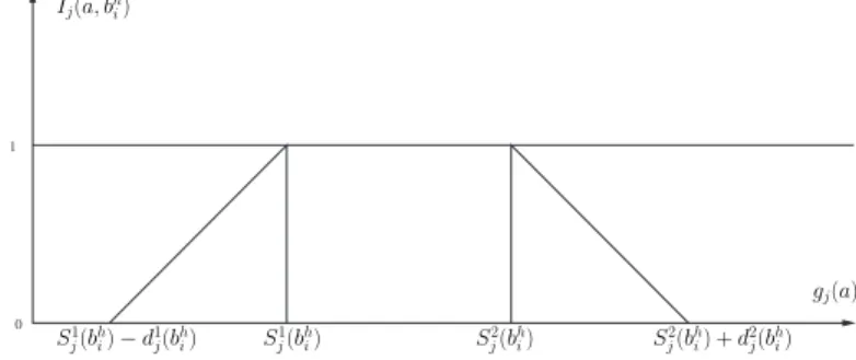
When evaluating a certain quantity or a measure with a regular (crisp) inter-val, there are two extreme cases, which we should try to avoid. It is possible to make a pessimistic evaluation, but then the interval will appear wider. It is also possible to make an optimistic evaluation, but then there will be a risk of the output measure to get out of limits of the resulting narrow interval, so that the reliability of obtained results will be doubtful. Fuzzy intervals do not have these problems. They permit to have simultaneously both pessimistic and optimistic representations of the studied measure [22]. This is why we introduce the thresholds d1

j(bhi) and d 2

j(bhi) to define in the same time the pes-simistic interval [S1

j(bhi), S 2

j(bhi)] and the optimistic interval [S 1 j(bhi) − d 1 j(bhi), S2 j(bhi) + d 2

j(bhi)]. The carrier of a fuzzy interval (from S 1

minus d1 to S2

plus d2

) will be chosen so that it guarantees not to override the considered quantity over necessary limits, and the kernel (S1

to S2

) will contain the most true-like values (see Fig: 1).

1 0 Ij(a, bhi) gj(a) S2 j(bhi) + d2j(bhi) S2 j(bhi) S1 j(bhi) S1 j(bhi) − d1j(bhi)

Fig. 1. Graphical representation of the partial indifference (partial concordance) index between the object a and prototype bh

i. This graph assumes continuity and

linear interpolation

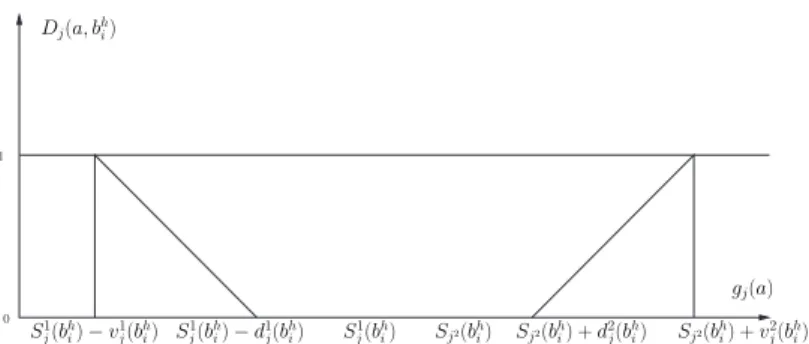
dis-1 0 Dj(a, bhi) gj(a) Sj2(bh i) + vj2(bhi) Sj2(bh i) + d2j(bhi) Sj2(bh i) S1 j(bhi) S1 j(bhi) − d1j(bhi) S1 j(bhi) − v1j(bhi)

Fig. 2. Graphical representation of the partial discordance index to the indifference relation between the object aand prototype bh

i. This graph assumes continuity and

linear interpolation.

cretization technique described by Ching et al. [17] that establishes a set of pre-classified cases called a training set. In addition, we assign values to the parameters (weights, veto thresholds), which are used in calculating the mem-bership degree of the object to be assigned to the class.

Computing the fuzzy indifference relation

For classification of the object a, PROAFTN method calculates the indiffer-ence relation I(a, bh

i), h =1, 2. . . , k and i = 1,2. . . Lh on the basis of concor-dance and non-discorconcor-dance principles [4, 8]. The indifference relation basically gives us the degree of validation of the statement “a and bh

i are indifferent or roughly equivalent”. Using the principle of concordance and non-discordance, the indifference index is calculated by

I(a, bhi) = ( m X j=1 wjhIj(a, b h i)) m Y j=1 (1 − Dj(a, bhi)w h j) (1) where wh

j is the positive coefficient stating the relative importance attached by a decision maker to an attribute gj of the class Ch_.

Ij(a, bh

i), j=1,2,..,.m, is the degree with which attribute gj is in favor of the indifference relationship between a and bh

i. For calculating this, two positive discrimination threshold d1

j(bhi) and d 2

j(bhi) are used to take into account the imprecision in the data.

Dj(a, bh

i) j=1, 2. . . m is the degree with which attribute gj is against the indifference relation between a and bh

i. For this, two veto thresholds v 1 j(bhi) and v2

j(bhi), j=1, 2,...,m, are used to define the values from which the object a is considered as very different from the prototype bh

i according to attribute gj.

The above equation (1) shows that this index increases with the quantities Ij(a, bh

anal-ysis of all these indices, see [4, 8]. Throughout this paper we set the veto thresholds in infinity so that the formula 1 becomes:

I(a, bh i) = ( m X j=1 wh jIj(a, b h i)) (2)

Evaluate the degree of membership µ(a, Ch₎

The degree of the membership of an object a to class Ch_{, h=1, 2,...,k is} measured by the indifference degrees between a and its nearest neighbor in Bh _{according to fuzzy indifference relation I:}

µ(a, Ch_{) = max {I(a,b}h

1), I(a, bh2), . . . , I (a, bh_Lh)}, h=1, 2,. . . ,k

Assignment of an object

After calculating the degree of membership µ(a, Ch_{), h=1, 2. . . k, the} assign-ment decision is made by:

a ∈ Ch _{⇔ µ(a, C}h_{) = max{µ(a, C}l_{)/l ∈{1,2. . . k}}}

3 Problem Description

For a given multiple criteria classification problem, to apply PROAFTN we need to infer the interval [S1

j(bhj) − d 1 j(bhj), S 2 j(bhj) − d 2

j(bhj)] for each attribute in the given class. For our problem we assume weights for all attribute to be equal. Basically there are two methods to elicit these parameters: Direct Technique and Indirect Technique. In the first technique to elicit the required information of these parameters we need to have interactive interrogation with the decision maker for whom we are solving the problem. The interaction with the decision-maker ensures that his/her preferences are properly presented in the model. However this technique is often time-consuming and it is subject to the decision-maker willingness to participate in such an interactive process or not. Also for some problems we may not have the decision maker but only the dataset regarding the problem is available. In such case second technique helps out. That is we need some automatic techniques to get these parameters from the available data of the problem. Sometimes, this is referred to as pref-erence disaggregation approach [3-11]. In this, from the set of examples known as training set, we extract the necessary preferential information required to construct a classifier and use these for assigning the new cases. It is similar to use of training sample for model development as in machine learning. All

these approaches share a common ground, i.e. the use of existing knowledge represented in a training sample for model development [14-17].

For our problem also, instead of using direct procedure, a preference disag-gregation approach is used for adjusting parameters {S1

, S2 }, {q1 , q2 }, where S1 = S1 j(bhi); S 2 = S2 j(bhi); q 1 = S1 j(bhi) − d 1 j(bhi) and q 2 = S2 j(bhi) + d 2 j(bhi)for any attribute gj and for any prototype bh

i. The parameters {S1

, S2 , q1

, q2

} can be obtained by solving the following math-ematical programming problem

P: Minimize n X i=1 k X h=1 (µih(S1 jh, S 2 jh, q 1 jh, q 2 jh) − αih) 2 (3) Subject to Sjh1 − q 1 jh ≤ S 2 jh+ q 2 jh; j = 1, 2, ..., m; h = 1, 2, . . . , k; S1 jh ≥ 0, S 2 jh ≥ 0; q 1 jh ≥ 0, q 2 jh ≥ 0; j = 1, ..., m; h = 1, . . ., k

The above objective function (3) consists in minimizing the classification errors (i.e. minimize the difference between the membership value µih(S1

, S2 , q1

, q2 ) obtained by fuzzy classification method PROAFTN with the value of the as-signment index αihgiven a priori in the training set. For example, if the index αih= 1, then the value of the membership degree µih should be close to 1 and all other value of the membership degree µil, for l 6= h, should be close to zero. The set of parameters {S1

, S2 , q1

, q2

} represent the decision variables (i.e., the optimal value of set {S1

, S2 , q1

, q2

} is obtained as a solution of the non-linear programming problem (P)). Since the objective function (3) is nei-ther convex nor concave and usually has many local optima, so, finding global optimum of (P) appears to be very difficult. Hence, it is very hard to solve the mathematical programming (P) using the classical methods such as gra-dient algorithms, generalized reduced method and interior-point algorithms. Therefore, we will adapt the Chebyshev’s theorem and meta-heuristic variable neighborhood search (VNS) to solve the non-linear programming (P) in or-der to infer parameters of multiple classification method PROAFTN. In the next section we will describe the developed algorithms to infer the PROAFTN parameters.

4 Developed Algorithms for learning PROAFTN method

The developed algorithm to solve the mathematical programming (P) is es-sentially based on VNS metaheuristics proposed by Mladenovic and Hansen [18]. It should be noted that the initial solution for this problem is obtained using the Chebyshev’s theorem, which is described in the next section.

4.1 Application of Chebyshev’s theorem for finding prototypes in PROAFTN method

In this section we will present an approach based on Chebyshev’s theorem for adjusting parameters for PROAFTN method. Before developing in detail how the parameters of PROAFTN method are determined, we point out a very important theorem that will be adapted to our context as follows [23]:

Chebyshev’s theorem. For any data distribution, at least 100(1-1/t2 ) % of the objects in any data set will be within t standard deviations of the mean, where t is greater than 1.

The main advantage of Chebyshev’s theorem is that it can be applied to any shape distribution of data [23].

The prototypes are considered to be good representatives of their class and are described by the score upon each of the m attributes. More precisely, to each prototype bh

i and each attribute gj, j= 1, 2,. . . , m; an interval [S 1 j(bhi), S 2 j(bhi)] is defined with S2 j(bhi) ≥ S 1 j(bhi), j= 1,2..m; h=1,2. . . .k and i= 1,2,. . . , Lh. To determine these intervals we have used Chebyshev’s theorem described above. Suppose we have a training set consisting of instances (objects) which are described by some attributes. To determine the intervals [S1

, S2

] considered as pessimistic intervals and [q1

, q2

] as optimistic intervals, we have applied the following algorithm:

ALGORITHM 1. (Chebyshev’s theorem for PROAFTN method) For each class in training set

1) For each attribute in it, first calculate the mean (x) and standard deviation (σ).

2) For t= 2, 3, 4, 5

For each attribute, calculate the percentage of values which are between x±tσ If percentage ≥ (1 − 1/t2

first interval i.e. S1

= x-tσ, S2

= x+t σ, q1

= x-(t+1) σ, q2

= x+ (t+1) σ otherwise go to next value of t.

The algorithm1 allows us to determine the intervals [S1 , S2

] called pessimistic intervals and also the discrimination thresholds [q1

, q2

] called optimistic inter-vals. These intervals define the prototypes of the classes. Submit these intervals to the PROAFTN method for calculating the indifference relation between prototypes and the different cases to be assigned to the classes as described in section 2. This solution is approximate and there is no guarantee that the solution is good. We alleviate this difficulty by using Variable Neighborhood Search (VNS) heuristic to improve further on the solution found, which is presented in the next section.

4.2 Variable neighborhood search for inferring P ROAF T N parameters

Variable Neighbourhood Search (VNS) is a recently proposed metaheuristic for solving combinatorial and global optimisation problems [18]. The basic idea is to proceed to a systematic change of neighbourhood within a local search algorithm. This algorithm remains in the same locally optimal solution exploring increasingly far neighbourhoods of it by random generation of a point and descent, until another solution better than the incumbent is found. When so, it ”jumps” there, i.e., contrary to simulated annealing or Tabu search [24], it is not a trajectory following method.

The basic VNS [18] is very useful for approximate solution of many combina-torial and global optimization problems but still it remains difficult or long to solve very large instance. Usually the most time-consuming ingredient of basic VNS is the local search routine which it uses. A drastic change is pro-posed in Reduced VNS (RVNS) [25-26]. Thus in RVNS, solutions are drawn at random in increasingly far neighborhoods of the incumbent and replace it if and only if they give a better objective function value. In many cases, this simple scheme of RVNS provides good results, in very moderate time [25]. The general algorithm for Reduced VNS is as follows:

ALGORITHM 2 (RVNS algorithm):

Initialization: Select the set of neighborhood structures Nk, for k=1, 2,. . . , kmax, that will be used in the search; find an initial solution x; choose a stopping condition;

Repeat the following sequence until the stopping condition is met; Set k =1

Repeat the following steps until k = kmax

Shaking: Generate a point x′ _{at random from the k}th _{neighborhood of x (x}′ _∈ Nk(x))

Move or not: If this point is better than the incumbent; move there (x = x′₎ and continue the search with N1(k = 1); otherwise set k = k + 1

RVNS is very useful for very large instances for which local search is costly. Here the stopping condition may be maximum CPU time, maximum number of iteration or maximum number of iterations between two improvements. We have applied the above RVNS algorithm to infer the parameters of PROAFTN method with minimum classification errors i.e. to infer near-optimal parame-ters and correctly classify the test data.

The different steps of RVNS using Chebyshev’s theorem to find initial solution are presented as follows:

ALGORITHM 3 (RVNS for PROAFTN method):

Initialization: From training set and by using Algorithm1 (N1) assign the initial values to parameter set {S1

, S2 , q1

, q2

} for each attribute. Calculate the ob-jective function value f (correctly classified percentage) by submitting these values to PROAFTN method. Choose the stopping condition as maximum CPU time and kmax (number of parameters, here it is 4).

Repeat: Following sequences until stopping condition is met: Set k = 1 (number of parameter to be generated)

Repeat the following until k > kmax :

Shaking: For each attribute, generate a random number j between 1 and kmax and then again generate jth_{parameter from k}th _{neighborhood. For example, if} k = 1, then generate randomly only one parameter for each attribute. If k = 2, then generate in same time two parameters (which parameter to generate depends on the number j generated between 1 and kmax ). Submit the new parameters generated randomly to PROAFTN method to calculate the new objective function value f′_.

Move or not: If f ’ > f, then take the current parameter and continue the search with N1 (k =1); otherwise set k = k+1.

5 Application of the Developed Algorithm

We have applied the above heuristics to four health related dataset: Wisconsin Breast Cancer, Pima Indian Diabetics, Cleveland Heart Disease and Hepatitis Dataset. All these datasets are available on public domain of University of California at Irvine (UCI) repository database

(http: //www.ics.uci.edu/∼mlearn/MLRepository.html). All algorithms are coded in C++ and run on Dell-Intel r° XeonTM

CPU 3.06 GHZ, 1.00 GB of RAM. Each dataset was randomly distributed into a set containing 2/3rd _of the instances as training and another set containing the remaining 1/3rd _for testing. We have applied PROAFTN with Chebyshev’s and also PROAFTN with RVNS by using solutions obtained by Chebyshev’s as initial solution on these four data sets.

The algorithms were tested on ten different random splits and the results presents the average of correct classification accuracy. Description and results of each dataset is given below:

Wisconsin Breast Cancer: This dataset involves classifying breast cancer cases from University of Wisconsin at Madison Hospital as either benign or malignant.

Number of Instances: 699 Number of Attributes: 10

Name of Attributes: Sample code number, clump thickness, uniformity of cell size, uniformity of cell shape, marginal adhesion, single epithelial cell size, bare nuclei, bland chromatin, normal nucleoli and mitosis.

Number of Classes: 2 (benign-458 and malignant-241) Results

This is the most common database used to test the performances of the clas-sifiers. Table 1 summarizes results of the comparison between our developed methods with 10 other classifiers including: Multi-Stream Dependency Detec-tion algorithm; 1- Nearest neighbour; two pairs of parallel hyperplanes (1 trial only); three pairs of parallel hyperplanes (1 trial only); neural network; linear discriminant; decision tree (ID3); Bayes (second order); quadratic discrimi-nant.

From the table 1 we can see that when PROAFTN is used with RVNS (97.9 % of correct classification), it outperforms other classifier like 1-nearest neighbor

Table 1

Comparative results on Wisconsin Breast Cancer data for five classifiers for the eleven classifiers: (1. PROAFTN with Chebyshev; 2. PROAFTN with RVNS; 3. Multi-Stream Dependency Detection algorithm (MSDD); 4. 1-Nearest Neighbor (1-NN); 5. Two pairs of parallel hyperplanes (2-PPH); 6. Three pairs of parallel hy-perplanes (3-PPH); 7. Neural network; 8. Linear Discriminant; 9. Decision tree ID3; 10. Bayes (second order); 11. Quadratic Discriminant.

Correctly Classified % Reference 1 PROAFTN with Chebyshev 96.1

2 PROAFTN with RVNS 97.9 3 MSDD algorithm 95.2 [27] 4 1- NN 93.7 [28] 5 2-PPH (1 trial only) 93.5 [29] 6 3-PPH (1 trial only) 95.9 [29] 7 Neural network 71.5 [30] 8 Linear Discriminant 71.6 [30]

9 Decision tree ID3 69.3 [31]

10 Bayes (second order) 65.6 [30] 11 Quadratic Discriminant 65.6 [30]

(93.7%), two and three pairs of parallel hyperplanes (93.5%, 93.9%), neural nets (71.5%), ID3 (69.3%), etc.

Pima Indian Diabetics: This dataset involves in identifying patients who show the signs of diabetics according to the World Health Organization (WHO) criteria. It was originally taken from National Institute of Diabetics and Di-gestive and Kidney Disease.

Number of Instances: 768 Number of Attributes: 8

Name of Attributes: Number of times pregnant, plasma glucose concentration, diastolic blood pressure (mm Hg), triceps skin fold thickness (mm), 2-Hour serum insulin (mu U/ml), body mass index, diabetes pedigree function and age.

Number of Classes: 2 (Not tested positive-500 and tested positive-268) Results

In Table 2 we can see that when we apply PROAFTN with Chebyshev’s it only gives 21.715% of correctly classified but by applying PROAFTN with RVNS using the PROAFTN starting with Chebyshev’s solution, the percentage of correct classification increase to 72.4185%. As stated by other researchers, this is the most difficult dataset for classification. From our developed algorithm we get better or near about similar results when compared to other classifiers.

Table 2

Comparative results on Pima Indian Diabetics for four classifiers (1. PROAFTN with Chebyshev; 2. PROAFTN with RVNS; 3. Multi-Stream Dependency Detection algorithm (MSDD);ADAP learning algorithm.

Correctly Classified % Reference 1 PROAFTN with Chebyshev 21.7

2 PROAFTN with RVNS 72.4

3 MSDD algorithm 71.3 [27]

4 ADAP learning algorithm 76 [32]

Cleveland Heart Disease: This dataset involves in separating patients who have heart disease and those who do not. It was originally obtained from Cleveland Clinic Foundation. This database contains 76 raw attributes but all published experiments refer to using a subset of 13 relevant of them.

Number of Instances: 303 Number of Attributes: 13

Name of Attributes: Age, Sex, chest pain type, resting blood pressure, choles-terol, fasting blood sugar, resting electrocardiography results, maximum heart rate received, exercise induced angina, ST depression induced by exercise rel-ative to rest, slope of the peak exercise ST segment, number of major vessels coloured by fluoroscopy, thal.

Number of Classes: 2 (absence- 164 and presence-139) Results

Table 3 shows comparative results between our developed algorithms with five other classifiers including Multi-Stream Dependency Detection algorithm; Backpropagation; 3-nearest neighbour; decision tree C4.5 (pruned); decision tree ID3. As we can see at the table 3 our algorithm (PROAFTN with RVNS) outperforms the other classifiers with the percentage of correctly classified was 88.3107. On the other hand the other classifiers get the following results: Backpropagation (80.6%), 3-nearest neighbor (79.2%), C4-pruned (74.8%), ID3 (71.2%)).

Table 3

Comparative results on Cleveland Heart Disease for the seven classifiers (1. PROAFTN with Chebyshev; 2. PROAFTN with RVNS; 3. Multi-Stream Depen-dency Detection algorithm (MSDD); 4. Backpropagation algorithm; 5. 3-nearest neighbor (3-NN); 6. Decision tree C4.5 (pruned); 7. Decision tree ID3.

Correctly Classified % Reference 1 PROAFTN with Chebyshev 73.161

2 PROAFTN with RVNS 88.3107 3 MSDD algorithm 79.21 [27] 4 Backpropagation 80.6 [33] 5 3-nearest neighbour 79.2 [34] 6 C4.5 (pruned) 74.8 [35] 7 ID3 71.2 [33]

Hepatitis Dataset: This dataset requires determination of whether patients with hepatitis will either live or die. It was donated by Jozef Stefan Institute, Yugoslavia.

Number of Instances: 155 Number of Attributes: 19

Name of Attributes: Age, Sex, steroid, antivirals, fatigue, malaise, anorexia, liver big, liver firm, spleen palpable, spiders, ascites, varices, bilirubin, alk phosphate, sgot, albumin, protime, histology

Number of Classes: 2 (Die-32 and Live-123) Results:

Table 4 summarizes results of the comparison between our developed methods with four other classifiers including Multi-Stream Dependency Detection algo-rithm; Assistant(pre-punning) ; C4 decision tree(pruned); C4 decision tree (un-pruned tree). As shown in the Table 4 when we apply PROAFTN with Cheby-shev’s, we get only 64.4 % of correctly classified. But on applying PROAFTN with RVNS, the percentage increases to 85.575 which also outperform the other classifiers like multi-stream dependency detection algorithm (80.77%), ASSISTANT (83%) and C4 decision tree (81.2%).

Note that the maximum time allowed for each run (tmax) is given for RVNS as 2 seconds for the all above applications. So, the possibility of some further small improvement with a much larger tmax cannot be ruled out.

Table 4

Comparative results on Hepatitis Dataset for the six classifiers (1. PROAFTN with Chebyshev; 2. PROAFTN with RVNS; 3. Multi-Stream Dependency Detection al-gorithm (MSDD); 4. Assistance ; 5. Decision tree C4 (pruned); 6. Decision tree ID3.

Correctly Classified % Reference 1 PROAFTN with Chebyshev 64.4

2 PROAFTN with RVNS 85.8

3 MSDD algorithm 80.8 [27]

4 ASSISTANT algorithm 83 [36]

5 C4 decision tree (pruned) 81.2 [37]

6 C4 decision tree 79.3 [38]

6 Conclusions and Future Work

In this paper, we have proposed a new approach for inferring parameters of fuzzy multiple criteria classification method PROAFTN. This approach is based on Chebyshev’s rules and used the metaheuristic RVNS. The improved classifier PROAFTN method was tested on different health related datasets which provided better results when compared with other classifiers reported previously by other researchers. To the best of our knowledge, no research has been proposed that would infer parameters of the preferential model in multiple criteria classification or nominal sorting problems. When RVNS is used with PROAFTN, it has several advantages for data modeling. Firstly, the method uses multiple criteria decision analysis and hence can be used to gain understanding about the problem domain. Secondly, as PROAFTN has both a direct and automatic technique to fit parameters, it is ideal method for combining prior knowledge and data. Thirdly, it provides possibility to have access to more detailed information concerning the classification decision. For assignment, the fuzzy membership degree gives us idea about its “weak” and “strong” membership to the corresponding classes.

Comparative testing on several problems demonstrates that the proposed method PROAFTN with RVNS outperforms the classical classification meth-ods previously reported on the same data and the used the same validation technique (10-fold cross validation technique). Further developments of the procedure include the following research directions: (i) apply other meta-heuristics such as Tabu search, genetics algorithms, simulated annealing to infer PROAFTN parameters from training set ; (ii) extend the developed methodology to take into account the veto phenomenon and the weights of the attributes considered in the complete version of the PROAFTN method; (iii) combine PROAFTN and VNS for multiple criteria classification problem

with decomposition for solving very large instances; (iv) build parallel ver-sions of these heuristics; (v) apply enhanced heuristics to further real world problems from pattern recognition, image analysis, astrophysics and bioinfor-matics.

Acknowledgements.

We are thankful to the referees for their comments which improved the presen-tation of the paper. This work was partially supported by NSERC discovery grants awarded to Nabil Belacel and Abraham P Punnen and partially funded by NRC, IIT e-health.

References

(1) B. Roy. Multi-criteria methodology for decision aiding, non-convex op-timization and its applications. Kluwer Academic Publishers, Dordrecht (1996).

(2) C. Zopounidis, M. Doumpos. Multicriteria classification and sorting meth-ods: A literature review. European Journal of Operational Research 138 2 (2002), pp. 229-246.

(3) C. Zopounidis, M. Doumpos, The use of the preference disaggregation analysis in the assessment of financial risks, Fuzzy Economic Review 3 1 (1998), 39-57.

(4) N. Belacel. M´ethodes de classification multicrit`ere: M´ethodologie et appli-cation `a l’aide au diagnostic m´edical, Ph.D. Disertation, Free University of Brussels, Belgium, 1999.

(5) B. Roy and J. Moscarola, Proc´edure automatique d’examen de dossiers fond´ee sur une segmentation trichotomique en pr´esence de crit`eres mul-tiples. RAIRO Recherche Op´erationnele 11 2 (1977), pp. 145–173. (6) M Massaglia, A. Ostanello. N-TOMIC: a decision support for

multicrite-ria segmentation problems. In: Korhonen P, editor. International Work-shop on Multicriteria Decision Support. Lecture Notes in Economics and Mathematics Systems 356. Berlin: Springer, 1991. p. 167–74.

(7) V. Mousseau, R. Slowinski and P. Zielniewicz, A user-oriented implemen-tation of the ELECTRE-TRI method integrating preference eliciimplemen-tation support. Computers and Operations Research 27 7-8 (2000), pp. 757– 777.

(8) N. Belacel, Multicriteria assignment method PROAFTN : Methodology and medical applications. European Journal of Operational Research 125 (2000), pp.175-183.

(9) N. Belacel, M.R. Boulassel. Multicriteria fuzzy classification procedure PROCFTN: methodology and medical application. Fuzzy Sets and Sys-tems 141 2 (2004), pp. 203–217.

(10) N. Belacel. The k-Closest Resemblance Approach for Multiple Criteria Classification problems. In L. T. Hoai, P. D. Tao (Eds.). Modeling,

Com-putation and Optimization Information and Management Sciences. Her-mes Sciences Publishing, 2004. p. 525-534.

(11) Y. Siskos et al. Measuring customer satisfaction using a survey based preference disaggregation model. Journal of Global Optimization 12 2 (2000), pp. 175-195.

(12) N. Belacel, M.R Boulassel. PROAFTN classification method: A useful tool to assist medical diagnosis. Artificial Intelligence in Medicine 21 1-3 (2001), pp. 199-205.

(13) N. Belacel, Ph. Vincke, J.M. Scheiff, M. R. Boulassel. Acute leukemia di-agnosis aid using multicriteria fuzzy assignment methodology. Computer Methods and Programs in Biomedicine 64 2 (2001), pp. 145-151.

(14) R.S. Michalski. A theory and methodology of inductive learning. Artificial Intelligence 20 (1983), pp.11-116.

(15) S.M. Weiss, C.A. Kulikowski Computer systems that learn. Morgan Kauf-mann, San Mateo, 1991.

(16) .P. Arhcer, S. Wang Application of the back propagation neural networks algorithm with monotonicity constraints for two group classification prob-lems. Decision Sciences 24 (1993), pp. 60-75.

(17) J.Y. Ching et al. Class-dependent discretization for inductive learning from continuous and mixed-mode data. IEEE Trans. Pattern Anal. Mach. Intell. 7 (1995), pp. 641–651.

(18) N. Mladenovic, P. Hansen, Variable neighborhood search: Principles and applications, European J. Oper. Res. 130 (2001), pp. 449-467.

(19) F. J. Sobrado, J. M. Pikatza, I. U. Larburu, J. J. Garcia, D. de Ipi˜na. Towards a Clinical Practice Guideline Implementation for Asthma Treat-ment. In R. Conejo, M. Urretavizcaya, J. P´erez-de-la-Cruz (Eds.) Cur-rent Topics in Artificial Intelligence: 10th Conference of the Spanish As-sociation for Artificial Intelligence, Lecture Notes in Computer Science Springer-Verlag Heidelberg, 2004, p. 587-596.

(20) A. Guitouni, B. Brisset, L. Belfares., K. Tiliki, N. Belacel, C. Poirier, P. Bilodeau, Automatic Documents Analyzer and Classification, Proc. of 7th International Command and Control Research Technology Symposium, Sept. 16-20, 2002.

(21) H. Ait-Hamou, S´election des pilotes pour une r´e-optimisation suite `a des perturbations, M.Sc Disertation, D´epartement de Math´ematiques et de G´enie Industriel, ´Ecole Polytechnique de Montr´eal, 2001.

(22) D. Dubois, H. Prade and R. Sabbadin, Decision-theoretic foundations of possibility theory. European J. Oper. Res. 128 (2001), pp. 459–478. (23) H.R. Gibson. Elementary statistics. Wm.C. Brown Publishers, 1994. (24) I.H Osman., G. Laporte. Metaheuristic: A bibliography, Annals of

Oper-ation Research 63 (1996), pp. 513-628.

(25) P. Hansen, N. Mladenovic, D. Perez-Britos. Variable Neighborhood De-composition Search. Journal of Heuristics 7 4 (2001), pp. 335-350. (26) P. Hansen, N. Mladenovic. Developments in Variable Neighbourhood

Meta-heuristics, Kluwer Academic Publishers, Dordrecht, 2002, p. 415-439. (27) T. Oates, MSDD as a Tool for Classification, Research Report,

Exper-imental Knowledge Systems Laboratory, Department of Computer Sci-ence, University of Massachusetts, Amherst, 94-29, 1994.

(28) J. Zhang. Selecting typical instances in instance-based learning. In: Pro-ceedings of ninth international machine learning conference, Aberdeen, Scotland: Morgan Kaufmann, 1992, p. 470-479.

(29) W.H. Wolberg, O.L. Mangasarian. Multisurface method of pattern sep-aration for medical diagnosis applied to breast cytology. In: Proceedings of National Academy of Sciences 87, 1990, p. 9193-9196.

(30) S.M. Weiss, I. Kapouleas. An empirical comparison of pattern recogni-tion, neural nets and machine learning classification methods. In: Pro-ceedings of the Eleventh International Joint Conference on Artificial In-telligence, San Mateo, CA: Morgan Kaufmann, 1989, P. 688-693.

(31) M. Tan, L. Eshelman. Using weighted networks to represent classification knowledge in noisy domains. In: J. Laird (Eds.), Proceedings of the Fifth International Conference on Machine Learning, San Mateo, CA: Morgan Kaufmann, 1988, p.121-134.

(32) J.W. Smith, J.E. Everhart, W.C. Dickson, W.C. Knowler, R.S. Johannes. Using the ADAP learning algorithm to forecast the onset of diabetics mellitus. In: Proceedings on 12th _{Symposium on Computer Applications} in medical care, R.A. Greenes (Ed.), IEEE Computer Society Press, 1988, p. 261-265.

(33) J. Shavlik, R.J. Mooney, G. Towell. Symbolic and neural learning algo-rithms: An experimental comparison. Machine Learning 6 (1991), pp. 111-143.

(34) D.W Aha, D. Kibler. Noise-tolerant instance-based learning algorithms. In: Proceedings of the Eleventh International Joint Conference on Arti-ficial Intelligence, San Mateo, CA: Morgan Kaufmann, 1989, p.794-799. (35) D. Kibler, D.W. Aha. Comparing instance-averaging with instance-filtering

learning algorithms. In: D. Sleeman (Eds.), EWSL88: Proceedings of the 3rd _{European Working Session on Learning, (1988), p. 63-69.}

(36) E. Cestnik, I. Konenenko, I. Bratko. Assistant-86: A knowledge elicitation tool for sophisticated users. In: I. Brato & N.Lavrac (Eds.), Progress in Machine Learning, Wilmslow, England, Sigma Press, (1987), p. 31-45. (37) Holte, C. Robert. Very simple classification rules perform well on most

commonly used data sets. Machine Learning 11 (1993), pp. 63-91. (38) P. Clark, R. Boswell. Rule induction with CN2: Some recent

improve-ments. In: Y. Kodratoff (Eds.), Machine Learning-EWSL-91, Springer-Verlag, (1991), p. 151-163.