arXiv:1107.0882v2 [hep-ex] 13 Jul 2011
EUROPEAN ORGANIZATION FOR NUCLEAR RESEARCH (CERN)
LHCb-PAPER-2011-005 CERN-PH-EP-2011-082 October 30, 2018
Measurement of V
0
production ratios
in pp collisions at
√s = 0.9 and 7 TeV
The LHCb Collaboration1
Abstract
The Λ/Λ and Λ/K0
S production ratios are measured by the LHCb detector from
0.3 nb−1 of pp collisions delivered by the LHC at √s = 0.9 TeV and 1.8 nb−1 at
√s = 7 TeV. Both ratios are presented as a function of transverse momentum, p
T,
and rapidity, y, in the ranges 0.15 < pT< 2.50 GeV/c and 2.0 < y < 4.5. Results at the
two energies are in good agreement as a function of rapidity loss, ∆y = ybeam− y, and
are consistent with previous measurements. The ratio Λ/Λ, measuring the transport of baryon number from the collision into the detector, is smaller in data than predicted
in simulation, particularly at high rapidity. The ratio Λ/K0
S, measuring the
baryon-to-meson suppression in strange quark hadronisation, is significantly larger than expected.
1
The LHCb Collaboration
R. Aaij23, B. Adeva36, M. Adinolfi42, C. Adrover6, A. Affolder48, Z. Ajaltouni5, J. Albrecht37,
F. Alessio6,37, M. Alexander47, G. Alkhazov29, P. Alvarez Cartelle36, A.A. Alves Jr22, S. Amato2,
Y. Amhis38, J. Anderson39, R.B. Appleby50, O. Aquines Gutierrez10, L. Arrabito53,
A. Artamonov34, M. Artuso52,37, E. Aslanides6, G. Auriemma22,m, S. Bachmann11, J.J. Back44,
D.S. Bailey50, V. Balagura30,37, W. Baldini16, R.J. Barlow50, C. Barschel37, S. Barsuk7,
W. Barter43, A. Bates47, C. Bauer10, Th. Bauer23, A. Bay38, I. Bediaga1, K. Belous34,
I. Belyaev30,37, E. Ben-Haim8, M. Benayoun8, G. Bencivenni18, S. Benson46, R. Bernet39,
M.-O. Bettler17,37, M. van Beuzekom23, A. Bien11, S. Bifani12, A. Bizzeti17,h, P.M. Bjørnstad50,
T. Blake49, F. Blanc38, C. Blanks49, J. Blouw11, S. Blusk52, A. Bobrov33, V. Bocci22,
A. Bondar33, N. Bondar29, W. Bonivento15, S. Borghi47, A. Borgia52, T.J.V. Bowcock48,
C. Bozzi16, T. Brambach9, J. van den Brand24, J. Bressieux38, D. Brett50, S. Brisbane51,
M. Britsch10, T. Britton52, N.H. Brook42, A. B¨uchler-Germann39, I. Burducea28, A. Bursche39,
J. Buytaert37, S. Cadeddu15, J.M. Caicedo Carvajal37, O. Callot7, M. Calvi20,j,
M. Calvo Gomez35,n, A. Camboni35, P. Campana18,37, A. Carbone14, G. Carboni21,k,
R. Cardinale19,i, A. Cardini15, L. Carson36, K. Carvalho Akiba23, G. Casse48, M. Cattaneo37,
M. Charles51, Ph. Charpentier37, N. Chiapolini39, X. Cid Vidal36, G. Ciezarek49,
P.E.L. Clarke46,37, M. Clemencic37, H.V. Cliff43, J. Closier37, C. Coca28, V. Coco23, J. Cogan6,
P. Collins37, F. Constantin28, G. Conti38, A. Contu51, M. Coombes42, G. Corti37, G.A. Cowan38,
R. Currie46, B. D’Almagne7, C. D’Ambrosio37, P. David8, I. De Bonis4, S. De Capua21,k,
M. De Cian39, F. De Lorenzi12, J.M. De Miranda1, L. De Paula2, P. De Simone18, D. Decamp4,
M. Deckenhoff9, H. Degaudenzi38,37, M. Deissenroth11, L. Del Buono8, C. Deplano15,
O. Deschamps5, F. Dettori15,d, J. Dickens43, H. Dijkstra37, P. Diniz Batista1, D. Dossett44,
A. Dovbnya40, F. Dupertuis38, R. Dzhelyadin34, C. Eames49, S. Easo45, U. Egede49,
V. Egorychev30, S. Eidelman33, D. van Eijk23, F. Eisele11, S. Eisenhardt46, R. Ekelhof9,
L. Eklund47, Ch. Elsasser39, D.G. d’Enterria35,o, D. Esperante Pereira36, L. Est`eve43,
A. Falabella16,e, E. Fanchini20,j, C. F¨arber11, G. Fardell46, C. Farinelli23, S. Farry12, V. Fave38,
V. Fernandez Albor36, M. Ferro-Luzzi37, S. Filippov32, C. Fitzpatrick46, M. Fontana10,
F. Fontanelli19,i, R. Forty37, M. Frank37, C. Frei37, M. Frosini17,f,37, S. Furcas20,
A. Gallas Torreira36, D. Galli14,c, M. Gandelman2, P. Gandini51, Y. Gao3, J-C. Garnier37,
J. Garofoli52, J. Garra Tico43, L. Garrido35, C. Gaspar37, N. Gauvin38, M. Gersabeck37,
T. Gershon44, Ph. Ghez4, V. Gibson43, V.V. Gligorov37, C. G¨obel54, D. Golubkov30,
A. Golutvin49,30,37, A. Gomes2, H. Gordon51, M. Grabalosa G´andara35, R. Graciani Diaz35,
L.A. Granado Cardoso37, E. Graug´es35, G. Graziani17, A. Grecu28, S. Gregson43, B. Gui52,
E. Gushchin32, Yu. Guz34, T. Gys37, G. Haefeli38, C. Haen37, S.C. Haines43, T. Hampson42,
S. Hansmann-Menzemer11, R. Harji49, N. Harnew51, J. Harrison50, P.F. Harrison44, J. He7,
V. Heijne23, K. Hennessy48, P. Henrard5, J.A. Hernando Morata36, E. van Herwijnen37,
W. Hofmann10, K. Holubyev11, P. Hopchev4, W. Hulsbergen23, P. Hunt51, T. Huse48,
R.S. Huston12, D. Hutchcroft48, D. Hynds47, V. Iakovenko41, P. Ilten12, J. Imong42,
R. Jacobsson37, A. Jaeger11, M. Jahjah Hussein5, E. Jans23, F. Jansen23, P. Jaton38,
B. Jean-Marie7, F. Jing3, M. John51, D. Johnson51, C.R. Jones43, B. Jost37, S. Kandybei40,
M. Karacson37, T.M. Karbach9, J. Keaveney12, U. Kerzel37, T. Ketel24, A. Keune38, B. Khanji6,
Y.M. Kim46, M. Knecht38, S. Koblitz37, P. Koppenburg23, A. Kozlinskiy23, L. Kravchuk32,
K. Kreplin11, M. Kreps44, G. Krocker11, P. Krokovny11, F. Kruse9, K. Kruzelecki37,
M. Kucharczyk20,25, S. Kukulak25, R. Kumar14,37, T. Kvaratskheliya30,37, V.N. La Thi38,
D. Lacarrere37, G. Lafferty50, A. Lai15, D. Lambert46, R.W. Lambert37, E. Lanciotti37,
R. Lef`evre5, A. Leflat31,37, J. Lefranccois7, O. Leroy6, T. Lesiak25, L. Li3, Y.Y. Li43, L. Li Gioi5,
M. Lieng9, R. Lindner37, C. Linn11, B. Liu3, G. Liu37, J.H. Lopes2, E. Lopez Asamar35,
N. Lopez-March38, J. Luisier38, F. Machefert7, I.V. Machikhiliyan4,30, F. Maciuc10, O. Maev29,37,
J. Magnin1, S. Malde51, R.M.D. Mamunur37, G. Manca15,d, G. Mancinelli6, N. Mangiafave43,
U. Marconi14, R. M¨arki38, J. Marks11, G. Martellotti22, A. Martens7, L. Martin51,
A. Mart´ın S´anchez7, D. Martinez Santos37, A. Massafferri1, Z. Mathe12, C. Matteuzzi20,
M. Matveev29, E. Maurice6, B. Maynard52, A. Mazurov32,16,37, G. McGregor50, R. McNulty12,
C. Mclean14, M. Meissner11, M. Merk23, J. Merkel9, R. Messi21,k, S. Miglioranzi37,
D.A. Milanes13,37, M.-N. Minard4, S. Monteil5, D. Moran12, P. Morawski25, J.V. Morris45,
R. Mountain52, I. Mous23, F. Muheim46, K. M¨uller39, R. Muresan28,38, B. Muryn26, M. Musy35,
P. Naik42, T. Nakada38, R. Nandakumar45, J. Nardulli45, I. Nasteva1, M. Nedos9, M. Needham46,
N. Neufeld37, C. Nguyen-Mau38,p, M. Nicol7, S. Nies9, V. Niess5, N. Nikitin31,
A. Oblakowska-Mucha26, V. Obraztsov34, S. Oggero23, S. Ogilvy47, O. Okhrimenko41,
R. Oldeman15,d, M. Orlandea28, J.M. Otalora Goicochea2, P. Owen49, B. Pal52, J. Palacios39,
M. Palutan18, J. Panman37, A. Papanestis45, M. Pappagallo13,b, C. Parkes47,37, C.J. Parkinson49,
G. Passaleva17, G.D. Patel48, M. Patel49, S.K. Paterson49, G.N. Patrick45, C. Patrignani19,i,
C. Pavel-Nicorescu28, A. Pazos Alvarez36, A. Pellegrino23, G. Penso22,l, M. Pepe Altarelli37,
S. Perazzini14,c, D.L. Perego20,j, E. Perez Trigo36, A. P´erez-Calero Yzquierdo35, P. Perret5,
M. Perrin-Terrin6, G. Pessina20, A. Petrella16,37, A. Petrolini19,i, B. Pie Valls35, B. Pietrzyk4,
T. Pilar44, D. Pinci22, R. Plackett47, S. Playfer46, M. Plo Casasus36, G. Polok25,
A. Poluektov44,33, E. Polycarpo2, D. Popov10, B. Popovici28, C. Potterat35, A. Powell51,
T. du Pree23, J. Prisciandaro38, V. Pugatch41, A. Puig Navarro35, W. Qian52, J.H. Rademacker42,
B. Rakotomiaramanana38, I. Raniuk40, G. Raven24, S. Redford51, M.M. Reid44, A.C. dos Reis1,
S. Ricciardi45, K. Rinnert48, D.A. Roa Romero5, P. Robbe7, E. Rodrigues47, F. Rodrigues2,
P. Rodriguez Perez36, G.J. Rogers43, V. Romanovsky34, J. Rouvinet38, T. Ruf37, H. Ruiz35,
G. Sabatino21,k, J.J. Saborido Silva36, N. Sagidova29, P. Sail47, B. Saitta15,d, C. Salzmann39,
M. Sannino19,i, R. Santacesaria22, R. Santinelli37, E. Santovetti21,k, M. Sapunov6, A. Sarti18,l,
C. Satriano22,m, A. Satta21, M. Savrie16,e, D. Savrina30, P. Schaack49, M. Schiller11, S. Schleich9,
M. Schmelling10, B. Schmidt37, O. Schneider38, A. Schopper37, M.-H. Schune7, R. Schwemmer37,
A. Sciubba18,l, M. Seco36, A. Semennikov30, K. Senderowska26, I. Sepp49, N. Serra39, J. Serrano6,
P. Seyfert11, B. Shao3, M. Shapkin34, I. Shapoval40,37, P. Shatalov30, Y. Shcheglov29, T. Shears48,
L. Shekhtman33, O. Shevchenko40, V. Shevchenko30, A. Shires49, R. Silva Coutinho54,
H.P. Skottowe43, T. Skwarnicki52, A.C. Smith37, N.A. Smith48, K. Sobczak5, F.J.P. Soler47,
A. Solomin42, F. Soomro49, B. Souza De Paula2, B. Spaan9, A. Sparkes46, P. Spradlin47,
F. Stagni37, S. Stahl11, O. Steinkamp39, S. Stoica28, S. Stone52,37, B. Storaci23, M. Straticiuc28,
U. Straumann39, N. Styles46, S. Swientek9, M. Szczekowski27, P. Szczypka38, T. Szumlak26,
S. T’Jampens4, E. Teodorescu28, F. Teubert37, C. Thomas51,45, E. Thomas37, J. van Tilburg11,
V. Tisserand4, M. Tobin39, S. Topp-Joergensen51, M.T. Tran38, A. Tsaregorodtsev6, N. Tuning23,
A. Ukleja27, P. Urquijo52, U. Uwer11, V. Vagnoni14, G. Valenti14, R. Vazquez Gomez35,
P. Vazquez Regueiro36, S. Vecchi16, J.J. Velthuis42, M. Veltri17,g, K. Vervink37, B. Viaud7,
I. Videau7, X. Vilasis-Cardona35,n, J. Visniakov36, A. Vollhardt39, D. Voong42, A. Vorobyev29,
H. Voss10, K. Wacker9, S. Wandernoth11, J. Wang52, D.R. Ward43, A.D. Webber50,
D. Websdale49, M. Whitehead44, D. Wiedner11, L. Wiggers23, G. Wilkinson51, M.P. Williams44,45,
M. Williams49, F.F. Wilson45, J. Wishahi9, M. Witek25, W. Witzeling37, S.A. Wotton43,
K. Wyllie37, Y. Xie46, F. Xing51, Z. Yang3, R. Young46, O. Yushchenko34, M. Zavertyaev10,a,
L. Zhang52, W.C. Zhang12, Y. Zhang3, A. Zhelezov11, L. Zhong3, E. Zverev31, A. Zvyagin 37.
2Universidade Federal do Rio de Janeiro (UFRJ), Rio de Janeiro, Brazil
3Center for High Energy Physics, Tsinghua University, Beijing, China
4LAPP, Universit´e de Savoie, CNRS/IN2P3, Annecy-Le-Vieux, France
5
Clermont Universit´e, Universit´e Blaise Pascal, CNRS/IN2P3, LPC, Clermont-Ferrand, France
6CPPM, Aix-Marseille Universit´e, CNRS/IN2P3, Marseille, France
7LAL, Universit´e Paris-Sud, CNRS/IN2P3, Orsay, France
8LPNHE, Universit´e Pierre et Marie Curie, Universit´e Paris Diderot, CNRS/IN2P3, Paris,
France
9Fakult¨at Physik, Technische Universit¨at Dortmund, Dortmund, Germany
10Max-Planck-Institut f¨ur Kernphysik (MPIK), Heidelberg, Germany
11Physikalisches Institut, Ruprecht-Karls-Universit¨at Heidelberg, Heidelberg, Germany
12School of Physics, University College Dublin, Dublin, Ireland
13Sezione INFN di Bari, Bari, Italy
14Sezione INFN di Bologna, Bologna, Italy
15Sezione INFN di Cagliari, Cagliari, Italy
16Sezione INFN di Ferrara, Ferrara, Italy
17Sezione INFN di Firenze, Firenze, Italy
18Laboratori Nazionali dell’INFN di Frascati, Frascati, Italy
19Sezione INFN di Genova, Genova, Italy
20Sezione INFN di Milano Bicocca, Milano, Italy
21Sezione INFN di Roma Tor Vergata, Roma, Italy
22
Sezione INFN di Roma La Sapienza, Roma, Italy
23Nikhef National Institute for Subatomic Physics, Amsterdam, Netherlands
24Nikhef National Institute for Subatomic Physics and Vrije Universiteit, Amsterdam, Netherlands
25Henryk Niewodniczanski Institute of Nuclear Physics Polish Academy of Sciences, Cracow,
Poland
26Faculty of Physics & Applied Computer Science, Cracow, Poland
27Soltan Institute for Nuclear Studies, Warsaw, Poland
28Horia Hulubei National Institute of Physics and Nuclear Engineering, Bucharest-Magurele,
Romania
29Petersburg Nuclear Physics Institute (PNPI), Gatchina, Russia
30Institute of Theoretical and Experimental Physics (ITEP), Moscow, Russia
31Institute of Nuclear Physics, Moscow State University (SINP MSU), Moscow, Russia
32Institute for Nuclear Research of the Russian Academy of Sciences (INR RAN), Moscow, Russia
33Budker Institute of Nuclear Physics (SB RAS) and Novosibirsk State University, Novosibirsk,
Russia
34Institute for High Energy Physics (IHEP), Protvino, Russia
35Universitat de Barcelona, Barcelona, Spain
36Universidad de Santiago de Compostela, Santiago de Compostela, Spain
37European Organization for Nuclear Research (CERN), Geneva, Switzerland
38Ecole Polytechnique F´ed´erale de Lausanne (EPFL), Lausanne, Switzerland
39Physik-Institut, Universit¨at Z¨urich, Z¨urich, Switzerland
40NSC Kharkiv Institute of Physics and Technology (NSC KIPT), Kharkiv, Ukraine
41Institute for Nuclear Research of the National Academy of Sciences (KINR), Kyiv, Ukraine
42H.H. Wills Physics Laboratory, University of Bristol, Bristol, United Kingdom
43Cavendish Laboratory, University of Cambridge, Cambridge, United Kingdom
45STFC Rutherford Appleton Laboratory, Didcot, United Kingdom
46School of Physics and Astronomy, University of Edinburgh, Edinburgh, United Kingdom
47School of Physics and Astronomy, University of Glasgow, Glasgow, United Kingdom
48
Oliver Lodge Laboratory, University of Liverpool, Liverpool, United Kingdom
49Imperial College London, London, United Kingdom
50School of Physics and Astronomy, University of Manchester, Manchester, United Kingdom
51Department of Physics, University of Oxford, Oxford, United Kingdom
52Syracuse University, Syracuse, NY, United States
53CC-IN2P3, CNRS/IN2P3, Lyon-Villeurbanne, France, associated member
54Pontif´ıcia Universidade Cat´olica do Rio de Janeiro (PUC-Rio), Rio de Janeiro, Brazil,
associated to 2
aP.N. Lebedev Physical Institute, Russian Academy of Science (LPI RAS), Moscow, Russia
bUniversit`a di Bari, Bari, Italy
cUniversit`a di Bologna, Bologna, Italy
dUniversit`a di Cagliari, Cagliari, Italy
eUniversit`a di Ferrara, Ferrara, Italy
fUniversit`a di Firenze, Firenze, Italy
gUniversit`a di Urbino, Urbino, Italy
hUniversit`a di Modena e Reggio Emilia, Modena, Italy
iUniversit`a di Genova, Genova, Italy
jUniversit`a di Milano Bicocca, Milano, Italy
kUniversit`a di Roma Tor Vergata, Roma, Italy
lUniversit`a di Roma La Sapienza, Roma, Italy
mUniversit`a della Basilicata, Potenza, Italy
nLIFAELS, La Salle, Universitat Ramon Llull, Barcelona, Spain
oInstituci´o Catalana de Recerca i Estudis Avanccats (ICREA), Barcelona, Spain
1
Introduction
While the underlying interactions of hadronic collisions and hadronisation are understood within the Standard Model, exact computation of the processes governed by QCD are difficult due to the highly non-linear nature of the strong force. In the absence of full calculations, generators based on phenomenological models have been devised and optimised, or “tuned”, to accurately reproduce experimental observations. These generators predict how Standard Model physics will behave at the LHC and constitute the reference for discoveries of New Physics effects.
Strange quark production is a powerful probe for hadronisation processes at pp colliders since protons have no net strangeness. Recent experimental results in the field have been published by STAR [1] from RHIC pp collisions at√s = 0.2 TeV and by ALICE [2], CMS [3] and LHCb [4] from LHC pp collisions at √s = 0.9 and 7 TeV. LHCb can make an important contribution thanks to a full instrumentation of the detector in the forward region that is unique among the LHC experiments. Studies of data recorded at different energies with the same apparatus help to control the experimental systematic uncertainties.
In this paper we report on measurements of the efficiency corrected production ratios of the strange particles Λ, Λ and K0
S as observables related to the fundamental processes
behind parton fragmentation and hadronisation. The ratios Λ Λ = σ(pp → ΛX) σ(pp → ΛX) (1) and Λ K0 S = σ(pp → ΛX) σ(pp → K0 SX) (2) have predicted dependences on rapidity, y, and transverse momentum, pT, which can vary
strongly between different tunes of the generators.
Measurements of the ratio Λ/Λ allow the study of the transport of baryon number from pp collisions to final state hadrons and the ratio Λ/K0
S is a measure of baryon-to-meson
suppression in strange quark hadronisation.
2
The LHCb detector and data samples
The Large Hadron Collider beauty experiment (LHCb) at CERN is a single-arm spectrometer covering the forward rapidity region. The analysis presented in this paper relies exclusively on the tracking detectors. The high precision tracking system begins with a silicon strip Vertex Locator (VELO), designed to identify displaced secondary vertices up to about 65 cm downstream of the nominal interaction point. A large area silicon tracker follows upstream of a dipole magnet and tracker stations, built with a mixture of straw tube and silicon strip de-tectors, are located downstream. The LHCb coordinate system is defined to be right-handed with its origin at the nominal interaction point, the z axis aligned along the beam line to-wards the magnet and the y axis pointing upto-wards. The bending plane is horizontal and
the magnet has a reversible field, with the positive By polarity called “up” and the
nega-tive “down”. Tracks reconstructed through the full spectrometer experience an integrated magnetic field of around 4 Tm. The detector is described in full elsewhere [5].
A loose minimum bias trigger is used for this analysis, requiring at least one track segment in the downstream tracking stations. This trigger is more than 99 % efficient for offline selected events that contain at least two tracks reconstructed through the full system.
Complementary data sets were recorded at two collision energies of √s = 0.9 and 7 TeV, with both polarities of the dipole magnet. An integrated luminosity of 0.3 nb−1 (correspond-ing to 12.5 million triggers) was taken at the lower energy, of which 48 % had the up magnetic field configuration. At the higher energy, 67 % of a total 1.8 nb−1
(110.3 million triggers) was taken with field up.
At injection energy (√s = 0.9 TeV), the proton beams are significantly broadened spa-tially compared to the accelerated beams at √s = 7 TeV. To protect the detector, the two halves of the VELO are retracted along the x axis from their nominal position of inner radius of 8 mm to the beam, out to 18 mm, which results in a reduction of the detector acceptance at small angles to the beam axis by approximately 0.5 units of rapidity.
The beams collide with a crossing angle in the horizontal plane tuned to compensate for LHCb’s magnetic field. The angle required varies as a function of beam configuration and for the data taking period covered by this study was set to 2.1 mrad at √s = 0.9 TeV and 270 µrad at 7 TeV. Throughout this analysis V0momenta and any derived quantity such as
rapidity are computed in the centre-of-mass frame of the colliding protons.
Samples of Monte Carlo (MC) simulated events have been produced in close approxima-tion to the data-taking condiapproxima-tions described above for estimaapproxima-tion of efficiencies and system-atic uncertainties. A total of 73 million simulated minimum bias events were used for this analysis per magnet polarity at √s = 0.9 TeV and 60 (69) million events at 7 TeV for field up (down). LHCb MC simulations are described in Ref. [6], with pp collisions generated by Pythia6 [7]. Emerging particles decay via EvtGen[8], with final state radiation handled by Photos[9]. The resulting particles are transported through LHCb by Geant 4 [10], which models hits on the sensitive elements of the detector as well as interactions between the par-ticles and the detector material. Secondary parpar-ticles produced in these material interactions decay via Geant 4.
Additional samples of five million minimum bias events were generated for studies of systematic uncertainties using Pythia 6 variants Perugia 0 (tuned on experimental results from SPS, LEP and Tevatron) and Perugia NOCR (an extreme model of baryon transport) [11]. Similarly sized samples of Pythia 8 [12] minimum bias diffractive events were also generated, including both hard and soft diffraction2
[13].
3
Analysis procedure
V0
hadrons are named after the “V”-shaped track signature of their dominant decays: Λ → pπ− , Λ → pπ+ and K0 S→ π + π−
, which are reconstructed for this analysis. Only tracks with quality χ2
/ndf < 9 are considered, with the V0
required to decay within the VELO and the
2
Single- and double-diffractive process types are considered: 92–94 in Pythia 6.421, with soft diffraction, and 103–105 in Pythia 8.130, with soft and hard diffraction.
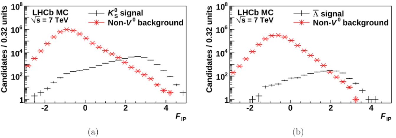
IP F -2 0 2 4 Candidates / 0.32 units 1 2 10 4 10 6 10 8 10 signal S 0 K background 0 V Non-LHCb MC = 7 TeV s (a) IP F -2 0 2 4 Candidates / 0.32 units 1 2 10 4 10 6 10 8 10 signal Λ background 0 V Non-LHCb MC = 7 TeV s (b)
Figure 1: The Fisher discriminant FIP in 0.5 million Monte Carlo simulated minimum bias events
at √s = 7 TeV for(a)K0
S and (b)Λ.
daughter tracks to be reconstructed through the full spectrometer. Any oppositely-charged pair is kept as a potential V0candidate if it forms a vertex with χ2 < 9 (with one degree of
freedom for a V0vertex). Λ, Λ and K0
S candidates are required to have invariant masses within
±50 MeV/c2 of the PDG values [14]. This mass window is large compared to the measured mass resolutions of about 2 MeV/c2 for Λ (Λ) and 5 MeV/c2 for K0
S.
Combinatorial background is reduced with a Fisher discriminant based on the impact parameters (IP) of the daughter tracks (d±
) and of the reconstructed V0
mother, where the impact parameter is defined as the minimum distance of closest approach to the nearest reconstructed primary interaction vertex measured in mm. The Fisher discriminant:
FIP = a log10(d + IP/1 mm) + b log10(d − IP/1 mm) + c log10(V 0 IP/1 mm) (3)
is optimised for signal significance (S/√S + B) on simulated events after the above quality criteria. The cut value, FIP> 1, and coefficients, a = b = −c = 1, were found to be suitable
for Λ, Λ and K0
S at both collision energies (Fig. 1).
The Λ(Λ) signal significance is improved by a ±4.5 MeV/c2 veto around the PDG K0
S mass
after re-calculation of each candidate’s invariant mass with an alternative π+π−
daughter hypothesis. A similar veto to remove Λ (Λ) with a pπ−
(pπ+
) hypothesis from the K0
S sample
is not found to improve significance so is not applied.
After the above selection, V0yields are estimated from data and simulation by fits to the
invariant mass distributions, examples of which are shown in Fig. 2. These fits are carried out with the method of unbinned extended maximum likelihood and are parametrised by a double Gaussian signal peak (with a common mean) over a linear background. The mean values show a small, but statistically significant, deviation from the known K0
S and Λ (Λ)
masses [14], reflecting the status of the momentum-scale calibration of the experiment. The width of the peak is computed as the quadratic average of the two Gaussian widths, weighted by their signal fractions. This width is found to be constant as a function of pT and increases
linearly toward higher y, e.g. by 1.4 (0.8) MeV/c2
per unit rapidity for K0
S (Λ and Λ) at
√
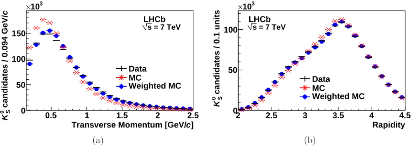
s = 7 TeV. The resulting signal yields are listed in Table 1. Significant differences are observed between V0
kinematic variables reconstructed in data and in the simulation used for efficiency determination. These differences can produce a bias
]
2
c Invariant Mass [MeV/
+ π p 1100 1110 1120 1130 2 c Candidates / 0.6 MeV/ 100 200 300 ] 2 c Invariant Mass [MeV/
+ π p 1100 1110 1120 1130 2 c Candidates / 0.6 MeV/ 100 200 300 2 c 0.03 MeV/ ± = 1115.75 µ 2 c 0.33 MeV/ ± = 1.23 σ 36 ± N = 1177 LHCb = 0.9 TeV s (a) ] 2 c Invariant Mass [MeV/
− π + π 460 480 500 520 540 2 c Candidates / 1.7 MeV/ 0 200 400 600 ] 2 c Invariant Mass [MeV/
− π + π 460 480 500 520 540 2 c Candidates / 1.7 MeV/ 0 200 400 600 µ = 496.92 ± 0.09 MeV/c 2 2 c 1.19 MeV/ ± = 5.03 σ 63 ± N = 3083 LHCb = 0.9 TeV s (b)
Figure 2:Invariant mass peaks for (a)Λ in the range 0.25 < pT < 2.50 GeV/c & 2.5 < y < 3.0 and
(b)K0
S in the range 0.65 < pT< 1.00 GeV/c & 3.5 < y < 4.0 at
√s = 0.9 TeV with field up. Signal
yields, N , are found from fits (solid curves) with a double Gaussian peak with common mean, µ, over a linear background (dashed lines). The width, σ, is computed as the quadratic average of the two Gaussian widths weighted by their signal fractions.
Table 1: Integrated signal yields extracted by fits to the invariant mass distributions of selected
V0candidates from data taken with magnetic field up and down at √s = 0.9 and 7 TeV.
√
s 0.9 TeV 7 TeV
Magnetic field Up Down Up Down
Λ 3, 440 ± 60 4, 100 ± 70 258, 930 ± 640 132, 550 ± 460
Λ 4, 880 ± 80 5, 420 ± 80 294, 010 ± 680 141, 860 ± 460
K0
S 35, 790 ± 200 40, 230 ± 220 2, 737, 090 ± 1, 940 1, 365, 990 ± 1, 370
for the measurement of Λ/K0
S given the different production kinematics of the baryon and
meson. Simulated V0
candidates are therefore weighted to match the two-dimensional pT, y
distributions observed in data. These distributions are shown projected along both axes in Fig. 3. The V0
signal yield pT, y distributions are estimated from selected data and Monte
Carlo candidates using sideband subtraction. Two-dimensional fits, linear in both pT and y,
are made to the ratios data/MC of these yields independently for Λ, Λ and K0
S, for each
magnet polarity and collision energy. The resulting functions are used to weight generated and selected V0
candidates in the Monte Carlo simulation. These weights vary across the measured pT, y range between 0.4 and 2.1, with typical values between 0.8 and 1.2.
The measured ratios are presented in three complementary binning schemes: projections over the full pT range, the full y range, and a coarser two-dimensional binning. The rapidity
range 2.0 < y < 4.0 (4.5) is split into 0.5-unit bins, while six bins in pT are chosen to
ap-proximately equalise signal V0
statistics in data over the range 0.25 (0.15) < pT < 2.50 GeV/c
from collisions at√s = 0.9 (7) TeV. The two-dimensional binning combines pairs of pT bins.
] c Transverse Momentum [GeV/
0.5 1 1.5 2 2.5 c candidates / 0.094 GeV/S 0 K 0 50 100 150 3 10 × Data MC Weighted MC LHCb = 7 TeV s (a) Rapidity 2 2.5 3 3.5 4 4.5 candidates / 0.1 unitsS 0 K 0 50 100 3 10 × Data MC Weighted MC LHCb = 7 TeV s (b)
Figure 3:(a)Transverse momentum and(b)rapidity distributions for K0
S in data and Monte Carlo
simulation at√s = 7 TeV. The difference between data and Monte Carlo is reduced by weighting
the simulated candidates.
The efficiency for selecting prompt V0decays is estimated from simulation as
ε = N(V 0 → d+d− )Observed N(pp → V0X) Generated , (4)
where the denominator is the number of prompt V0
hadrons generated in a given pT, y
region after weighting and the numerator is the number of those weighted candidates found from the selection and fitting procedure described above. The efficiency therefore accounts for decays via other channels and losses from interactions with the detector material. Prompt V0
hadrons are defined in Monte Carlo simulation by the cumulative lifetimes of their ancestors
n X i=1 cτi < 10 −9 m, (5)
where τi is the proper decay time of the ith ancestor. This veto is defined such as to keep
only V0hadrons created either directly from the pp collisions or from the strong or
electro-magnetic decays of particles produced at those collisions, removing V0
hadrons generated from material interactions and weak decays. The Fisher discriminant FIP strongly favours
prompt V0 hadrons, however a small non-prompt contamination in data would lead to a
systematic bias in the ratios. The fractional contamination of selected events is determined from simulation to be 2 − 6 % for Λ and Λ, depending on the measurement bin, and about 1 % for K0
S. This effect is dominated by weak decays rather than material interactions. The
resulting absolute corrections to the ratios Λ/Λ and Λ/K0
S are approximately 0.01.
4
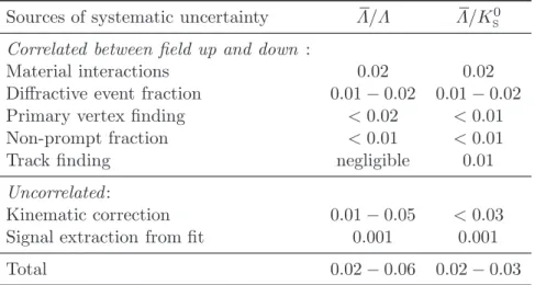
Systematic uncertainties
The measured efficiency corrected ratios Λ/Λ and Λ/K0
S are subsequently corrected for
non-prompt contamination as found from Monte Carlo simulation and defined by Eq. 5. This procedure relies on simulation and the corrections may be biased by the choice of the LHCb
] 0 X Material traversed [ 0.00 0.05 0.10 0.15 0.20 MC ) Λ / Λ / ( Data ) Λ / Λ ( 0 1 2 3 /ndf = 3.4/9.0 2 χ P = 0.9462 LHCb = 0.9 TeV s (a) ] 0 X Material traversed [ 0.00 0.05 0.10 0.15 0.20 MC )S 0 K/ Λ / ( Data )S 0 K/ Λ ( 0 2 4 6 /ndf = 9.9/9.0 2 χ P = 0.3583 LHCb = 0.9 TeV s (b)
Figure 4:The double ratios(a)(Λ/Λ)Data/(Λ/Λ)MC and (b)(Λ/KS0)Data/(Λ/K
0
S)MC are shown as
a function of the material traversed, in units of radiation length. Flat line fits, shown together with
their respective χ2 probabilities, give no evidence of a bias.
MC generator tune. To estimate a systematic uncertainty on the correction for non-prompt V0
, the contaminant fractions are also calculated using two alternative tunes of Pythia 6: Perugia 0 and Perugia NOCR [11]. The maximum differences in non-prompt fraction across the measurement range and at both energies are < 1 % for each V0species. The resulting
absolute uncertainties on the ratios are < 0.01.
The efficiency of primary vertex reconstruction may introduce a bias on the measured ratios if the detector occupancy is different for events containing K0
S, Λ or Λ. This efficiency
is compared in data and simulation using V0
samples obtained with an alternative selection not requiring a primary vertex. Instead, the V0
flight vector is extrapolated towards the beam axis to find the point of closest approach. The z coordinate of this point is used to define a pseudo-vertex, with x = y = 0. Candidates are kept if the impact parameters of their daughter tracks to this pseudo-vertex are > 0.2 mm. There is a large overlap of signal candidates with the standard selection. The primary vertex finding efficiency is then explored by taking the ratio of these selected events which do or do not have a standard primary vertex. Calculated in bins of pT and y, this efficiency agrees between data and simulation to better
than 2 % at both √s = 0.9 and 7 TeV. The resulting absolute uncertainties on Λ/Λ and Λ/K0
S are < 0.02 and < 0.01, respectively.
The primary vertex finding algorithm requires at least three reconstructed tracks.3
There-fore, the reconstruction highly favours non-diffractive events due to the relatively low effi-ciency for finding diffractive interaction vertices, which tend to produce fewer tracks. In the LHCb MC simulation, the diffractive cross-section accounts for 28 (25) % of the to-tal minimum-bias cross-section of 65 (91) mb at 0.9 (7) TeV [6]. Due to the primary vertex requirement, only about 3 % of the V0
candidates selected in simulation are produced in diffractive events. These fractions are determined using Pythia 6 which models only soft diffraction. As a cross check, the fractions are also calculated with Pythia 8 which includes
3
The minimum requirements for primary vertex reconstruction at LHCb can be approximated in Monte Carlo simulation by a generator-level cut requiring at least three charged particles from the collision with lifetime cτ > 10−9m, momentum p > 0.3 GeV/c and polar angle 15 < θ < 460 mrad.
Table 2: Absolute systematic errors are listed in descending order of importance. Ranges indicate uncertainties that vary across the measurement bins and/or by collision energy. Correlated sources of uncertainty between field up and down are identified.
Sources of systematic uncertainty Λ/Λ Λ/K0
S
Correlated between field up and down :
Material interactions 0.02 0.02
Diffractive event fraction 0.01 − 0.02 0.01 − 0.02
Primary vertex finding < 0.02 < 0.01
Non-prompt fraction < 0.01 < 0.01
Track finding negligible 0.01
Uncorrelated:
Kinematic correction 0.01 − 0.05 < 0.03
Signal extraction from fit 0.001 0.001
Total 0.02 − 0.06 0.02 − 0.03
both soft and hard diffraction. The variation on the overall efficiency between models is about 2 % for both ratios at√s = 7 TeV and close to 1 % at 0.9 TeV. Indeed, complete removal of diffractive events only produces a change of 0.01 − 0.02 in the ratios across the measurement range.
The track reconstruction efficiency depends on particle momentum. In particular, the tracking efficiency varies rapidly with momentum for tracks below 5 GeV/c. Any bias is expected to be negligible for the ratio Λ/Λ but can be larger for Λ/K0
S due to the different
kinematics. Two complementary procedures are employed to check this efficiency. First, track segments are reconstructed in the tracking stations upstream of the magnet. These track segments are then paired with the standard tracks reconstructed through the full detector and the pairs are required to form a K0
S to ensure only genuine tracks are considered. This
track matching gives a measure of the tracking efficiency for the upstream tracking systems. The second procedure uses the downstream stations to reconstruct track segments, which are similarly paired with standard tracks to measure the efficiency of the downstream tracking stations. The agreement between these efficiencies in data and simulation is better than 5 %. To estimate the resulting uncertainty on Λ/Λ and Λ/K0
S, both ratios are re-calculated after
weighting V0
candidates by 95 % for each daughter track with momentum below 5 GeV/c. The resulting systematic shifts in the ratios are < 0.01.
Particle interactions within the detector are simulated using the Geant 4 package, which implements interaction cross-sections for each particle according to the LHEP physics list [10]. These simulated cross-sections have been tested in the LHCb framework and are consistent with the LHEP values. The small measured differences are propagated to Λ/Λ and Λ/K0
S to estimate absolute uncertainties on the ratios of about 0.02. V
0
absorption is limited by the requirement that each V0
decay occurs within the most upstream tracker (the VELO). Secondary V0production in material is suppressed by the Fisher discriminant,
which rejects V0
candidates with large impact parameter. The potential bias on the ratios is explored by measurement of both Λ/Λ and Λ/K0
(deter-mined by the detector simulation), in units of radiation length, X0. Data and simulation are
compared by their ratio, shown in Fig.4. These double ratios are consistent with a flat line as a function of X0, therefore any possible imperfections in the description of the detector
material in simulation do not have a large effect on the V0
ratios. Note that the double ratios are not expected to be unity since simulations do not predict the same values for Λ/Λ and Λ/K0
S as are observed in data.
The potential bias from the Fisher discriminant, FIP, is investigated using a pre-selected
sample, with only the track and vertex quality cuts applied. The distributions of FIP for Λ,
Λ and K0
S in data and Monte Carlo simulation are estimated using sideband subtraction.
The double ratios of data/MC efficiencies are seen to be independent of the discriminant, implying that the distribution is well modelled in the simulation. No systematic uncertainty is assigned to this selection requirement.
A degradation is observed of the reconstructed impact parameter resolution in data com-pared to simulation. The simulated V0 impact parameters are recalculated with smeared
primary and secondary vertex positions to match the resolution measured in data. There is a negligible effect on the V0ratio results.
A good estimate of the reconstructed yields and their uncertainties in both data and simulation is provided by the fitting procedure but there may be a residual systematic un-certainty from the choice of this method. Comparisons are made using side-band subtraction and the resulting V0yields are in agreement with the results of the fits at the 0.1 % level.
The resulting absolute uncertainties on the ratios are on the order of 0.001. Simulated events are weighted to improve agreement between simulated V0
kinematic distributions and data. As described in Section 3, these weights are calculated from a two-dimensional fit, linear in both pTand y, to the distribution of the ratio between reconstructed
data and simulated Monte Carlo candidates. This choice of parametrisation could be a source of systematic uncertainty, therefore alternative procedures are investigated including a two-dimensional polynomial fit to 3rd
order in both pT and y and a (non-parametric) bilinear
interpolation. The results from each method are compared across the measurement range to estimate typical systematic uncertainties of 0.01 − 0.05 for Λ/Λ and < 0.03 for Λ/K0
S.
The lifetime distributions of reconstructed and selected V0
candidates are consistent between data and simulation. The possible influence of transverse Λ (Λ) polarisation was explored by simulations with extreme values of polarisation and found to produce no signif-icant effect on the measured ratios. Potential acceptance effects were checked as a function of azimuthal angle, with no evidence of systematic bias. The potential sources of systematic uncertainty or bias are summarised in Table 2.
5
Results
The Λ/Λ and Λ/K0
S production ratios are measured independently for each magnetic field
polarity. These measurements show good consistency after correction for detector acceptance. Bin-by-bin comparisons in the two-dimensional binning scheme give χ2
probabilities for Λ/Λ (Λ/K0
S) of 3 (18) % at
√
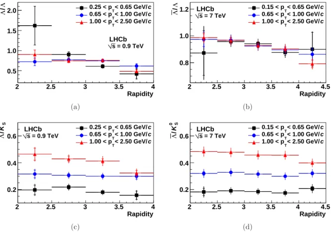
s = 0.9 TeV and 19 (97) % at √s = 7 TeV, with 12 (15) degrees of freedom. The field up and down results are therefore combined to maximise statistical significance. A weighted average is computed such that the result has minimal variance while
Rapidity 2 2.5 3 3.5 4 Λ / Λ 0.5 1.0 1.5 2.0 0.25 < pT< 0.65 GeV/c c < 1.00 GeV/ T 0.65 < p c < 2.50 GeV/ T 1.00 < p LHCb = 0.9 TeV s (a) Rapidity 2 2.5 3 3.5 4 4.5 Λ / Λ 0.8 1.0 1.2 0.15 < pT< 0.65 GeV/c c < 1.00 GeV/ T 0.65 < p c < 2.50 GeV/ T 1.00 < p LHCb = 7 TeV s (b) Rapidity 2 2.5 3 3.5 4 S 0 K/ Λ 0.2 0.4 0.6 c < 0.65 GeV/ T 0.25 < p c < 1.00 GeV/ T 0.65 < p c < 2.50 GeV/ T 1.00 < p LHCb = 0.9 TeV s (c) Rapidity 2 2.5 3 3.5 4 4.5 S 0 K/ Λ 0.2 0.4 0.6 c < 0.65 GeV/ T 0.15 < p c < 1.00 GeV/ T 0.65 < p c < 2.50 GeV/ T 1.00 < p LHCb = 7 TeV s (d)
Figure 5: The ratios Λ/Λ and Λ/KS0 from the full analysis procedure at (a) & (c)
√
s = 0.9 TeV
and (b) & (d) 7 TeV are shown as a function of rapidity, compared across intervals of transverse
momentum. Vertical lines show the combined statistical and systematic uncertainties and the short horizontal bars (where visible) show the statistical component.
taking into account the correlations between sources of systematic uncertainty identified in Table2. These combined results are shown as a function of y in three intervals of pT in Fig.5
at√s = 0.9 TeV and 7 TeV. The ratio Λ/K0
S shows a strong pT dependence.
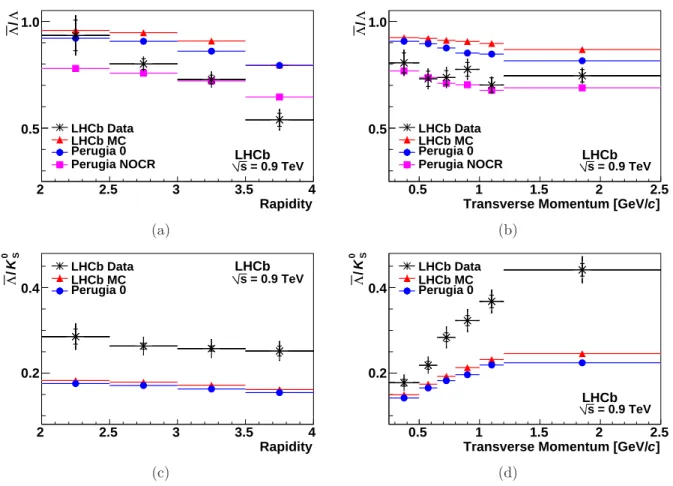
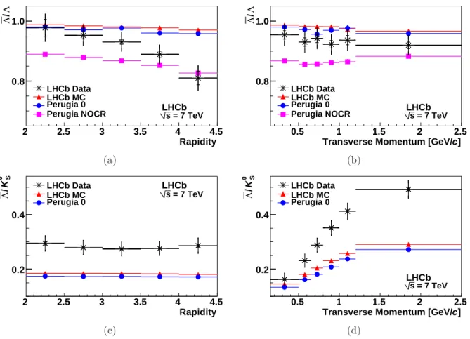
Both measured ratios are compared to the predictions of the Pythia 6 generator tunes: LHCb MC, Perugia 0 and Perugia NOCR, as functions of pT and y at √s = 0.9 TeV (Fig. 6)
and at √s = 7 TeV (Fig. 7). According to Monte Carlo studies, as discussed in Section 4, the requirement for a reconstructed primary vertex results in only a small contribution from diffractive events to the selected V0
sample, therefore non-diffractive simulated events are used for these comparisons. The predictions of LHCb MC and Perugia 0 are similar throughout. The ratio Λ/Λ is close to Perugia 0 at low y but becomes smaller with higher rapidity, approaching Perugia NOCR. In collisions at√s = 7 TeV, this ratio is consistent with Perugia 0 across the measured pT range but is closer to Perugia NOCR at√s = 0.9 TeV. The
production ratio Λ/K0
S is larger in data than predicted by Perugia 0 at both collision energies
and in all measurement bins, with the most significant differences observed at high pT.
To compare results at both collision energies, and to probe scaling violation, both pro-duction ratios are shown as a function of rapidity loss, ∆y = ybeam− y, in Fig. 8, where
Rapidity 2 2.5 3 3.5 4 Λ / Λ 0.5 1.0 LHCb Data LHCb MC Perugia 0
Perugia NOCR LHCbs = 0.9 TeV
(a)
] c Transverse Momentum [GeV/
0.5 1 1.5 2 2.5 10 × Λ / Λ 0.5 1.0 LHCb Data LHCb MC Perugia 0
Perugia NOCR LHCbs = 0.9 TeV
(b) Rapidity 2 2.5 3 3.5 4 S 0 K/ Λ 0.2 0.4 LHCb Data LHCb MC Perugia 0 LHCb = 0.9 TeV s (c) ] c Transverse Momentum [GeV/
0.5 1 1.5 2 2.5 10 × S 0 K/ Λ 0.2 0.4 LHCb Data LHCb MC Perugia 0 LHCb = 0.9 TeV s (d)
Figure 6: The ratios Λ/Λ and Λ/KS0 at
√
s = 0.9 TeV are compared with the predictions of the
LHCb MC, Perugia 0 and Perugia NOCR as a function of(a)&(c)rapidity and(b)&(d)transverse
momentum. Vertical lines show the combined statistical and systematic uncertainties and the short horizontal bars (where visible) show the statistical component.
ybeam is the rapidity of the protons in the anti-clockwise LHC beam, which travels along the
positive z direction through the detector. Excellent agreement is observed between results at both√s = 0.9 and 7 TeV as well as with results from STAR at√s = 0.2 TeV. The measured ratios are also consistent with results published by ALICE [2] and CMS [3].
The combined field up and down results are also given in tables in Appendix A. Results without applying the model dependent non-prompt correction, as discussed in Section 3, are shown for comparison in Appendix B.
6
Conclusions
The ratio Λ/Λ is a measurement of the transport of baryon number from pp collisions to final state hadrons. There is good agreement with Perugia 0 at low rapidity which is to be expected since the past experimental results used to test this model have focused on that rapidity region. At high rapidity however, the measurements favour the extreme baryon transport model of Perugia NOCR. The measured ratio Λ/K0
S is significantly larger than
Rapidity 2 2.5 3 3.5 4 4.5 Λ / Λ 0.8 1.0 LHCb Data LHCb MC Perugia 0
Perugia NOCR LHCbs = 7 TeV
(a)
] c Transverse Momentum [GeV/
0.5 1 1.5 2 2.5 10 × Λ / Λ 0.8 1.0 LHCb Data LHCb MC Perugia 0
Perugia NOCR LHCbs = 7 TeV
(b) Rapidity 2 2.5 3 3.5 4 4.5 S 0 K/ Λ 0.2 0.4 LHCb Data LHCb MC Perugia 0 LHCb = 7 TeV s (c) ] c Transverse Momentum [GeV/
0.5 1 1.5 2 2.5 10 × S 0 K/ Λ 0.2 0.4 LHCb Data LHCb MC Perugia 0 LHCb = 7 TeV s (d)
Figure 7:The ratios Λ/Λ and Λ/K0
S at
√
s = 7 TeV compared with the predictions of the LHCb MC,
Perugia 0 and Perugia NOCR as a function of(a)&(c)rapidity and(b)&(d)transverse momentum.
Vertical lines show the combined statistical and systematic uncertainties and the short horizontal bars (where visible) show the statistical component.
Rapidity loss 3 4 5 6 7 Λ / Λ 0.5 1.0 LHCb LHCb STAR 0.9 TeV, 7 TeV, 0.2 TeV, c < 2.50 GeV/ T 0.25 < p c < 2.50 GeV/ T 0.15 < p c > 0.30 GeV/ T p LHCb (a) Rapidity loss 3 4 5 6 7 S 0 K/ Λ 0.2 0.3 LHCb LHCb STAR 0.9 TeV, 7 TeV, 0.2 TeV, c < 2.50 GeV/ T 0.25 < p c < 2.50 GeV/ T 0.15 < p c > 0.30 GeV/ T p LHCb (b)
Figure 8: The ratios (a) Λ/Λ and (b) Λ/K0
S from LHCb are compared at both
√
s = 0.9 TeV
(triangles) and 7 TeV (circles) with the published results from STAR [1] (squares) as a function
of rapidity loss, ∆y = ybeam − y. Vertical lines show the combined statistical and systematic
data than expected, particularly at higher pT. Similar results are found at both √s = 0.9
and 7 TeV.
When plotted as a function of rapidity loss, ∆y, there is excellent agreement between the measurements of both ratios at√s = 0.9 and 7 TeV as well as with STAR’s results published at 0.2 TeV. The broad coverage of the measurements in ∆y provides a unique data set, which is complementary to previous results. The V0
production ratios presented in this paper will help the development of hadronisation models to improve the predictions of Standard Model physics at the LHC which will define the baseline for new discoveries.
7
Acknowledgements
We express our gratitude to our colleagues in the CERN accelerator departments for the excellent performance of the LHC. We thank the technical and administrative staff at CERN and at the LHCb institutes, and acknowledge support from the National Agen-cies: CAPES, CNPq, FAPERJ and FINEP (Brazil); CERN; NSFC (China); CNRS/IN2P3 (France); BMBF, DFG, HGF and MPG (Germany); SFI (Ireland); INFN (Italy); FOM and NWO (Netherlands); SCSR (Poland); ANCS (Romania); MinES of Russia and Rosatom (Russia); MICINN, XUNGAL and GENCAT (Spain); SNSF and SER (Switzerland); NAS Ukraine (Ukraine); STFC (United Kingdom); NSF (USA). We also acknowledge the support received from the ERC under FP7 and the R´egion Auvergne.
8
References
[1] STAR Collaboration, B. I. Abelev et al., “Strange particle production in p + p collisions at √s = 200 GeV”, Phys. Rev. C 75 (2007) 064901.
[2] ALICE Collaboration, K. Aamodt et al., “Strange particle production in proton-proton collisions at √s = 0.9 TeV with ALICE at the LHC”, Eur. Phys. J. C 71 (2011) 1594. [3] CMS Collaboration, V. Khachatryan et al., “Strange particle production in pp
collisions at √s = 0.9 and 7 TeV”, JHEP 2011 (2011) 1–40. [4] LHCb Collaboration, R. Aaij et al., “Prompt K0
S production in pp collisions at
√s =0.9 TeV”, Phys. Lett. B 693 (2010) 69.
[5] LHCb Collaboration, R. Aaij et al., “The LHCb detector at LHC”, JINST 3 (2008) S08005.
[6] I. Belyaev et al., “Handling of the generation of primary events in Gauss, the LHCb simulation framework”, Nuclear Science Symposium Conference Record (NSS/MIC) (2010) 1155. IEEE.
[7] T. Sj¨ostrand, S. Mrenna and P. Skands, “Pythia 6.4 physics and manual”, JHEP 05 (2006) 026.
[8] D. Lange et al., “The EvtGen particle decay simulation package”, Nucl. Instrum. Meth. A 462 (2001) 152.
[9] P. Golonka and Z. Was, “Photos Monte Carlo: a precision tool for QED corrections in Z and W decays”, Eur. Phys. J. C 45 (2006) 97.
[10] S. Agostinelli et al., “Geant 4: a simulation toolkit”, Nucl. Instrum. Meth. A 506 (2003) 250.
[11] P. Skands, “Tuning Monte Carlo generators: The Perugia tunes”, Phys. Rev. D 82 (2010) 074018.
[12] T. Sj¨ostrand, S. Mrenna and P. Skands, “A brief introduction to Pythia 8.1”, Comput. Phys. Commun. 178 (2008), no. 11 852–867.
[13] S. Navin, “Diffraction in Pythia”, arXiv:1005.3894 (2010).
[14] K. Nakamura et al. (Particle Data Group), “Review of particle physics”, J. Phys. G 37 (2010) 075021.
Appendix
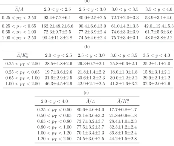
A
Tabulated results
Table 3: The production ratios Λ/Λ and Λ/K0
S, measured at
√
s = 0.9 TeV, are quoted in percent
with statistical and systematic errors as a function of (a) & (b) rapidity, y, and (c) transverse
momentum, pT[GeV/c]. (a) Λ/Λ 2.0 < y < 2.5 2.5 < y < 3.0 3.0 < y < 3.5 3.5 < y < 4.0 0.25 < pT < 2.50 93.4±7.2±6.1 80.0±2.5±2.5 72.7±2.0±3.3 53.9±3.1±4.0 0.25 < pT < 0.65 162.2±48.2±6.6 90.4±6.6±3.0 61.0±4.2±3.5 42.0±12.4±5.3 0.65 < pT < 1.00 72.3±9.7±2.5 77.2±3.9±2.4 74.6±3.3±3.9 61.7±5.6±3.6 1.00 < pT < 2.50 90.4±11.3±2.8 74.5±4.6±2.4 75.7±3.4±3.1 48.5±3.8±2.2 (b) Λ/K0 S 2.0 < y < 2.5 2.5 < y < 3.0 3.0 < y < 3.5 3.5 < y < 4.0 0.25 < pT< 2.50 28.5±1.8±2.6 26.3±0.7±2.1 25.8±0.6±2.1 25.2±1.1±2.0 0.25 < pT< 0.65 19.7±3.6±2.6 21.8±1.4±2.2 18.0±1.0±1.8 15.8±3.1±2.1 0.65 < pT< 1.00 31.6±2.9±2.5 30.6±1.3±2.3 30.0±1.2±2.2 29.9±2.1±2.2 1.00 < pT< 2.50 46.3±4.5±2.9 42.9±2.1±2.5 41.3±1.6±3.2 32.3±2.0±2.6 (c) 2.0 < y < 4.0 Λ/Λ Λ/K0 S 0.25 < pT < 0.50 80.6±4.6±4.0 17.7±0.8±1.7 0.50 < pT < 0.65 73.1±3.6±3.2 21.8±0.9±1.8 0.65 < pT < 0.80 73.7±3.2±3.7 28.4±1.0±2.3 0.80 < pT < 1.00 77.5±3.2±3.7 32.3±1.2±2.4 1.00 < pT < 1.20 70.1±3.4±2.3 36.8±1.5±2.4 1.20 < pT < 2.50 74.5±3.0±2.5 44.2±1.5±2.8
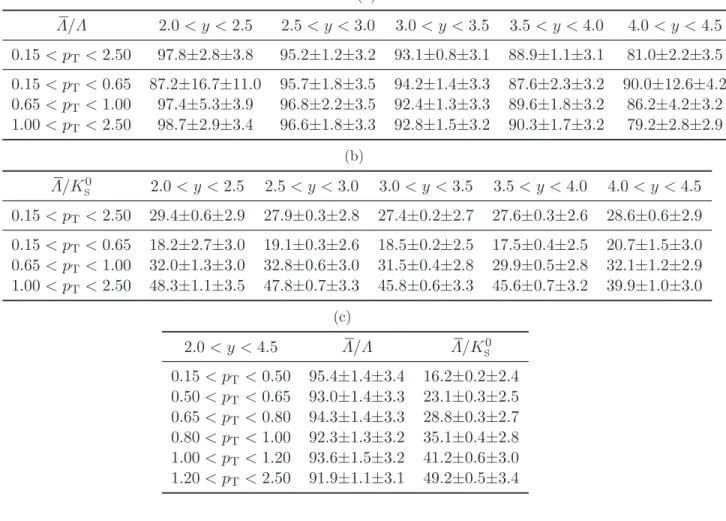
Table 4: The production ratios Λ/Λ and Λ/K0
S, measured at
√
s = 7 TeV, are quoted in percent
with statistical and systematic errors as a function of (a) & (b) rapidity, y, and (c) transverse
momentum, pT[GeV/c]. (a) Λ/Λ 2.0 < y < 2.5 2.5 < y < 3.0 3.0 < y < 3.5 3.5 < y < 4.0 4.0 < y < 4.5 0.15 < pT< 2.50 97.8±2.8±3.8 95.2±1.2±3.2 93.1±0.8±3.1 88.9±1.1±3.1 81.0±2.2±3.5 0.15 < pT< 0.65 87.2±16.7±11.0 95.7±1.8±3.5 94.2±1.4±3.3 87.6±2.3±3.2 90.0±12.6±4.2 0.65 < pT< 1.00 97.4±5.3±3.9 96.8±2.2±3.5 92.4±1.3±3.3 89.6±1.8±3.2 86.2±4.2±3.2 1.00 < pT< 2.50 98.7±2.9±3.4 96.6±1.8±3.3 92.8±1.5±3.2 90.3±1.7±3.2 79.2±2.8±2.9 (b) Λ/K0 S 2.0 < y < 2.5 2.5 < y < 3.0 3.0 < y < 3.5 3.5 < y < 4.0 4.0 < y < 4.5 0.15 < pT< 2.50 29.4±0.6±2.9 27.9±0.3±2.8 27.4±0.2±2.7 27.6±0.3±2.6 28.6±0.6±2.9 0.15 < pT< 0.65 18.2±2.7±3.0 19.1±0.3±2.6 18.5±0.2±2.5 17.5±0.4±2.5 20.7±1.5±3.0 0.65 < pT< 1.00 32.0±1.3±3.0 32.8±0.6±3.0 31.5±0.4±2.8 29.9±0.5±2.8 32.1±1.2±2.9 1.00 < pT< 2.50 48.3±1.1±3.5 47.8±0.7±3.3 45.8±0.6±3.3 45.6±0.7±3.2 39.9±1.0±3.0 (c) 2.0 < y < 4.5 Λ/Λ Λ/K0 S 0.15 < pT < 0.50 95.4±1.4±3.4 16.2±0.2±2.4 0.50 < pT < 0.65 93.0±1.4±3.3 23.1±0.3±2.5 0.65 < pT < 0.80 94.3±1.4±3.3 28.8±0.3±2.7 0.80 < pT < 1.00 92.3±1.3±3.2 35.1±0.4±2.8 1.00 < pT < 1.20 93.6±1.5±3.2 41.2±0.6±3.0 1.20 < pT < 2.50 91.9±1.1±3.1 49.2±0.5±3.4
B
Tabulated results before non-prompt correction
Table 5: The production ratios Λ/Λ and Λ/K0
S without non-prompt corrections at
√
s = 0.9 TeV
are quoted in percent with statistical and systematic errors as a function of (a)& (b) rapidity, y,
and (c)transverse momentum, pT[GeV/c].
(a) Λ/Λ 2.0 < y < 2.5 2.5 < y < 3.0 3.0 < y < 3.5 3.5 < y < 4.0 0.25 < pT < 2.50 93.1±7.2±6.0 79.3±2.5±2.4 73.2±2.0±3.2 54.1±3.1±3.9 0.25 < pT < 0.65 163.7±48.2±6.5 89.2±6.6±2.8 61.5±4.2±3.4 41.4±12.4±5.3 0.65 < pT < 1.00 71.8±9.7±2.4 76.5±3.9±2.2 75.2±3.3±3.8 62.0±5.6±3.5 1.00 < pT < 2.50 89.9±11.3±2.7 74.2±4.6±2.3 75.7±3.4±3.0 48.5±3.8±2.1 (b) Λ/K0 S 2.0 < y < 2.5 2.5 < y < 3.0 3.0 < y < 3.5 3.5 < y < 4.0 0.25 < pT< 2.50 28.9±1.8±2.4 27.2±0.7±1.9 26.6±0.6±1.9 25.6±1.1±1.8 0.25 < pT< 0.65 20.7±3.6±2.4 23.0±1.4±2.0 18.9±1.0±1.6 16.3±3.1±1.9 0.65 < pT< 1.00 31.9±2.9±2.3 31.5±1.3±2.1 31.0±1.2±2.0 30.6±2.1±2.0 1.00 < pT< 2.50 46.7±4.5±2.8 43.1±2.1±2.4 41.9±1.6±3.0 32.5±2.0±2.4 (c) 2.0 < y < 4.0 Λ/Λ Λ/KS0 0.25 < pT < 0.50 80.1±4.6±3.9 18.8±0.8±1.5 0.50 < pT < 0.65 72.9±3.6±3.1 22.9±0.9±1.6 0.65 < pT < 0.80 73.9±3.2±3.6 29.5±1.0±2.1 0.80 < pT < 1.00 77.5±3.2±3.5 33.1±1.2±2.3 1.00 < pT < 1.20 70.1±3.4±2.1 37.2±1.5±2.2 1.20 < pT < 2.50 74.4±3.0±2.3 44.5±1.5±2.6
Table 6: The production ratios Λ/Λ and Λ/K0
S without non-prompt corrections at
√
s = 7 TeV are
quoted in percent with statistical and systematic errors as a function of (a)&(b) rapidity, y, and
(c)transverse momentum, pT[GeV/c].
(a) Λ/Λ 2.0 < y < 2.5 2.5 < y < 3.0 3.0 < y < 3.5 3.5 < y < 4.0 4.0 < y < 4.5 0.15 < pT< 2.50 97.3±2.8±3.6 95.1±1.2±3.1 92.7±0.8±3.0 88.6±1.1±2.9 80.9±2.2±3.4 0.15 < pT< 0.65 85.6±16.7±11.0 95.4±1.8±3.4 93.9±1.4±3.2 87.3±2.3±3.1 90.1±12.6±4.1 0.65 < pT< 1.00 97.5±5.3±3.8 96.5±2.2±3.4 91.8±1.3±3.1 89.5±1.8±3.1 86.2±4.2±3.0 1.00 < pT< 2.50 98.2±2.9±3.3 96.6±1.8±3.2 92.5±1.5±3.1 90.0±1.7±3.1 79.0±2.8±2.8 (b) Λ/K0 S 2.0 < y < 2.5 2.5 < y < 3.0 3.0 < y < 3.5 3.5 < y < 4.0 4.0 < y < 4.5 0.15 < pT< 2.50 29.4±0.6±2.8 28.4±0.3±2.6 28.0±0.2±2.5 27.9±0.3±2.5 28.7±0.6±2.7 0.15 < pT< 0.65 18.5±2.7±2.9 20.0±0.3±2.5 19.2±0.2±2.3 17.9±0.4±2.3 21.1±1.5±2.9 0.65 < pT< 1.00 32.3±1.3±2.9 33.3±0.6±2.8 32.2±0.4±2.7 30.2±0.5±2.6 32.2±1.2±2.7 1.00 < pT< 2.50 47.9±1.1±3.3 47.5±0.7±3.2 45.7±0.6±3.2 45.6±0.7±3.1 39.5±1.0±2.8 (c) 2.0 < y < 4.5 Λ/Λ Λ/K0 S 0.15 < pT < 0.50 95.0±1.4±3.2 16.9±0.2±2.3 0.50 < pT < 0.65 92.9±1.4±3.2 23.8±0.3±2.4 0.65 < pT < 0.80 94.0±1.4±3.2 29.4±0.3±2.5 0.80 < pT < 1.00 91.9±1.3±3.1 35.5±0.4±2.7 1.00 < pT < 1.20 93.1±1.5±3.1 41.3±0.6±2.9 1.20 < pT < 2.50 91.8±1.1±3.0 48.9±0.5±3.2