Aircraft Charging Using Ion Emission for Lightning Strike
Mitigation: An Experimental Study
by
Theodore Mouratidis
Submitted to the Department of Aeronautical and Astronautical
Engineering
for the partial fulfillment of the requirements for the Degree of
Masters of Science in Aeronautical and Astronautical Engineering
at the
MASSACHUSETTS INSTITUTE OF TECHNOLOGY
Novemiber-2018 Ed
s B\0
o
Massachusetts Institute of Technology -2908.
Z-Author ...
All Rights Reserved.
Signature redacted
De
ent of Aeronautical and Astronautical Engineering
I
Signature
redacted
Certified By ..
-Certified By ...
November 28, 2018
Manuel Martinez Sanchez
Emeritus Professor
Thesis Supervisor
Signature redacted
Signature redacted
Carmen Guerra Garcia
Assistant Professor
Thesis Supervisor
Accepted By
MASSACHUSEMS INSTITUTE OF TECHNOLOGYMAR 12 2019
LIBRARIES
Sertac Karaman
Chairman, Department Committee on Graduate Theses
1
Abstract
Lighting strikes are a problem for aircraft flying in large external electric fields. In most cases, the strike is triggered by the aircraft; as it flies through an electric field, it becomes polarized, and on areas with small radius of curvature, the electric field is magnified. This can result in bi-directional leaders which extend from opposite polarity aircraft extremities. These can connect to oppositely charged regions in a cloud or the ground, resulting in a lightning strike. Current meth-ods to avoid lightning are limited to avoiding thunderstorm regions, as recommended by weather radar or conversations between pilots and the ground. Methods to treat the symptom of a strike have been relatively successful; a mesh placed under the skin of the aircraft can distribute the cur-rent and heat of the localized strike. However, there are curcur-rently no active measures to prevent the strike from happening. The Boeing Lightning Strike team at MIT has recently proposed an active system that exploits the physics of how a lightning arc is triggered from an aircraft in flight based on net charge control of the vehicle. The objective of this thesis is to prove the feasibility of controlling the net charge of an aircraft in flight by using ion emission from its surface. Differ-ent strategies to control the net charge of a flying isolated body were explored and analyzed. The first strategy tested was based on using charge emission from an electrospray source. A passive flow and forced flow configuration were tested, however it was shown that there were numerous difficulties associated with running the electrosprays in atmospheric pressure. To overcome the limitations of the electrospray source, a second strategy was tested based on a controlled corona discharge, which is known to have increasing current emission with increasing wind speed. The first experiment was setup in the Wright Brothers Wind Tunnel; sharp tips were used to generate a corona discharge and a metallic sphere was used to simulate the aircraft. Significant electrical potential saturation was observed on the sphere, and it is likely this was due to the filamentary streamer corona regime which produces both positive and negative ions. Thus a new experiment
was designed; a thin wire was used to generate a glow corona, which produces predominantly pos-itive ions, and this was attached using GlO (a fiberglass composite material) to a metallically coated airfoil. Charging of much higher magnitudes was observed, indicating the glow corona regime is critically important in optimizing the potential of the airfoil. Charge control of an air-foil (Chord 0.2 m, Span 1 m) at 40 m/s was demonstrated to a level of -42 kV. For an object of a given characteristic size, a certain amount of charge is required to satisfy the optimal charge con-dition, where negative and positive leader strikes are both equally likely or unlikely. The achieved potential of -42 kV is the order of magnitude required for this size airfoil based on the theoretical estimates, and these tests also showed a trend of linear potential variation with wind speed.
Acknowledgments
I would like to thank everybody who assisted me in any form over the last 24 months. First I
would like to thank the faculty, Professor Manuel Martinez Sanchez, Professor Paulo Lozano, Pro-fessor Carmen Guerra Garcia, and ProPro-fessor Jaime Peraire, in all their guidance and direction
-both theoretical and experimental. I would also like to thank Todd Billings and Dave Robertson
-none of the experiments would have been constructed or completed without their help. I would also like to thank my family and friends for their support while completing this work. Finally, I would like to thank the Boeing Company for financially supporting my Research Assistantship and in particular Ben Westin for supporting the group and our research.
Contents
1 Introduction 11
1.1 Aircraft Triggered Lightning . . . . 11
1.2 Atmospheric Phenomena Leading to Lightning . . . . 12
1.2.1 Charge Separation in Clouds . . . . 12
1.2.2 Lightning Propagation . . . . 14
1.3 A charge control strategy to reduce the probability of aircraft-triggered lightning . . 16
1.3.1 Pre Lightning Electrostatics and Lightning Initiation Model . . . . 16
1.4 Scope and Outline of this Thesis . . . . 19
2 Charge Control Experiments using electrosprays 20 2.1 Net Charge Control by Charge Emission . . . . 20
2.2 Electrospray Background . . . . 20
2.3 Experimental Setup . . . . 25
2.3.1 Passive Capillary Electrospray . . . . 25
2.3.2 Forced flow Configuration . . . . 27
2.4 Results and Discussion . . . . 29
2.4.1 Passive Capillary Electrospray . . . . 29
2.4.2 Forced Flow Configuration . . . . 32
3 Charge Control Experiments using Controlled Corona Discharge 34 3.1 Corona Background . . . . 34
3.1.1 What is a Corona? . . . . 34
3.1.3 Existence of the Glow Regime . . . .
3.1.4 Current from a 2D Glow Corona . . . .
3.2 Corona Discharge in Wind . . . . 3.3 Experimental Design . . . .
3.4 Building the Corona Sphere Experiment . . . .
3.5 Experimental Methods . . . . 3.5.1 Sphere Charging in Wind . . . .
3.5.2 Insulation and Communication . . . .
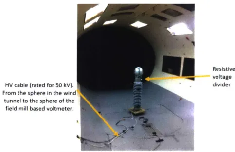
3.5.3 Diagnostics: Floating Potential Measurement .
3.6 Experimental Results and Discussion . . . .
3.6.1 Visualization of Corona Discharge . . . .
3.6.2 Charging of Sphere in WBWT facility: Prelimi
3.6.3 Unshielded Wind Tunnel Walls . . . .
3.6.4 Sphere Potential Saturation Model . . . .
3.6.5 Shielded Wind Tunnel Walls . . . . 3.6.6 Parametric analysis of charge control . . . .
3.6.7 Tips Together . . . .
3.6.8 Tips Splayed . . . .
3.6.9 Results: Plots for Splayed Tips . . . .
3.6.10 3.6.11 3.6.12
nary
Discussion: Sphere Potential Dependence on Radial Discussion: Sphere Potential Dependence on Axial
UV Camera Photography . . . . . . . . 36 . . . . 36 . . . . 38 . . . . 40 . . . . 43 . . . . 47 . . . . 47 . . . . 48 . . . . 49 . . . . 52 . . . . 52 Tests . . . . 55 . . . . 55 . . . . 56 . . . . 58 . . . . 62 . . . . 63 . . . . 65 . . . . 66 Position . . . . 69 ?osition . . . . 69 . . . . 70
4 Charge Control Experiments using Glow Corona Discharge and Airfoil Geometry 72 4.1 Experim ental Setup . . . . 72
4.1.1 Shifting to the Glow Regime . . . . 72
4.1.2 Experimental Configuration . . . . 73
4.2 Results and Discussion . . . . 74
4.2.1 Current Characterization without Wind - Corona Wire Voltage Sweep . . . . 74
4.2.2 Dependency of Current and Charging Level with Wind, Radial and Axial P osition . . . . 75
4.2.3 Comparison of the two methods to measure the electrostatic potential of the airfoil . . . . 89
4.2.4 UV photography of the corona emission . . . . 92 5 Conclusion and Future Work 93 5.1 Conclusions and Future Work . . . . 93
Nomenclature
a Townsend Ionization Coefficient (rn- 1)
C Dielectric Constant
(O Permittivity of Free Space 8.85 x 10- 1 2(m-3kg- 1s4A2)
7 Townsend Attachment Coefficient (m-1)
y
Surface Tension (N/m)te Electron mobility (m2/Vs)
Pi Ion mobility (Mr 2/Vs)
Potential Parameter Potential (V)
Ion Stream Function
OQ Ion Stream Function due to Electric Field
Ow Ion Stream Function due to Wind
a- Charge Density (C/n2
)
TH Hydrodynamic Relaxation Time (s)
0 Angle (o)
C Capacitance (F)
Do Sea Level Density (1.225(kg/m"))
E Electric Field (V/m)
e Unit Charge 1.6 x 10- 19(C)
E, Normal Electric Field (V/m)
Ep Peek Electric Field (V/m)
E+cr Positive Critical Corona Breakdown Field (V/rn)
E_c Negative Critical Corona Breakdown Field (V/m)
Ec, Critical Electric Field (V/rm)
I Current (A)
IL Surface Current (A)
K Conductivity (Si) 1 Length (m) N Number Density (M- 3) Ne Electron Density (m- 3 ) Q Charge (C)
Qv Volume Flow Rate (m3
/s)
r Radius (m)
r* Characteristic Passage Radius (m)
R1, R2 Principle Radii of Curvature (m)
T Temperature (K)
Ter Critical Temperature (K)
V Voltage (V)
Vo Corona Starting Voltage (o)
vC, Free Stream Velocity (m/s)
Vstart Electrospray starting voltage (V)
Chapter 1
Introduction
1.1
Aircraft Triggered Lightning
Our proposition is that a charge control strategy would reduce the probability of an aircraft-triggered lightning strike [7]. Ways to reduce the effects of lightning strikes have been treated before - Meshes are routinely embedded in the airframe to distribute and dissipate the current associated with the lightning strike, as well as to avoid direct burning of the strike point. They also provide a Faraday cage effect and protect the electronics inside the aircraft [3]. This method to reducing the direct effects of a lightning strike has been quite successful, however the strike itself is not avoided. A method of mitigation has been proposed and modified during the duration of this period of re-search; the proposition is not just to treat the symptom after the strike has occurred, but to pre-vent the strike all together.
Electrosprays have been intensively researched for medical and space propulsion applications. Their efficiency, thrust density, and low levels of propellant required make them an attractive source for many applications. Additionally, controlled corona discharges are also known to be effi-cient methods of current emission in high speed flows. Using one of these methods to change the equipotential surfaces around an aircraft alters the breakdown field required for a natural corona discharge to occur. Natural corona discharges that form on the aircraft can transition from glow to streamer coronas (Refer to 3.1). These can then transition to leader formation, which can eas-ily propagate and connect with a leader from a cloud, forming a lightning bolt. By biasing the aircraft surface using either an electrospray or a controlled corona discharge, the charge on an
air-craft can be controlled. This reduces the probability of a strike because the maximum electric field on the aircraft is moved further away from the critical positive and negative breakdown electric fields necessary for the strike to occur. Assuming we have the necessary amount of high voltage power supplies, then these solutions could be implemented. This thesis discusses the last two years of research regarding the most efficient methods to charge an aircraft for lightning strike mitiga-tion.
For completeness, in what follows, the charge control strategy will be summarized. More details can be found in [7]. When an aircraft is in an external electric field it becomes polarized (Figure
1.1) as the electric field is magnified at areas of small radius of curvature. These ambient electric
fields can be enough to cause corona breakdown at the aircraft extremeties. Corona breakdown can result in bi-directional leaders which can connect with oppositely charged regions in the cloud. The aircraft triggers a lightning strike - with itself being the direct path of the return current. Because of the differing physics of the positive and negative corona breakdown, E+c, = E-cr/ 2, [7] we can exploit the asymmetry in the critical breakdown fields. Here E+c, is the positive crit-ical corona breakdown electric field, and E__, is the negative critical corona breakdown electric field. In most cases, since the positive leader has a lower breakdown threshold, a positive leader develops first, shifts aircraft to negative potential as it drains current, and then negative side trig-gers a negative leader. The goal is to keep the positive side sub critical, and doing so carefully so that the negative side will still be far from critical; this can be done by reducing the potential of the aircraft through the emission of positive ions.
1.2
Atmospheric Phenomena Leading to Lightning
1.2.1
Charge Separation in Clouds
Before we speak of lightning, it is important to introduce the definitions of streamers and sparks; these will be spoken of further in section 3.1, 'Corona Background'. A streamer is a filamentary corona discharge which occurs on the electrodes with very small radius of curvature where the electric field is at least 1.8 times greater than breakdown of air. A spark is caused by the complete electrical breakdown of air; it is plasma channel formed in a normally insulating medium. Now, following streamer formation, the probability of a spark discharge becomes very high. Lightning is a large scale spark discharge. Much of the physics of the formation of lightning and its
prop-WHAT TRIGOER LIGHINING: . flykng vicar etectiKAbly charged dAdt.he
espnmiatly during taklog oe landing,
a pLlne can trigger a bolta n.atng
Ughumag is the d(C.ge uudden A s i
of electrcty between negatily tw posit lycharged areas
"Rehin ouhds and trom
douds to ground q
The aahtniiw baft (Atstrikt the
airplane, nmeos along de exterior
of the plane () atd t lts to tes
l c d ed (Q. Datcge is
On average, eah coimucMa
airplane Is struck by lightning
tcolee a Yeare Often It's the
presence of the airplane that
triggers a lghtning bolt
Figure 1.1: Aircraft being struck by Lightning [6]
agation is poorly understood, but there have been numerous models developed to provide some insight into the complex processes at hand.
Within a cloud, ionization due to cosmic rays, or decay of water molecules due to collisions can
lead to charged particles. Negative charges collect at the bottom of the cloud, and positive charges collect at the top of the cloud. To understand how this occurs we need to look more closely at the chemistry of the water molecules.
Water molecules are polar in nature, and arrange themselves with the positive ends facing inward
from the water surface. Therefore a double electric layer forms on the surface of the droplet, with a voltage drop experimentally determined as A0 = 0.26 V [4]. Negative ions are trapped near the
drop[4]:
N ~ 47rcor(
e
Where r is the droplet radius, N is the number density of ions, EO is the permittivity of free space, and e is the electronic charge. This equation is determined from the fact that a droplet of a given radius is able to absorb a specific number of ions: for a droplet of radius r = 10pm, it is able to absorb 2000 negative ions. Thus these heavier droplets now descend to the bottom of the cloud, while the positive ions remain in molecular form at the top parts of the cloud. This phenomenon is what creates the charge distribution in a cloud and leads to lightning discharges within them.
1.2.2
Lightning Propagation
There exists triggered lightning and natural lightning [16]. This brief section will describe the pro-cess of natural lightning (not specific to aircraft). Each lightning strike begins with the formation and propagation of a leader channel. These are called multi-step leaders and have relatively low current, length and velocity. As these leaders approach the Earth, the electric field between the propagating front and the Earth increases such that a formation of a very strong ionization wave
is created, moving backward in the direction of the thundercloud. This is called the 'back ioniza-tion wave' or the 'return stroke'. This is main part of the lightning discharge. The velocity of the return stroke reaches up to 0.3 of the speed of light, and up to 100 kA. The temperature in the channel reaches 25,000 K with electron densities of 1 - 5 x 10'7cm3
[4], which implies complete ionization. The front of this return stroke has a large electric field, with intensive ionization, cre-ating a plasma channel with high enough conductivity to form a channel of the spark. The rapid heat release leads to strong pressure increases in the plasma channel of a lightning discharge and therefore to a shock wave which is heard as thunder. As this return stroke propagates through the initial leader channel, a fully developed spark channel forms. The attachment process between the downward negative leader and the upward positive streamer is very complex and not yet fully physically determined. Figure 1.2 shows the described process.
++~V
+ ++ + ++ I MI Gnu 1.2m +F+ -A chmn -20.00 ams 2010"m 0 .0 80b0ody.0 s 19.00 .3 20.20 ms -Sooond Wm 62.05 rm1.3
A charge control strategy to reduce the probability of
aircraft-triggered lightning
This section will detail the theory behind the mission to mitigate lightning strikes. 90% of aircraft lightning strikes are triggered by the vehicle itself. A bi directional leader precedes the damaging strike. There is an asymmetry in the breakdown fields; positive breakdown is about 50% of the negative breakdown value. The hypothesis of this project is that the optimal aircraft charge con-dition, is when both the positive and negative leaders are equally unlikely.
The invention of the team is an active system to reduce the risk of a strike [10], [12]. First, sen-sors will be used to determine the external field and net charge. Secondly, a control system will be activated in which the net charge of the aircraft will be altered using ion emitters to drive the net charge of the aircraft to its optimal level.
1.3.1
Pre Lightning Electrostatics and Lightning Initiation Model
Electric field amplification
Leader inception
E aJ -oEndS Outputs
-
Attachment pointsE,/ 9-oE. A Threshold ambient fields
Figure 1.3: Pathway for leader inception threshold determination [8]
Figure 1.3 shows how the electric field on the aircraft surface and its vicinity is amplified, lead-ing to a corona and leader inception. Dependlead-ing upon the polarization of the aircraft, the elec-tric field can be enhanced in certain ways. The elecelec-tric field amplification also depends on the net charge and orientation of the electric field. The local amplification of the electric field can lead to electron avalanches. Electron multiplication is dictated by the inequality
a
- rj > 0, which isdirectly present in the electron production equation:
dNe = - -+ N, = e b--) (1.2)
Where a is the Townsend ionization coefficient, r1 is the Townsend attachment (recombination) coefficient and N, is the electron density. From Gallimberti 1979 [5], 'Leader inception occurs when T > Te,. For T > Tc, detachment of electrons from 02 supplies the discharge with copious
amounts of electrons, enhancing conductivity, ionization, and further raising the gas temperature." Here T is the gas temperature and Tc, is the critical gas temperature where leader inception oc-curs. This temperature criterion can be translated into a corona charge accumulation criterion (Figure 1.3). What we can see from the optimum charge level displayed in Figure 1.4 (positive and negative leader inception equally likely), is that the aircraft can fly in a much higher electric field (about 50% higher)[8].
We could imagine an experimental scenario or a real scenario for that matter of an aircraft in an ambient electric field. As stated, of interest is the optimal charge configuration so as to maxi-mize the ambient field required to trigger lightning arc inception. Some computational work for a 1/18th scale model Falcon by Ngoc Cuong, who is part of the Lightning Strike Research team, is shown in the table Figure 1.4. If we now go ahead and plot these results in Figure 1.5, we can see clearly that there is an optimal charge configuration for the aircraft; this corresponds to a po-tential, and gives information about the critical breakdown voltage or electric field for that sce-nario. Indeed it is estimated that the critical breakdown field is 50% higher than in the uncharged case[7]. In Figures 1.4 and 1.5, Vapp is an applied potential in an experimental scenario simulating the external ambient electric field,
Q
is the charge of the aircraft, and Ou is the potential of the aircraft due to charging.The charge and potential magnitudes have various scalings with size and other parameters and it is informative to investigate these scalings. The most important scaling is as follows[8]:
Q Oc l2coE, (1.3)
Where 1 is a length scale, and E, is the normal electric field. This can give us estimates of the optimal charge condition for our experimental scenarios when we attempt to charge up a floating body, corresponding to some potential for a given characteristic size.
Q [pC] Om [kV] 0 0 (+)V stab. (-)Nose 970 15.4 -2 -43 (+)V stab. (-)Nose 1122 11.4 4 -4 -85 (+) V stab. (-) Nose 1274 7.4 -6 -128 (+)V stab. (-)Nose 1426 2.9 -7 -149 (+)V stab. (-) Nose 1510 0.6 -8 -170 (-) Nose -10 -213 (-)Nose -12 -255 (-) Nose
*Fixed orientation (vertical field) Figure 1.4: 1/18 Scale Falcon Model ble [8] (+) V stab. (+) V stab. (+) V stab. 1392 953 297 2.4 9.5 16.2
- Lightning Arc Inception as
I" leader
o.
.... ..... 0 0o
-t Estimated increase of 50% in0 the breakdown votage compared to uncharged case
--
TOO
-250 -200 -150 -100 -50 0<1I [kV]
Figure 1.5: 1/18 Scale Falcon
[8]
Model - Lightning Arc Inception as a Function of Net Charge - Plot
160 140 120 100 80 60 40 20
2'd leader Vapp [kV ] Ilit [c n]
Q = -7pC
Positively charged Negatively charged
Ta-1.4
Scope and Outline of this Thesis
The objectives of this campaign were to investigate various methods for charge control strategies to prevent lightning strikes on aircraft, by charging a metallic object to the optimum value for its size, such that the positive and negative critical breakdown fields are equally unlikely. This thesis covers three major experimental campaigns to prove on a smaller scale, that this objective was feasible. The first effort involved the use of electrosprays, the second used streamer coronas and the third used a glow corona. Only the corona efforts were tested in high speed flows because the electrosprays were shown to be difficult to operate in atmosphere, let alone in a high speed flow. The streamer corona was tested using a sphere to represent the aircraft, as the preliminary theoretical studies were simple in this configuration, and experimentally, storing the equipment was easier. The glow corona on the airfoil geometry was shown to be the most successful method for charging. All of the experimental work done for each of these campaigns is presented in this thesis, and the optimal configurations for maximal charging efficiency are shown. The next stage following this campaign should be the implementation of the glow corona on a UAV.
Chapter 2
Charge Control Experiments using
electrosprays
2.1
Net Charge Control by Charge Emission
The way to adjust the charge, and therefore potential and electric field of the aircraft is done using a charge emitting device. In our case, we have a device (electrospray or corona discharge) which emits positive ions. The charge emitting device is biased at a fixed potential relative to the aircraft. As the ion emitter emits positive charges, the potential of the whole system, aircraft and emitter, becomes negatively charged; This is how the potential of the aircraft is reduced.
2.2
Electrospray Background
Electrosprays were a monumental discovery for a variety of applications, particularly micro propul-sion for use in spacecraft. The basic principle on which they operate is by application of a poten-tial difference between the operating liquid and an extractor plate. They can work in the pure droplet, pure ionic or mixed droplet-ion regime. For propulsion application, the usage of an ex-ternal power supply eliminates the constraint of chemical energy stored in the bonds of liquid or solid propellants. Of course the weight of. the power supply poses other restrictions, however it essentially allows for extremely high exhaust velocities and therefore specific impulses. This
in turn means a very highly efficient usage of propellant or liquid. Additionally the flexibility of operating in different regimes means we can choose a particular m/q mass to charge ratio. For some given exhaust speed we can choose a lower mass to charge ratio, or higher charge to mass ra-tio (ionic regime) to lower the required accelerating voltage. For our applicara-tion, we do not care about 'thrust' levels but of course there would be a trade off between lowering the accelerating voltage and increasing the mass to charge ratio to increase the thrust density, and thus the total current or charge emitted. The thrust density and specific impulses achievable make electrosprays very attractive micro propulsion sources.
Now to speak of the physics of electrospray propulsion. In the capillary configuration, the electric field at the liquid meniscus will form a Taylor cone. The normal electric field will mathematically become infinite at the cone tip. Physically this is overcome by liquid emission of droplets and or ions at the tip. Let us proceed through the mathematical formulation of the electrospray physics. First we can come up with an expression for the normal electric field on the Taylor Cone surface. Assuming that initially there is no tip emission and the free charges within the liquid are fully re-laxed on the surface due to the electric field, then there is no internal electric field Ej = 0. Now there is a simple balance of electrostatic and surface tension forces on the tip of the cone
menis-cus[11]:
-coE2 (11)+(2.1)
2 R1 R2
Where R1 and R2 are the two principal radii of curvature of the cone meniscus. The radius of
cur-vature along the cone length is R1 = oc because it has no curvature. The second principal radius of curvature of the cone in the azimuthal direction can be calculated using Meusnier's theorem
-R2 = r/ tan(O).
Thus the expression for the normal electric field can be written as[11]:
E, = 2' cot( ) (2.2)
r6o
In 1964 Sir Geoffrey Ingram Taylor [17] derived the shape of this cone, in particular he went about calculating the angle of the cone. In addition to the assumption that the cone exists in a steady
state equilibrium and at zero differential pressure with respect to the outside gas, it was assumed that the surface of the Taylor Cone was an equipotential. Then Laplace's equation can be solved in the region outside the cone. For the specified geometry, admits the solutions
#
= Q,(cos(0))r",and q = P,(cos(0))r". P and
Q
are the Legendre Polynomials of the first and second kind. The Legendre polynomial of the second kind is appropriate for the Taylor cone because it has a singularity at 0 = 0 which is inside the cone, and we only require the solution outside of theTay-lor cone. To find the normal electric field we use the 0 derivative in polar coordinates[11]:
108# dQ
E, = Eo - 0 :r"-1 sin(O) "Q (2.3)
r 00 d(cos())
For this expression to match up the previously calculated expression for the normal electric field, we require that v = 1/2. Therefore the potential solution becomes:
0 = 0 + QI/2(cos(0))r1/2 (2.4)
Since the potential is directly proportional to the radius r, then the potential will vary everywhere unless there is some angle 0 which sets the whole term to zero, such that the Taylor Cone surface is an equipotential. After we solve the Legendre term to zero, it is found that the Taylor Cone angle is 49.230.
Further analysis can be done to determine the current emitted and some of the physical param-eters of the cone jet. Juan Fernandez De La Mora [2] first came up with the formula for the cur-rent emitted from a Taylor cone jet operating in the pure droplet mode. (The pure ionic mode current and characteristic parameters are analyzed slightly differently).
Let us introduce the hydrodynamic relaxation time of charges to the surface of a conductive liq-uid. If an electric field is applied to the gas next to a liquid surface, the charges will collect on the surface at a rate:
do-do = KE,
(2.5)
dt
Where
o-
is the free charge density, K is the conductivity of the liquid, and Ei is the internal elec-tric field in the liquid. From Gauss' law, namely V- D = p, the free charge density at the surfacecan be related through the internal and external electric fields:
6EOE - ccoEi = a (2.6)
Where EO is the external electric field. Thus we can form a differential equation for the charge density:
do- K K
-+ - - Eo (2.7)
dt Eco 6
Solving this differential equation, we have:
o- =
oE(1
- e-t/r) (2.8)Thus the hydrodynamic relaxation time is TH
-In operation of the electrospray, the tip of the Taylor cone breaks up into the jet. We can define a characteristic passage time, Tp = ! [2], which is the time which particles spend in the transition
from cone to jet region. When this becomes approximately equal to the hydrodynamic relaxation time, we know the tip has broken up and is not an equipotential anymore. This leads to the char-acteristic passage radius r* = (oQ )1/3. We assume the current is fully convected on the surface of the Taylor Cone. The current can be written as[11]:
I, = 27r sin(O)r*au (2.9)
Where I is the surface current, and u is the flow velocity. For mathematical simplicity, we will assume that the charges are still fully relaxed, so that we.have a simple expression for the surface
charge - = cEO. The velocity can also be written as:
U = Qv (2.10)
27rr*2(1 - cos(O))
After substitution into the original equation for the current we arrive at the following equation [2]:
Iu = f(c)
f
(2.11)experimen-tally). Now, this factor is about 3 theoretically using the Taylor cone angle, but this is not accu-rate because we had to assume full charge relaxation in this calculation, and this is clearly not what happens at the tip of the Taylor Cone. There are three important points to take from this equation. Firstly, the current is independent of the electrode shape. Secondly, the current is inde-pendent of the fluid viscosity. Thirdly, the current is indeinde-pendent of the applied voltage, however this is only true if, as Taylor assumed, the internal pressure matches the external pressure. If this is not true, as when the liquid comes from a a reservoir that can be above or below external pres-sure, changes of potential produce changes of shape, and corresponding changes of current.
The calculation we will attack next is precisely this third point; what is the minimum voltage re-quired for liquid emission?
7= const VF Xa =consti - -S r a F'
-Figure 2.1: Determining Electrospray Starting Voltage [11]
The way to determine the starting voltage for an electrospray is to model the tip of the liquid sur-face using 'Spherical Prolate Coordinates'. The 71 part of Laplace's Equation is[i1]:
( - 2) = 0 (2.12)
This can be directly integrated to find an expression for the potential with the given boundary condition shown in the diagram:
V arctanh(n) (2.13)
arctanh(r/o)
We can then calculate the electric field using E, = - tip = tip. The electric field at the tip can then be expressed in terms of the radius of curvature of the liquid meniscus Rc, a and
forces 1/2coE' > 2-y/Rc, the tip starting potential becomes:
Vstat yR =
Ln
(
(2.14)6 0 (Re
This will be important for our use of the electrospray tests in determining their ability to be prac-tical for charging of aircraft.
2.3
Experimental Setup
2.3.1
Passive Capillary Electrospray
The first method of implementation of charge control for an aircraft was the use of electrosprays. As detailed in the previous section electrosprays have been used in many applications including low thrust space missions, but have also been identified as a possible source for charging an air-craft. Emission of positive ions from an ionic liquid source would allow the aircraft to bias nega-tively, thus moving away from the positive critical breakdown field. A 9V battery was used and connected to a circuit which runs the electrospray system. The 9V is reduced to 5V by a voltage regulator. The 5V is run through a connected operational amplifier. Finally this is fed through a proportional DC to high voltage DC converter (EMCO Model E121) which multiplies the volt-age by 1000. A simplified circuit is presented in Figure 2.2. The electronics are contained inside a floating metal box, which is used to simulate the aircraft. As the electrospray emits positive droplets, the box will float to a negative potential. The goal of this simple experiment was to de-termine if electrosprays could be implemented for such a task in atmospheric pressure. Ethylene Glycol was the electrospray working liquid in these tests. A close up photograph of the setup is shown in Figure 2.3.
Pressure Fed Metallic Capillary Tube
.
4W
I
DC-DC Proportional Converter x 1000 Extractor Plate ElectrosprayFigure 2.2: Electrospray Circuit
Figure 2.3: Passive Flow Electrospray Setup
2.3.2
Forced flow Configuration
A second method implementing electrosprays was also tested. As mentioned in the title, this was
a forced flow configuration test whereby nitrogen gas was used to aid the forward movement of the droplets once they had been extracted from the Taylor Cone. A hollow aluminum cylinder was used as the basis for this experiment (Figures 2.4 and 2.5). On one end, the extractor grid was attached. Internally, two circular Teflon structures were placed using a friction fit. Both teflon structures have a central hole for the capillary tube, and 8 azimuthally spaced holes at the same radii for the nitrogen gas flow. At the other end, the tube was sealed and in the aluminum cap, a T fitted gas connector was installed. Through the vertical section, the capillary tube was inserted and pulled all the way through the tube before being locked into a position just before the extrac-tor grid. The horizontal connection was used to pump nitrogen gas through the aluminum tube.
Extractor Plate
Aluminum Tube - Capillary Tube Floating Body N2 N2
CrossSection
N2 feed N2 N2
T connector -Capillary in the center, N2
flows around the sides of capillary
Seal - Prevent N2 flow this way
Figure 2.4: N2 Schematic showing two views. On the left is the cross section of the central
inter-nal teflon piece: The central hole is used for the capillary tube and the outer holes are used for the nitrogen gas flow. The right shows the vertical cross section.
(N
2.4
Results and Discussion
2.4.1
Passive Capillary Electrospray
Many different electrospray systems were tried. Capillary tubes with larger diameters require a higher voltage to form a Taylor Cone and therefore emit ions. The largest used had an inner di-ameter of D, = 0.3 mm, radius R, = 0.15 mm . The most efficient tip used has D, = 0.127 mm, radius R, = 0.0635 mm. Problems such as sputtering and overflow do arise using the emitter tips with larger internal diameter. The smaller diameter maintains a steady Taylor cone formation and emission for at least 1 hour (the longest an emitter has been left to run - operational performance suggests it could run much longer).
There were also problems shown with using short capillary tubes. A short capillary (10 cm) was shown to have increasing current with increasing voltage beyond V. (Friction in the pipe was too low relative to the electrostatic force), therefore the flow rate increased as voltage increased, resulting in more current. Additionally, a valve was used to connect a capillary tube and the tip however due to the small internal diameter, it was difficult to line them up with tube through the valve. Combined with the lack of hydrostatic pressure drop in the short capillary, these effects led to cases of sometimes no flow; the capillary had to be realigned with the valve and re bent to pro-vide more pressure drop in order to start flow again. Due to the problems associated with a short capillary tube, a 1 m long metal capillary was attained, and a cone shape was machined onto one end (to mimic an emitter tip). By attaching a reservoir at a height of Ah = 0.7 m at one end of
the capillary, a steady flow was attained and the capillary could be charged directly. The output of the high voltage converter is connected to the capillary, and the voltage can be adjusted using a potentiometer. The starting voltage is determined by equation 2.14, V = 1.1 log ( ).
The flow rate Q can be measured using equation 2.11 empirically determined by de la Mora[2]
I = f(C) -Q. All of the testing was completed with Ethylene Glycol as the working liquid. The
original thought was to switch to ionic liquids once testing with Ethylene Glycol was complete. Most ionic liquids up to this point have been tested in vacuum, so there was some uncertainty as to their efficiency and performance in air (albeit, density at high altitude is a fraction of that at sea level). For Ethylene Glycol we have -y = 47.3 x 10 3 N/m, K = 0.02 Si/m, c = 37 (Pure EG)
- f = 80 (10%EG),
f(E)
= 20; where -y is the liquid surface tension, K is the conductivity, and f is the dielectric constant. The capillary internal diameter was R, = 0.0635 mm, and this was useda distance d = 4 mm from the extractor plate. The V, dependence on d is logarithmic so there is not a large percentage change in starting voltage for a small change in distance from the extractor plate. The distance was optimized for practical use; too much voltage is required to extract ions when the tip is far from the extractor plate. On the other hand if the tip is too close, the air will breakdown, leading to discharge and sparking between the tip and the extractor plate.
Note the dynamic viscosity of ethylene glycol varies between p = 1.5cP (25% EG by volume) to
p = 14cP (100% EG by volume). This is important in calculating the frictional pressure drop.
With the current hydrostatic pressure difference and frictional pressure drop using the longer cap-illary tube, the current completely extracted varies slightly but has been shown to have a maxi-mum of approximately In = 110 10nA. Above V, it is still seen that current will vary
be-tween 83-110 nA. Any increase in the applied voltage results in interesting transient current which spikes, then settles over approximately 15 seconds.
Using the formula above we obtain
Q
~ 2 x 10⁻¹ 2m3/s.
The current is measured using a 1MQ resistor connected to the grounded extractor and collector plates. The most interesting result to take away from these tests is the final destination of these ions. Take the case where Ip = 100nA. Without a collector plate, and as well as a human eye can center the emitter, 80 nA is measured on the extractor plate. Initially, it was assumed that the other 20 would be escaping. However, when a collector plate was added and also grounded, it was seen that 60 nA was measured on the extractor, and 20 nA on the collector. There is 20 nA of residual current, which is floating in the circuit for some reason to yet be determined. The more concerning result was that without a col-lector most of the ions are in fact not escaping the extractor, but are being directly drawn toward it. Even with a collector, 75% of the ions still ended up on the extractor. This could be a result of emitting in atmosphere, and the resistance of air, causing these ions to naturally be attracted to the path of lowest resistance. With the tip off center, more ions would certainly be attracted to the extractor plate, although the tip was centered as best possible during these tests.In an attempt to solve this problem, the potential of the extractor was increased relative to the potential of the collector (which will be reintroduced to the system.) This was to make the ma-jority of the ions might be drawn to the collector instead, and then a high speed flow could be
al-lowed to traverse in between the two plates, making the ions drift away. Unfortunately this was unsuccessful in solving the issue.
shows the ethylene glycol collection on the extractor plate. If this is indeed due to the high colli-sionality of the atmospheric particles (which is highly likely considering it is the main difference between the operation in vacuum and the operation in atmosphere), then a new solution is re-quired to resolve this.
2.4.2
Forced Flow Configuration
Due to the experimental difficulties encountered, it was decided to change the charging approach. The high collisionality of the charged droplets with the air molecules was causing these droplets to lose their kinetic energy in a very short time and distance from the grounding electrode. This in turn was causing these droplets to return to the accelerator grid, thus neutralizing the effect which was trying to be achieved; charge biasing by charged droplet emission. It was hypothesized that we could use what we learned to directly influence the droplet flight. If an inert fluid was directed in the direction of droplet propagation, possibly these higher velocity molecules could collide with the droplets, adding momentum in the right direction, and reversing the effect of the air molecules which slow down these droplets. A device was built to test and accomplish this goal.
The major result from this short test was that the increase of nitrogen flow immediately caused breakdown between the charged liquid and the extractor plate. Additionally, in the maximum speed situation there was a constant corona discharge occurring on the liquid meniscus, which is immediately visible in Figure 2.7 below. The breakdown in general could be due to the drop in
dynamic pressure due to the increase in speed, causing breakdown to be lower in air. It could also be due to an instability in the Taylor cone as the nitrogen gas flows by it. Enough time was spent trying to make the electrospray work for our objectives - the corona discharge was the demise of this particular iteration of the experiment, but why could it not be used to be the solution to the
whole project? Corona discharges produces large amounts of current and could directly be used to charge the aircraft. This lead to the next phase of the aircraft charge control experimental cam-paign.
(a) Spark between capillary tube and extractor plate
(b) Corona Discharge Taylor Cone
(Purple Glow) on
(c) Spark between capillary tube and extractor plate
Figure 2.7: Nitrogen Flow Configuration Issues do
Chapter 3
Charge Control Experiments using
Controlled Corona Discharge
3.1
Corona Background
This section will present some of the fundamental theory behind the corona discharge - critical to explaining some of the observed effects and trends seen in the experiments completed over the last two years.
3.1.1
What is a Corona?
A corona is an electrical discharge due to ionization of a gaseous medium. Coronas usually occur
on objects with small radii of curvature, where an electric field is magnified. If some initial elec-trons are present, a strong enough electric field can cause an electron avalanche, whereby multiple ionization events occur, and a conductive region is formed around the object surface. In fact, a corona is a cold plasma discharge, which is non thermal, meaning that a high electric field is re-quired to accelerate electrons enough to cause ionization, but electrons remain much more ener-getic than the heavy species in the gas so that the gas temperature does not rise significantly. There exist both positive and negative coronas - this depends upon the polarity of the corona pro-ducing electrode. If the electrode is positive, electrons will flow back to the electrode, and if it is negative, electrons will flow away from the cathode; this is why negative coronas appear larger
than positive coronas. For the purposes of this thesis, we only need to speak of positive coronas. In 1929, Frank William Peek [15] proposed experimental and analytic forms of the minimum elec-tric field required to produce a positive corona around a curved electrode. The form of the equa-tion was presented as:
Ep = Eo (1I + c (3.1)
V r(cm))
Where Ep is the Peek electric field, EO is the breakdown electric field in air (at p = 1 atm, EO
3 x 10⁶V/m), c is a constant dependent upon geometry, and r(cm) is the radius of the curved
electrode in centimeters.
This equation can be derived from the integral of the first Townsend ionization coefficient over the distance where E = EO to the surface of the electrode [14]:
/
Jr(/
TE= Eo)anode (a - 7)dr ~ 10 (3.2)Note the right hand side of this integral is normally presented as an expression dependent on the second Townsend coefficient, and 10 is the approximate value of this expression in air at atmo-spheric pressure. Coronas emit light in the visible and UV parts of the spectrum. The UV light of a corona discharge comes from the radiation (photons) that accompanies ionization; as electrons bombard the gaseous molecules, many of those atoms are merely excited to a higher state rather than ionized, and this is what produces the majority of the UV light observed. A corona is also very strongly affected by space charge surrounding the electrode due to the accumulation of ions. As a corona becomes stronger, space charge will reduce the electric field inside the space charge region (r < rio,), and this can quench the corona on some parts of the electrode.
3.1.2
Types of Coronas
There are two types of coronas; glow coronas and streamer coronas. In the glow regime, the corona is only visible on a very thin surface surrounding the electrode. In this regime, ionization occurs within 1/a of the anode; this corresponds to 0.1 - 0.3mm. At higher voltages, the ionization de-taches from the electrode, and filaments structures form that advances from the electrode at sev-eral times 1 oE (the ion drift velocity due to the electric field); this velocity can be 106 - 107m/s.
transi-tion from glow to streamer regime.
The streamer regime is a very complex corona regime which cannot yet fully be described, how-ever certain observations have been made, and theories are being developed to explain these ob-servations. Multiple filaments (streamers) can form on an electrode, although they are very short lived. When a few streamers develop and die, they leave enough positive space charge to inhibit others from developing. The ion cloud left by the streamer drifts away at velocity PiE << peE, and after a time (- 0.3ms) another streamer burst happens [13].
3.1.3
Existence of the Glow Regime
It has been experimentally observed that launching of a single streamer requires Eanode > 1.8EO
[4]. Starting a glow corona on a sphere for example requires E > Eo(1 + 0.42 ). Thus for the
Yr(cm))
glow regime to exist on a sphere we have the condition:
0.42
1 + < 1.8 (3.3)
fir(cm))
Solving this equation gives r = 0.25cm. So if we try to create coronas on sharp tips, we will com-pletely bypass the glow regime and form streamers right away. In fact, as will be detailed later in this thesis, this is exactly what was observed experimentally. Now this analysis is for a 3D tip. On the other hand for a 2D tip (a circle representing an infinitely long wire), the situation is quite different. A hypothetical 2D single streamer of a collection of 3D streamers spaced on the cylin-der have higher space charge shielding effects than a 3D streamer. This leads to a reduced electric field, and thus a higher likelihood of observing a glow corona. Again, this was also experimentally observed for a thin, long wire.
3.1.4
Current from a 2D Glow Corona
To conclude this section, the current from a 2D glow corona will be derived to predict the exper-imentally observed trends. We start with a 2D cylinder surrounded by a layer of space charge; writing Poisson's equation in polar coordinates we have:
1 d(rE) _ en(r) (3.4)
From charge conservation we can write:
I = 27rriEen(r) (3.5)
Where I is the current per unit length. Substituting this expression into Poisson's equation and we have the following:
d(rE) I (3.6)
dr 27rpiE0E
This equation can be solved for the electric field:
= -(E-2 _ I ) +(3.7)
7-2 aE 27rcop +21rcop,
Now using the variable substitutions e = E/Ea, p r/a, i = I/(27rEopjE2), this can be simplified
into the following form:
1
e = - 1 -i) + i (3.8)
p2
This can be integrated to find the potential variation V
f
R Edr, resulting in (where ra and R are the anode and cathode radii respectively):v = 1- i+ i~ -V
a/
I -- V/1 - ilog \1-l+i
+ (3.9)Where v = V/(aEa). For our case, we can make the approximation that R/a >> 1, and thus we are simply left with v -
vll.
a Finally, we can rearrange this to find an expression for the current and substitute in the real variables, which has the experimentally observed quadratic form:I
V27rcopj v2 (3.10)
The other important quantity to extract is the threshold voltage for corona initiation and we can find this by setting i = 0. This gives us the corona threshold potential:
3.2
Corona Discharge in Wind
There has been much previous work done on corona discharges in fluid flows. The purpose of this section will be to summarize this work and discuss how it can be used to compare to the experi-ments performed for this thesis.
We will start with the work done by Seville Chapman at Cornell in the 1970's, from the paper 'Corona Point Current in Wind' [1]. Chapman investigated the effects of wind speed and density of the magnitude of current emitted from a corona point in a wind tunnel. He also attempted to uncover the difference between the theoretical models of corona discharges, compared to what was being observed experimentally.
As detailed in the section on corona discharges, Chapman mentions the belief at the time that the current of a corona discharge due to an external electrode depended on the voltage in a quadratic manner in one of the following three forms[L]:
I Ki(V - Vo)2
, I = K2Pi (V
2
_ V2), I = K3pV(V - V0) (3.12)
Where K1, K2, K3 are constants which depend on the geometry of the system,
pi
is the ionmo-bility, and V is the starting voltage of the corona. The third current expression listed was shown to give the closest agreement with experimental data. The K's are determined experimentally by varying the geometries in which the coronas are formed, for example, a point to plane geometry. The radius of curvature of the corona forming electrode has an effect on the starting voltage V, in that the smaller the radius of curvature, the higher the electric field, and thus the lower the start-ing voltage. When considerstart-ing isolated discharge points in the atmosphere, we need to be careful of the space charge in the vicinity, which can severely affect the discharge current. Chapman hy-pothesized through dimensional analysis that the current of a corona discharge due to wind should be expressed as the following expression [1]:
I = K4v(V - Vo) (3.13)
Where K4 depends on the geometry, and v is the ion speed; notice that v = piE
+
v,,, a sum ofthe drift due to the ambient electric field and the wind speed.
the wind tunnel. The paper importantly reports that there was no difference between having the tip parallel or perpendicular to the incoming free stream flow. We now understand that this is be-cause the current is really limited by the space charge of the distant ions, not so much those near the emitter. There were four parameters which were varied; the tip voltage, the wind speed, the tip polarity, and the pressure (which varies the density). Chapman reports that at some of the very low densities, and at the highest speeds, some breakdown phenomena occurred so the volt-age was not increased any higher. These breakdown phenomena are not spoken of in detail, but we can assume that there was some sparking which would give inaccurate readings of the actual corona current.
Chapman proposed the following equation for the corona current, to fit the data he collected[1]:
I = Acov(V - Vo)(Do/D)' + Bcozjt+ )(Do/D)>xV(V - Vo) (3.14)
Chapman claims that the rationale leading to this equation is not complex; at low wind speed it must reduce to the quadratic form of voltage and at high speed it must reduce to linear form of voltage, proportional to wind speed. The ion mobility is different for positive ions pi,+ = 1.6 x
10-4m2/Vs and for negative ions i,_ = -2.2 x 10- 4m2/Vs, but of the same order of magnitude.
The data collected by Chapman clearly shows that the quadratic terms dominates at lower speeds, and the linear term dominates at higher speed [1].
There are important points to take from all of these curves in Figure 3.1. The first is that the starting voltage of the negative polarity tip is lower than that of the higher polarity tip V- <
Vo,+. Secondly, the negative polarity tip gives more current than the positive polarity tip because
the mobility of the negative ions is greater than that of the positive ions, so the space charge at the tip moves away correspondingly more quickly.
Chapman comments that the dependence of the density on an exponent x in Eqn. 3.14 is unex-pected but probably due to the visible plasma itself changing dimension as the density changes. Chapman also comments that there was a distinct difference in the current of a corona tip which is isolated versus that measured in the laboratory, where there are other surfaces. What he con-cludes is that the first term appears for an isolated point in the atmosphere with no surroundings
(infinitely far electrodes), where as the second quadratic term is due to the geometry of the sur-rounding electrodes, for example, the wind tunnel walls.
RUN 53+ 18 moc
1.0
tm
RUN
571 0.0
m/9s
1.0
atm
W..10
0
T T
20
40
60
Vo- Vo+
POINT POTENTIAL (KILOVOLTS)
Figure 3.1: 1 atm -Atmospheric Pressure [1]
3.3
Experimental Design
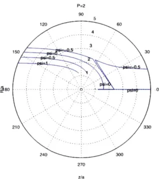
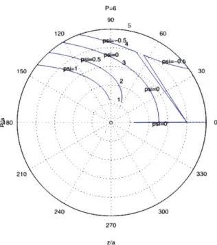
A simple model was developed for the charging of a spherical body using a corona discharge; it
ignores viscous effects and space charge due to the ions themselves. This model uses stream func-tion potential theory. The ion stream funcfunc-tion due to the electric field is:
Q = paV(1 - cos(9)) (3.15)
The ion stream function due to the wind is:
a3
- r2(1 - ) sin2
(0) (3.16)
The combined normalized stream function is:
= (1 - cos(O)) - P 2(1 - )sin2() (3.17)
2P p d
be-tween the tips and the sphere, r is the radius from the center of the sphere, p = r/a is the
nor-malized radius, and finally 9 is the angle of a given point from the incoming free stream flow (00).
Finally, the potential parameter is defined as, which compares the electric drift to wind contribu-tions:
P Aw
aw (3.18)
The streamline that follows the wind axis has a stream function 0 = 0, but this stream line
bi-furcates at the downstream point where the net ion velocity is zero because the wind drag just cancels the sphere's attraction. Setting b = 0 and cancelling the factor (1 - cos(O)) yields the
equation for the separatrix: the surface that separates trajectories that go to infinity from those that end on the sphere:
(p2 _ -)(1 + cos()) = 2P
p (3.19)
The ion stagnation point occurs at 0 = 0 on this surface. This gives us the equation for the
mini-mum radius beyond which an ion needs to be in order to be carried away by the wind.
2 1
p -- =P
P0 (3.20)
Distance to stagnation point vs. PotentiaLAWNd parameter P
-- - --- --- --- - - --- --- ... --... --- ---- _- -- --- --- --- ---- ---- --. .----. ...----. ..----.- -.-- -.-- ---.---- --2.8 2.6 2.4 22 2 1.8 1.6 1.4 1.2 0 1 2 3 4 5 6 7 8 9 P
Figure 3.2: Distance to Stagnation Point
![Figure 1.1: Aircraft being struck by Lightning [6]](https://thumb-eu.123doks.com/thumbv2/123doknet/13913740.449143/13.917.192.654.132.687/figure-aircraft-being-struck-by-lightning.webp)
![Figure 1.2: Negative Cloud to Ground Lightning Discharge [4]](https://thumb-eu.123doks.com/thumbv2/123doknet/13913740.449143/15.917.215.636.312.837/figure-negative-cloud-ground-lightning-discharge.webp)
![Figure 2.1: Determining Electrospray Starting Voltage [11]](https://thumb-eu.123doks.com/thumbv2/123doknet/13913740.449143/24.917.206.670.451.665/figure-determining-electrospray-starting-voltage.webp)
![Figure 3.1: 1 atm - Atmospheric Pressure [1]](https://thumb-eu.123doks.com/thumbv2/123doknet/13913740.449143/40.917.215.677.146.535/figure-atm-atmospheric-pressure.webp)