Alternative mortgage instruments : their distributional effects on homeownership, housing consumption, and the use of mortgage credit.

HOUSING CONSUMPTION, AND THE USE OF MORTGAGE CREDIT

by

Kerry Dean Vandell B.A., Rice University

1970

M.M.E., Rice University 1970

M.C.P.,, Harvard University 1973

Submitted in Partial Fulfillment of the Requirements for the

Degree of Doctor of Philosophy at the Massachusetts Institute of Technology July, 1977

SEP

6 1977

Certified by . . .. .. .. . . ... . . . . - .. Thesis Supervisor

12

Accepted by

ALTERNATIVE MORTGAGE INSTRUMENTS: THEIR DISTRIBUTIONAL EFFECTS ON HOMEOWNERSHIP,

HOUSING CONSUMPTION, AND THE USE OF MORTGAGE CREDIT

Kerry Dean Vandell

Submitted to the Department of Urban Studies and Planning on July 26, 1977 in partial fulfillment of the require-ments for the degree of Doctor of Philosophy.

This thesis examines the proposition that different mortgage instruments currently being suggested as

alterna-tives to the current instrument of housing finance (the FRM), can have very different consequences for different classes of households, affecting their likelihood of be-coming homeowners, their consumption of housing, and their use of mortgage credit. These consequences arise from

certain mortgage-related characteristics affecting the cash-flow cost of mortgage credit. In particular, it is sug-gested that certain types of variable-rate mortgages (VRM's) may have quite adverse effects on lower-income or

non-upwardly mobile households, whereas such instruments as the graduated-payment mortgage (GPM) and the price-level-adjusted mortgage (PLAM) would perform better than the current instrument for all households.

Chapter I develops this proposition. The current policy arguments against the introduction of the VRM are examined, and the extent to which these policy arguments have already been evaluated empirically is investigated. Little previous empirical work is found. Several alter-native mortgage instruments suggested as replacements or

supplements to the FRM are introduced and compared accord-ing to their present value and cash flow characteristics.

Chapter II develops from economic theory a struc-tural model of the demand for homeownership, housing con-sumption, and mortgage credit. In an imperfect financial market, it is found thatnot merely the present value costs,

the VRM, either as a replacement or a supplement to the FRM. It is found that the effect of VRM introduction on

different classes of households is dependent on supply and demand elasticities associated with certain mortgage-related characteristics. Finally, it is shown that in a competitive mortgage market situation with a number of instruments being offered as alternatives to the FRM,

greater efficiency will result, butnot all households will necessarily have greater access to lower cost credit than prior to alternative instrument introduction.

Chapter III develops the homeownership model.

Ordinary-least-squares regression analysis is carried out on cross-sectional data derived from the 1970 Survey of Consumer Finances. Two mortgage-related characteristics--the initial payment level and characteristics--the uncertainty in characteristics--the ex-pected payment burden trend--are found to be negatively related to the probability of homeownership. Alternative instrument simulation using the model suggests that the GPM and the PLAM would encourage slightly higher rates of homeownership among all household classes than cur-rently exist under the FRM. On the other hand, the VRM, especially a VRM indexed to a short-term interest rate series, is predicted to reduce homeownership rates.

Chapter IV develops the model of housing consump-tion by homeowners. The initial payment level is found

to be the only mortgage-related variable tested which affects housing consumption levels. Again, simulation results suggest that the GPM and the PLAM would be

superior to the FRM in encouraging housing consumption and the VRM would be inferior. Furthermore, the VRM is predicted to have an adverse impact upon lower-income,

young, elderly, and poor households.

Chapter V develops the models of mortgage credit usage and down payment levels. The initial payment level and the expected trend in mortgage payment burden are suggested to be influences upon mortgage credit usage,

whereas only the expected payment burden trend is suggested as an influence upon the down payment level. The

com-parative size of the mortgage-related coefficients in

these models identifies the degree of household sensitivity to mortgage characteristic changes and provides evidence about household response to them in its home purchase and

the highest per-household mortgage consumption levels with little redistributive impact. However, the FRM

is predicted to require the lowest down payment. The VRM, again, does not perform well, and is predicted

to result in little use of mortgage credit and high down payments.

Chapter VI summarizes the estimation and

simu-lation results of the previous three chapters. Each instru-ment (including the FRM) is ranked according to its

pre-dicted impact on homeownership levels, housing consumption, mortgage credit usage, and debt-equity ratios. Predicted distributional impacts are also tabulated. Certain types of instruments, especially the GPM and the PLAM, are

found to perform better than the FRM in several categories with little redistributional effects. The VRM, on the other hand, is found to perform significantly worse and to adversely affect lower income, young, elderly, and black households. The chapter concludes with a series of policy recommendations based upon results of the preceding

analysis.

Thesis Supervisor: Arthur P. Solomon

Title: Associate Professor of Urban Studies and Planning

My years spent at M.I.T. and the Joint Center for Urban Studies have been without doubt the most en-riching and satisfying of my life. They were also enjoy-able, thanks in large part to my wife, Debbie, who provided support, encouragement, and.a sympathetic ear during those years in Cambridge while we struggled through our respec-tive doctoral programs. She deserves the first and

greatest thanks.

To Art Solomon, my dissertation advisor and mentor since my admission to M.I.T., goes my deepest gratitude for his advice, recommendations, and help in negotiating the path through graduate school and through this thesis. Acting as his teaching assistant and working with him on

consulting activities provided me with strengthened under-standing of housing policy and applied research. His con-stant insistence on quality work and rigor in analysis considerably improved my research skills. His comments on earlier drafts of this thesis were invaluable.

To my dissertation committee also must go a

special thanks. My discussions with Don Lessard and his enlightened comments on my earlier drafts greatly enhanced my understanding of issues associated with residential

ideas. KentColton provided considerable insight into the institutional realities of the mortgage market.

Several faculty members not on my committee also aided in the conceptualization and evaluation of this dissertation. Most particularly, I wish to thank Mike O'Hare and Stan Fischer. Ben Harrison of M.I.T. deserves

special credit for his continuous encouragement of my research efforts through graduate school.

I also appreciate the association I have had with my colleagues at M.I.T. and the Joint Center. Howard Bloom,

Eric Brown, Ken Rosen, Margie Dewar, Lynn Sagalyn, and Penny Schaefer all provided help in a variety of areas associated with this work.

The National Science Foundation, the Bemis Fund, and the Joint Center for Urban Studies helped finance my graduate education. Additional funding for computations

was provided by the Department of Urban Studies and Planning. Vicki Davidson is gratefully recognized for her excellent typing of the final draft.

FLi.naLly, I wish to express my gratitude to bo th± my parents and my parents-in-law for -their support and

encouragement during my years of graduate school.

ACKNOWLEDGEMENTS . . . . . ... . . . . . . . . . . v

TABLE OF CONTENTS . . . . . . . . . . . . . . . . vii

INDEX OF FIGURES . . . . . . . . . . . . . . . . . xii

INDEX OF TABLES. . . . . . . . . . . . . . . . . . xv

Chapter I. INTRODUCTION . . . . . . . . . . . . . . 1

The Importance of Distributional Considerations in Alternative Mort-gage Introduction. . . . . . . . . . 1

The Inadequacies of Past Research. 3 The Present Study. . . . . . . . . . . 6

Alternative Instruments Considered . . . . 10

Conclusion . . . . . .... a. . . . . 16

Footnotes--Chapter I .. .. . ... . . 18

II. MODEL DERIVATION AND USE IN EXPLAINING THE EFFECTS OF ALTERNATIVE MORTGAGE INTRODUCTION . 9. .. .. .. ... .. 22

Theoretical Development . . . .. . . . 22

The Household's Opportunity Set. . . 22

The Cost of Mortgage Credit. . . .. 25

Present Value Component ... 26

Cash Flow Component . . . . . . . 29

Weighting of Present Value Versus Cash Flow Costs . . . . .... 30

Mr tgage Cost Response to Supply and Demand Changes.. . . . .. 32

Supply Changes. . . . . . . . 32

Demand Changes. . . . . . . . .33

The Cost of Equity Financing . . .

34-Present Value Component ... 34

Cash Flow Component . . . . . . . 35

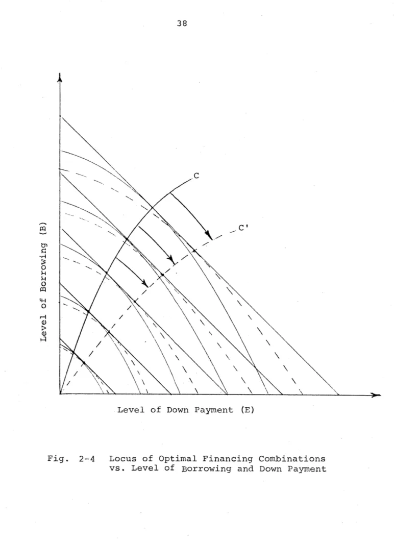
The Optimum Debt-Equity Locus. . 36' The Optimum Level of Housing . . . . Consumption . . .. . . . . . . . . 36

Using the Theoretical Framework to

Examine Market Reaction to the VRM. . . 43

VRM vs. FRM: Advantages and Dis-advantages from Point of View of Eorrowers . . . . . . . . . . . . 44

VRM vs. FRM: Advantages and Dis-advantages from Point of View of Lenders . . . ... 46

Applying the Theoretical Framework: Two Scenarios. . . . . . . . . . . . 49

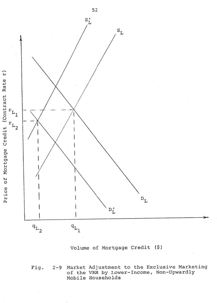
Exclusive Marketing of the VRM . . . 49

Supply Adjustments . . . . . . . . 50

Demand Adjustments . . . . . . . . 55

Equilibrium Adjustments. . . . . . 59

Competitive Marketing of Both the VRM and FRM. . . . . . . . . . 60

Conclusion . . . . . . . . . . . . . . . 65

Footnotes--Chapter II . . . . . . . . . . 67

III. AN EMPIRICAL INVESTIGATION OF THE EFFECT OF ALTERNATIVE MORTGAGE INSTRUMENTS UPON HOMEOWNERSHIP OPPORTUNITIES . . . . . . . . 75 Introduction. . . . 75 The Model . . . 81 Issues .. . . ... . . . ... . 81 Specification of Variables ... 84 Initial Specification. . . . . . . . 85 Variable Descriptions . . . . . . . 88 Final Specification. . . . . . . . .101 Estimation Procedures . . . . . . . . .103 Estimation Results . . . . . . . . . . .106

Income and Asset Influences on Tenure Choice. . . . . . . . . . . .108

Socioeconomic and Housing Market Influences on Tenure Choice. . . . .111

Mortgage-Related Influences on Tenure Choice . . . . . . . . . . .112

Simulation Results: The Introduction of Alternative Mortgage Instruments . .117 Caveats . . . . . . .. . .... ... 118

A Note on the Implications of Mixing Mortgage Instruments. . . . .123

Structural Demand vs. Equilibrium Analysis . . . . . . . . . . . . . .124

Aggregate Effects . . . . . . . . . . .126

Distributional Effects by Income. . . .130

Distributional Effects by Age . . . . .133

Distributional Effects by Race. . . . .137

Summary of Findings and Policy Implications. . . . . . . . . . . .. 139

Footnotes--Chapter III. . . . . . . . ..142 viii

OF ALTERNATIVE MORTGAGE INSTRUMENTS UPON HOUSING CONSUMPTION. . . . . . . . . . .

Introduction'... ... Short-Run Models . . . . . . . . Long-Run Equilibrium Models

The Model . . . . . . . . . . . . Issues . . . . . . . . . . . . . Model Theory . . . . . . . . . . Model Specification . . . . . . Estimation Procedures Estimation Results. ... Income and Asset Influences. . . Socioeconomic and Housing Market

Influences. .... .. .. .. Mortgage-Related Influences. . . . 153 .. . 155 . . . 159 . . . 162 . . . 162 . . . 163 . . . 165 . . . 169 . . . 170 . . . 171 . . . 174 . . . 175

Simulation Results: The Introduction of Alternative Mortgage Instruments. Aggregate Results. . . . . . . . . . Distributional Results by Income

Distributional Results by Age. . . . Distributional Results by Race

Summary of Findings and Policy

Implications . . . . . . . . . . . . Footnotes--Chapter IV . . . . . . . . V. AN EMPIRICAL INVESTIGATION OF THE EFFECTS

OF ALTERNATIVE MORTGAGE INSTRUMENTS UPON THE FINANCING OF RESIDENCES. . . . . . . Introduction . . . . . . . . . . . .. The Model . . . . . . . . . . . . . .

Issues . . . . . . . *... . ... . .. Model Theory and Specification . . .

Estimation Procedures. . . . . . . . Estimation Results . . . . . . . . . -.

Income and Asset Influences. . . . . Socioeconomic and Housing Market

Influences . . ... . .. .. .. Mortgage-Related Influences. . . . . Simulation Results: The Introduction

of Alternative Mortgage Instruments. Aggregate Effects. . . . . . . . . . Mortgage Credit . . . . . . . . . Down Payment Levels . . . . . . . Distributional Effects by Income .

Mortgage Credit . . . . . . . . . Down Payment Levels . . . . . . . Distributional Effects by Age

of Head ix 176 179 183 186 188 190 192 193 193 198 198 199 203 203 206 208 209 211 216 218 219 222 222 225 228 153

Mortgage Credit. . . . . . . . . . 228 Down Payment Levels. .. . . .... 230 Distributional Effects by Race. . . . 234 Mortgage Credit. . ... 234 Down Payment Levels. ... 234 Summary of Findings and Policy

Impli-cations . . . . . . . 238 Footnotes--Chapter V. . . . . . . . . . 242 VI. CONCLUSIONS AND POLICY IMPLICATIONS . . . 245 Empirical Results . . . . 245 Homeownership . . . . 249 Purchasing and Financing

Adjustments. . . . . . . . . . . . 250 Simulation Results .. .. . . .. . . 253 Policy Recommendations. . . . . . . . . 262 Footnotes--Chapter VI ..... . . . . . . 264 APPENDIX I

Continuous Time Stochastic Processes. . . . . 266 APPENDIX II

Derivation of Mortgage-Related Parameter Expressions for Alternative Mortgage

Instruments . . . . 278 APPENDIX III

Mathematical Derivation of the Models for Homeownership, Housing Consumption, and Mortgage Versus Down Payment

Financing . . . . . . . . . . . . . .. . . 293 APPENDIX IV

Variable Derivation from Computer Data-Tape . 304 APPENDIX V

Auxiliary Regressions: Determinants of

Mortgage-Related Variables. . . . . . . . . . 320 APPENDIX VI

Tables: Aggregate and Distributional Mortgage-Related Variable Values and

Simulation Results . . .. .. .... . 325

BIBLIOGRAPHY. . . . . . . .. . . . . . . . . . . . . 334 BIOGRAPHICAL NOTE . . .. . . .. . . . . . . . . . . 343

Page 2-1 Household Opportunity Set for Home

Financing ... . ... 24

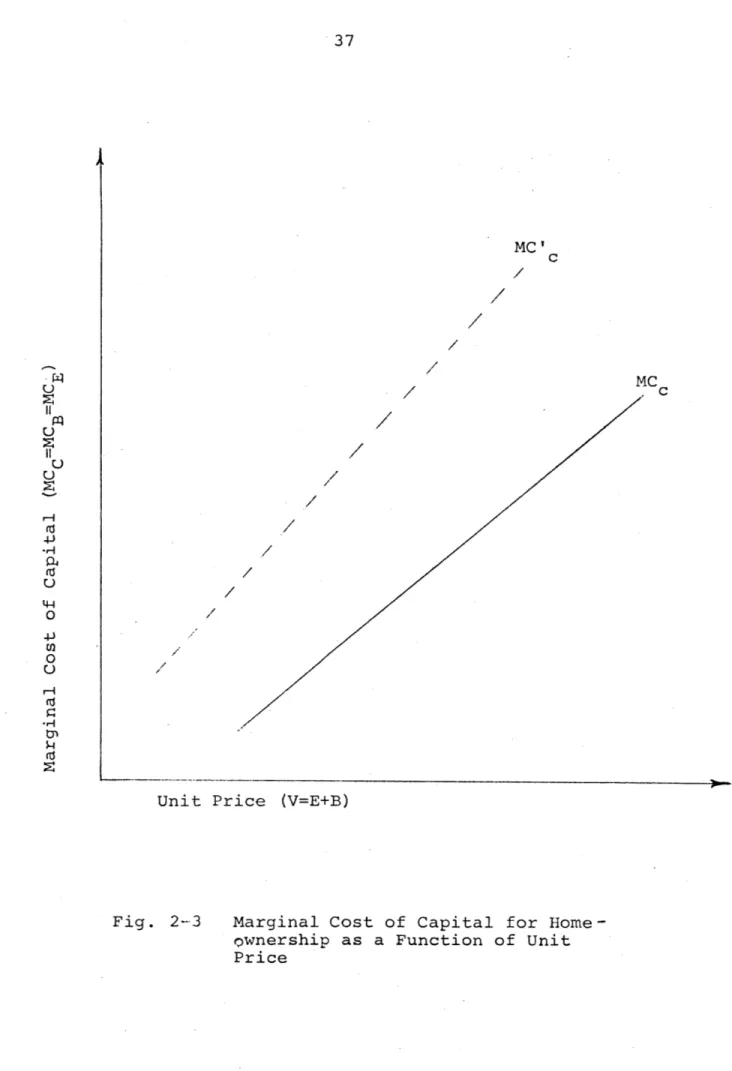
2-2 Marginal Cost of Mortgage and Down Payment Financing of Homeownership as a Function

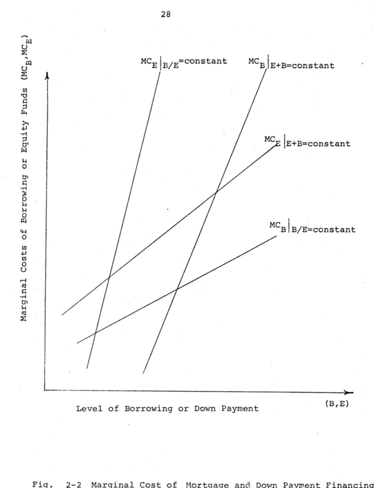
of the Level of Financing . . . . . . . . . 28 2-3 Marginal Cost of Capital for Homeownership

as a Function of Unit Price . . . . . . . . 37 2-4 Locus of Optimal Financing Combinations vs.

Level of Borrowing and Down Payment . . . . 38

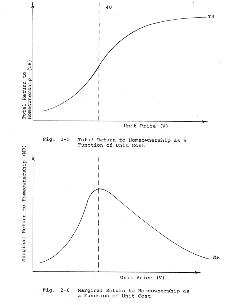
2-5 Total Return to Homeownership-as a Function

of Unit Cost . . . . . . . . . . . . . . . 40 2-6 Marginal Return to Homeownership as a

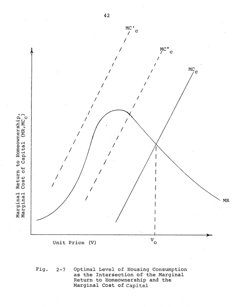
Function of Unit Cost . . . . . . . . . . . 40 2-7 Optimal Level of Housing Consumption as the

Intersection of the Marginal Return to Homeownership and the Marginal Cost of

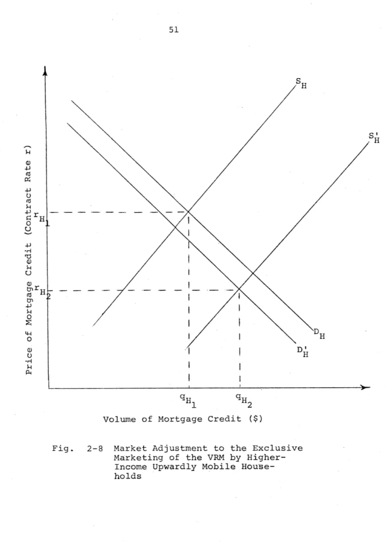
Capital . . . . . . . . . . . . . . . ... 42 2-8 Market Adjustment to the Exclusive Marketing

of the VRM by Higher-Income Upwardly

Mobile Households . . .. . . . . . . . . . .51 2-9 Market Adjustment to the Exclusive Marketing

of the VRM by Lower-Income, Non-Upwardly 52 Mobile Households . . . . . . . . . . . . .

2-10 Market Adjustment--FRM, Higher-Income Upwardly Mobile Households: The Case of Concurrent

Marketing with the VRM . . . . . . . . . . 62 2-11 Market Adjustment--FRM, Lower-Income,

Non-Upwardly Mobile Households: The Case

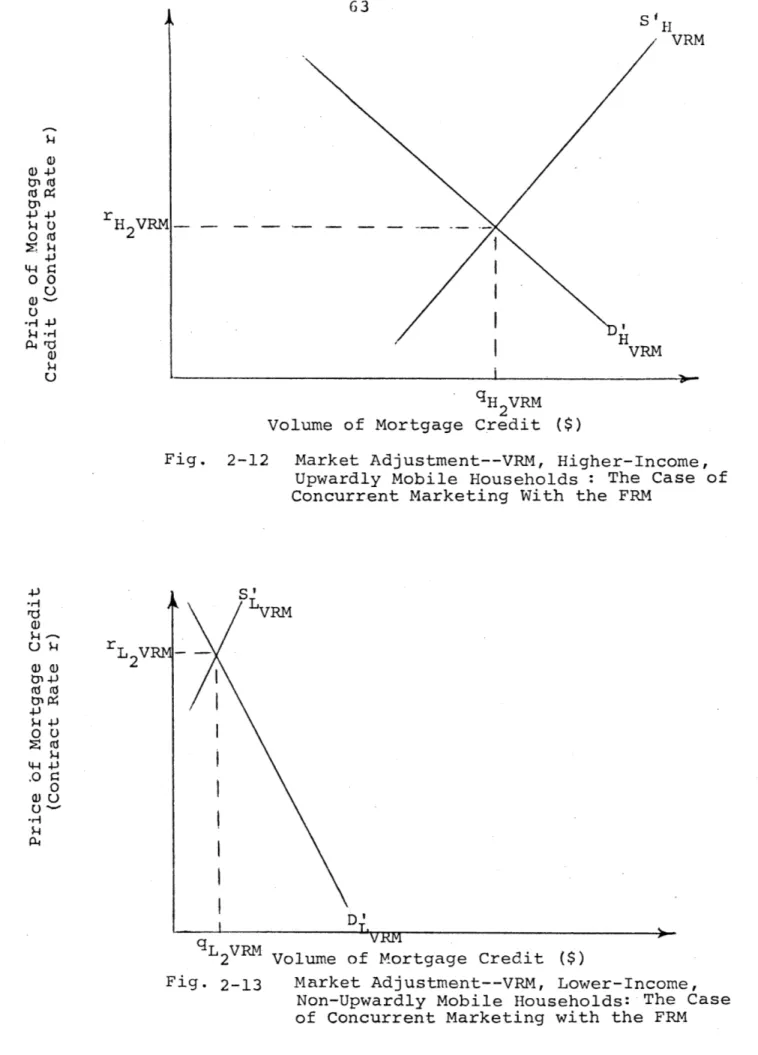
of Concurrent Marketing with the VRM . . 62 2-12 Market Adjustment--VRM, Higher-Income, Upwardly

Mobile Households: The Case of Concurrent

Marketing with the FRM . . . . . . . . . . 63 xii

Page 2-13 Market Adjustment--VRM, Lower-Income,

Non-Upwardly Mobile Households: The Case

of Concurrent Marketing with the FRM . . . 63 3-1 Predicted Change in Homeownership Rates (from

FRM Rates) by Instrument as a Function

of Family Income . . . . . . . . . . . . . 131 3-2 Predicted Change in Homeownership Rates (from

FRM Rates) by Instrument as a Function

of Age of Household Head . . . . . . . . . 134 3-3 Predicted Change in Homeownership Rates (from

FRM Rates) by Instrument as a Function

of Race . . . . . . . . . . . . . . . . . 138 4-1 Predicted Change in Housing Consumption

Levels Among Homeowners (from FRM Levels)

by Instrument as a Function of Family 184 Income . . . . . . . . . . . . . . . . . -.

4-2 Predicted Change in Housing Consumption Levels Among Homeowners (from FRM Levels) by

Instrument as a Function of Age of

Household Head . . . . . . . . . . . . . .187 4-3 Predicted Change in Housing Consumption Levels

Among Homeowners (from FRM Levels) by 189 Instrument as a Function of Race . . . . .

5-1 Predicted Change in Per-Household Mortgage Credit Usage (from FRM Levels) by

Instrument as a Function of Family 223 Income . . . . . . . . . .. . . .. . . .

5-2 Predicted Change in Down Payment Levels (from

FRM Levels) by Instrument as a Function of 226 Family Income . . . . . .

5-3 Predicted Change in Per-Household Mortgage Credit Usage (from FRM Levels) by

Instru-ment as a Function of Age of Family 229 Head . . . . . . . . . . . . . .

Page 5-4 Predicted Change in Down Payment Levels

(from FRM Levels) by Instrument as

a Function of Age of Family Head. . . . . 232 5-5 Predicted Change in Per Household Mortgage

Credit.Usage (from FRM Levels) by

Instrument as a Function of Race. . . . . 235

5-6 Predicted Change in Down Payment Levels (from FRM Levels) by Instrument as a

Function of Race . . . . 236 Al-l Price (p) as a Continuous Time Stochastic

Process . . . . 269

Page 3-1 Summary of Previous Econometric

Homeownership Studies . . . . . . . . . . . 78 3-2 Aggregate Simulation Results: Predicted

Equilibrium Rate of Homeownership

(OWN) by Mortgage Instrument . . . . . . . 127

4-1 Comparative Model Structures: The

Demand for Housing . . . . 157 4-2 Aggregate Simulation Results: Predicted

Housing Consumption Levels, by

Instrument . . . . . . . . . . . . . . . .180 5-1 Comparative Model Structures: The

Demand for Mortgage Credit . . . . . . .. 195

5-2 Mean Values for Initial Payment Level (P) and Expected Trend in Payment Burden (Tr) and Predicted Mortgage Credit Usage

(MORT), Down Payment Level (DOWN), and Debt-Equity Ratio by Mortgage

Instru-ment. . . . . . . . . . . . . . . . . . . . 5-3 Equilibrium Debt-Equity Ratios by

Instru-ment for Selected Household Groups . . . . . 224 6-1 Estimated Coefficients, Beta Values, and

Elasticities of Mortgage-Related Variables for Homeownership, Housing

Consumption, Mortgage Financing, and

Down Payment Equations. . . . .. . . -. . 248 6-2 Mortgage Instrument Performance Ranking

by Instrument and Merit Class . . . . . . . 254 Al-l Assumed Stochastic Processes for Component

Variables . . . . 270

A6-1 Mean Values of Initial Payment Level by

Income, Age, and Race for All Instruments . 326 xv

Page A6-2 Expected Change in Future Payment

Burden by Income, Age, and Race

for All Instruments . . . . 327

A6-3 Uncertainty in Future Payment Burden by Income, Age, and Race for All

Instruments . . . . 328 A6-4 Simulation Results--Predicted

Home-ownership Levels by Income, Age, and

Race for All Instruments. . . . . . . . . 329 A6-5 Simulation Results--Predicted Per-Household

Housing Consumption by Homeowners by Income, Age, and Race for All

Instru-ments . .. * . .. .. . .. .. . . - - - 330 A6-6 Simulation Results--Predicted

Per-House-hold Mortgage Credit Usage by Home-owners by Income, Age, and Race for

All Instruments . . . . 331 A6-7 Simulation Results--Predicted Per-Household

Down Payments by Homeowners by Income,

Age, and Race for All Instruments . . . 332 A6-8 Simulation Results--Predicted Debt-Equity

Ratios by Income, Age, and Race for All

Instruments . . . . -. 33

INTRODUCTION

The Importance of Distributional Considerations in Alternative

Mortgage Introduction

On three separate occasions since 1969, the Federal Home Loan Bank Board (FHLBB) has asked Congress to allow

it to permit federally chartered savings and loan asso-ciations to offer variable-rate mortgages (VRM's) as an alternative to the standard fixed-nominal-interest rate level-payment instrument (the FRM).1 These efforts have

been spurred by thrift institutions seeking to remedy periods of disintermediation, initiated by tight money conditions and exacerbated by the inflexible yield of the FRM. On all three occasions the FHLBB proposals have been rejected by Congress, largely due to the potential of adverse distri-butional consequences to certain groups of households

seek-ing to obtain credit for homeownership.2

Opponents of the introduction of the VRM and other alternative mortgage instruments postulate that these dis-tributional consequences would occur both on the supply and the demand sides of the mortgage credit market. On the

a change in default risk as perceived by lenders among certain borrower groups. This would be caused by expec-tations of changes in the level and uncertainty of future payment burdens and rates of equity accumulation under

these instruments. For those instruments and borrowers among whom default risk expectations would increase, len-ders would revise their underwriting practices--requiring higher down payments, lower maximum monthly payments or loan amounts as a fraction of income, or stricter credit standards. This would have the effect of rationing many households, now barely capable of sustaining homeownership under the FRM, out of the mortgage market.3

The major demand-side arguments against the intro-duction of alternative mortgage instruments are that many of these instruments alter the mortgage payment stream and

rate of amortization and shift some or all of the risk asso-ciated with future-interest rate changes from the lender to the borrower. The increased risk must be borne by the borrower in the form of increased uncertainty in future

4

payment levels, and rates of amortization. Many potential borrowers would find these new conditions difficult to

budget around and would naturally respond by lowering their demand for housing, mortgage credit, and homeownership.

The Inadequacies of Past Research

We have established that distributional arguments, whether they are valid or not, are acting as major

road-blocks to alternative mortgage instrument introduction. What evidence exists to provide a basis for these argu-ments? Plausible theoretical hypotheses, such as those in the previous subsection, have been formulated both to support and refute the possibility of adverse distributional conse-quences.5 However, theoretical analyses, although they are certainly important in presenting the logical possibilities, can only go so far. As one researcher has noted:

Clearly, most of these issues [associated with al-ternative mortgage instrument introduction] ulti-mately can only be resolved empirically, for there

is no other way to choose between the logical pos-sibilities presented.6

It is clear that the development of empirical models relating mortgage instrument characteristics to equilibrium

levels of homeownership, housing consumption, mortgage

credit usage, and down payment levels is necessary before any more definitive conclusions can be drawn about the pos-sible distributional effects of alternative mortgage in-strument introduction. However, because of data limitations and the lack of experience with alternative instruments in this country, such empirical work has not been forthcoming:

0_{No regression studies which have estimated the} deter-minants of homeownership have investigated the effect

fact that lenders' underwriting standards are widely recognized to be major constraints upon homeownership. Recently some computer simulation work has been

carried out which attempts to determine the relation-ship between mortgage characteristics and homeowner-ship. Most of these studies (e.g., Gelfand (1970)) are concerned with the FRM only; therefore, the form of the mortgage parameters (loan-to-value ratio, interest rate, amortization period) are useful only in evaluating changes in the terms of the FRM and not

in evaluating the impact of alternative instruments. The loan-to-value ratio, the contract interest rate,

and the amortization period could be identical for two types of mortgage instruments; yet the demand and

supply response to these instruments could differ radically, owing to differences in the expected trend and uncertainty in their payment streams and their rates of equity accumulation over time. One recent

study by Follain and Struyk (1977) simulates home-ownership increases under alternative instruments.

However, it only considers the lowered-initial pay-ment-level effect of such instruments and then only indirectly by assuming that the lowered payment is equivalent to an increase in income and then observing the income effect on homeownership.

*Regression studies which have related housing con-sumption to mortgage-related variables have been longitudinal aggregate studies which are incapable of investigating the microeconomic impact of

chang-ing debt payment streams under alternative instru-ments on individual households, whose income streams

are subject to variation and uncertainty. Moreover, as discussed above, the mortgage-related parameters used in these studies are capable of evaluating changes in the FRM only. These studies are also all "short-run" in that they are primarily interested in

explain-ing the role of mortgage terms in temporary credit rationing during tight money periods. All long-run equilibrium longitudinal studies except one have not included mortgage-related variables, according to the conventional wisdom that pure inflation-produced

changes in the terms of mortgage credit should have no long-run impact on housing consumption or mortgage credit usage.7 The sole exception is Kearl (1975) who includes a measure of the "tilt" in the real payment stream under inflation in a simulation of the macro-economic effects of alternative mortgage instrument

introduction.

*Regression studies which have related mortgage credit usage to mortgage-related variables have uniformly been longitudinal aggregate studies and, again

those mortgage-related variables which could be used

to evaluate the effects of alternative instrument

introduction. There are no empirical studies of the

effect of mortgage conditions on an individual

house-hold's down payment decisions.

The Present Study

The purpose of this dissertation is to address the

above expressed void in research efforts through an

em-pirical evaluation of the impact of alternative mortgage

instrument introduction upon the levels of homeownership,

housing consumption, and mortgage vs. down payment financing

by individual households. The primary hypothesis of the

study is that different instruments can have very different

consequences for different classes of households depending

upon the way in which mortgage characteristics interact

with individual household income and income expectations.

To test this hypothesis two major tasks will be undertaken:

1. Model Derivation and Estimation: A series of

models will first be derived theoretically and estimated

using multiple regression techniques. These will relate

the probability of homeownership and the levels of housing

consumption, mortgage credit usage,

and down payment

to income, assets, and other socioeconomic characteristics

of the household and to certain parameters associated with

mortgage credit. The objective of this estimation will be to show that in an imperfect credit market, mortgage parameters other than the contract rate can affect

homeownership, housing consumption, and mortgage credit usage.

The data set to be used for analysis is the 1970 Survey of Consumer Finances, which is disaggregated and cross-sectional, making possible the estimation of micro-economic impacts on individual households.8 This data set also allows computation of income and price expectations,

income and price uncertainty, household liquid assets, and housing finance parameters such as down payment, contract

interest rate, amortization period, and house value.

The mortgage-related characteristics to be included in the models are the initial annual payment per $100

borrowed, the expected trend in payment burden (payment-to-income ratio), and the uncertainty in the expected

trend in payment burden. The trend and uncertainty vari-ables have been defined as the trend and stochastic terms of a continuous time stochastic process for the payment burden.9

2. Model Simulation: The estimated models will then be used in a simulation exercise to predict the impact of a set of alternative mortgage instruments upon

home-ownership, housing consumption, and mortgage vs. down payment financing. This task will be carried out by calculating

ment and substituting these values into our estimated models. 10

Three important points should be emphasized at this time which affect the strength and interpretation of our simulation results. The first is that our empirical estimations will represent structural demand relationships only and not general or even partial equilibrium results. A general equilibrium analysis would require a macro-economic model of the U.S. economy, and would be an

ex-tremely complex undertaking. A partial equilibrium model would require separate supply relationships. Such

re-lationships cannot be adequately constructed in our model due to limitations on data availability. Thus the con-tract rate, period of amortization, and other mortgage-related parameter values are not determined endogenously. This means that upon alternative instrument introduction, we must make certain judicious assumptions about these parameter values after the economy adjusts to the new

instruments. The strength of the simulation results- is reduced accordingly.

The second point which affects the strength of our simulation results is that because of data limitations they are incapable of completely taking into account both cash flow and present value influences on borrower demand.

credit and would be the only mortgage-related influences which matter in a perfect financial market. Cash flow in-fluences reflect the disutility associated with the mort-gage payment stream as it relates to the borrowing house-hold's income stream. Such influences can be highly im-portant in imperfect financial markets and are the justi-fication behind those arguments concerning differential reaction to alternative instrument introduction. Thus our simulation results will be somewhat biased as a result except under certain restrictive assumptions. This issue will be discussed in depth in Chapters II and III.

The third point affecting interpretation of our simulation results relates to the likelihood that any alternative mortgage introduction would be a supplement rather than a replacement for the FRM. When considering the effects of alternative instruments upon homeownership, housing consumption and mortgage credit usage, the really relevant question is the impact of a mix of mortgage

instruments, rather than a single instrument. To properly attempt to answer such a question, general equilibrium information must be available about the relative interest rate and maturities at which such a mix of instruments

would be offered after the economy adjusts to the introduc-tion. Such an analysis is extremely complex and beyond the

scope of this research. We show later that our analysis makes possible a crude estimation of the most desirable type

tions about contract rates and maturities are made. How-ever, our basic analysis remains the evaluation of the impact of a single instrument if it alone were offered. Thus, if we wish to interpret our results in terms of a mix of instruments, rather than concluding a certain

instrument would have a very adverse impact on a certain class of households, we should conclude that that instru-ment would very likely not be chosen by such households.

Alternative Instruments Considered

The set of alternative instruments to be simulated included (1) the standard variable-rate mortgage (VRM),

(2) the graduated payment mortgage (GPM), (3) the price level adjusted mortgage (PLAM), and (4) the income-linked mortgage (ILM). The first three instruments--especially

the VRM--have been most.often suggested as supplements or replacements for the FRM. The ILM has been little

dis-cussed and will very likely never be introduced. However, it presents an interesting case in our simulations and has been included on that basis. Following is a brief

definition and discussion of each instrument according to differences in debt payment streams and expected impacts on borrowers and lenders.

(1) The standard VRM has a fixed contract ma-turity, as does the FRM, but the payment level fluctuates

according to changes in the mortgage interest rate over time, which is tied to an "index" short-term rate (VRMS) or long-term rate (VRML). This variation in the payment stream is the characteristic of this instrument sought after by lenders, since payment levels would tend to in-crease during high interest-rate, tight-money periods when disintermediation ordinarily becomes a problem under the FRM. Increased payment levels imply less of a squeeze

on the lender's cash flow, hence making possible more mort-gage loans. In addition, they make possible a higher in-terest paid on savings, thus further reducing disinter-mediation.

The VRM is potentially undesirable to certain borrower groups for the same reason it is desirable to lenders. The uncertainty in future payment levels under the VRM makes budgeting by borrower households more diffi-cult, especially if their income fluctuations are great or are highly uncorrelated with the payment fluctuations. This increased uncertainty could also affect lending be-havior insofar as it adversely affects default risk by

certain groups.

The initial payment level of the standard VRM would very likely be somewhat lower than that for the FRM at equilibrium, since the instrument would theoretically have to be offered at a "discount" to entice borrowers

where-the VRM has been offered by some state-chartered thrift institutions for years, this discount in the con-stant rate was originally one-fourth to one-half percent-age -point, although more recently, VRM's are being offered at the same rate as the FRM.

(2) The GPM would, like the FRM, be a fixed nominal-interest-rate, fixed-maturity instrument. However, it

differs from the FRM in that it specifies an a priori gradu-ated, rather than level, nominal payment stream. The

graduation rate can theoretically be adjusted for individual household needs: the lender could lower the initial pay-ments, to help low-current-income households such as young

professionals, or lower later payments to help high-current-income, but low-expected-income households, such as those about to retire. These adjustments, of course, would change the expected trend in future payment burdens in a direction which would tend to offset the effects of the adjusted initial payment level. However, if the gradua-tion rate is properly chosen, the net advantage can be maximized for each household. Regardless of the

gradua-tion rate chosen, the uncertainty associated with future payment burdens under the GPM is identical to that under

the FRM, since the payment stream is fixed a priori. Tak-ing all those considerations together, we conclude the GPM is superior to the FRM from the standpoint of the borrower and would be expected to have a positive demand effect.

The Department of Housing and Urban Development has re-cently allowed introduction of the GPM on a trial basis.

From the standpoint of the lender, the GPM would have no advantage over the FRM, and could even prove

slightly inferior. Payment levels under the GPM, like those under the FRM, would not adjust according to unfore-seen monetary or inflationary conditions. In fact, if the lender's mortgage portfolio were somewhat -undiversi-fied with respect to mortgage origination period and rate of graduation, cash flows to the lending institution could become quite volatile under the GPM. A lender would pre-sumably be even less willing to give a positively-graduated GPM during--or just prior--to an expanded tight money

period than he would an FRM, since his immediate cash flow benefits would be lower. These points suggest the

pos-sibility that there might be negative cyclical supply ef-fects associated with the GPM.

A second way in which the GPM could prove inferior to the FRM from the lenders' standpoint is its effect on default risk. Lower initial payments under the GPM imply not only a lower initial payment burden, which tends to reduce default risk, but also a lower rate of equity ac-cumulation, which tends to increase default risk. The net effect of these two influences is uncertain a priori.

(3) The PLAM is characterized by initially lower nominal monthly payments which float upward according to

offered at the "real" interest rate. For a required nomi-nal yield of eight percent under expected six-percent

inflation, it could be offered at somewhere around two percent. As under the FRM and the standard VRM, the maturity is held constant.

The PLAM would be more desirable than the VRM to borrowers for three reasons. First, the initial pay-ment levels would be lower than those under the VRM.

Se-cond, the expected payment stream would very likely not fluctuate as much, since prices are generally less vola-tile than interest rates. Finally, the PLAMI could offer a relatively fixed payment burden over the life of the mortgage if nominal income rises at the rate of inflation. However, the PLAM would also prove undesirable to borrowers in one respect. It would not offer the inflationary hedge of the FRM and would not be desirable to less-upwardly-mobile households or those on fixed income because payments would increase with prices rather than remaining fixed as under the FRM.

The PLAM would be of some advantage to lenders since it would compensate for inflation-produced increases in nominal rates. In addition, to the extent that periods of inflation are correlated with tight-money periods, it would also provide some increase in cash flows during tight-money periods, thus counteracting disintermediation

and the "lending-squeeze." Individual households,

how-ever, could experience adverse lender reaction to the

PLAM in those cases in which default risk is increased

by the increased trend and uncertainty in expected

pay-ment burden, offsetting decreased risks due to the lower

initial payment.

(4) The ILM is a nominal-interest-rate mortgage

with payments indexed to each individual's income stream.

Thus the maturity of the instrument necessarily floats

to allow for differences in income streams over time. A

household with increasing income over time would pay off

a given mortgage much sooner than one with decreasing

income.

The flexible maturity of this instrument does

not strictly allow the ILM to be simulated in the

framework we will establish. Our framework was not

successful in evaluating the effects of maturity

ad-justments.

This restriction is acceptable as long

as maturities are invariant, as they are for the VRM,

the GPM, and the PLAM; and as long as the maturity effect

is primarily a cash flow effect. For an instrument in

which these conditions are not true, it is necessary, in

order for our analytic framework to be valid, to assume

maturities only vary slightly or households discount highly

future mortgage payments and care little about equity

the investment--objective of homeownership. To analyze

the ILM we have therefore necessarily made this

assump-tion, keeping in mind, however, the above caveats.

The

ILM

would be very desirab.e to the borrower,

since it totally transfers risk of future payment burden

increases to the lender.

If a single fraction of income

were set as the index for all borrowers, it would be

pro-portionately more beneficial to lower-income households,

since they currently, on the average, spend a higher

pro-portion of their income on housing under the FRM than do

higher-income households.

The lender, however, would be less satisfied with

the ILM, since he must bear full risk associated with

individual income fluctuations. Thus there could be adverse

supply consequences for certain groups of borrowers if

the ILM were introduced as the sole replacement for the

FRM (a possibility which is highly unlikely).

These supply

consequences, however, may be mitigated by the fact that:

(1) cash flows overall could tend to increase during periods

of credit stringency to the extent that nominal incomes

were correlated with interest rates, and (2) controlling

the payment burden could serve to reduce default risk.

Conclusion

It is hoped that this analysis will contribute

toward a resolution of the debate over consumer

acceptability of alternative mortgage instruments. Empiri-cal estimation of the sensitivity of homeownership levels, housing consumption, and mortgage vs. down payment financing the type and terms of the credit instrument could render

valuable assistance in formulating public policies aimed both at fostering a healthy thrift industry and at equit-able treatment of all classes of households.

The remainder of this dissertation shall be organ-ized as follows. Chapter II shall theoretically derive the models to be estimated empirically and shall use these models to formally outline the major contentions set forth

by opponents of alternative mortgage introduction.. The third through fifth chapters shall present the estimation and simulation results for the models of homeownership,

housing consumption, and mortgage-vs.-down payment-financing respectively. In the final chapter, conclusions will be drawn about the overall desirability of certain alternative instruments for meeting consumer needs, and policy implica-tions of the research will be noted.

In 1969; on August 10, 1972; and on August 1, 1974.

2_{In 1969 the FHLBB withdrew the proposal to} authorize federally chartered savings and loan associa-tions to introduce VRM's after extended correspondence with Congressional Banking Committee members. The 1972 pro-posal, backed by recommendations of a 1969 study of the

savings and loan industry (the Friend Report) and the 1971 Report of the President's Commission on Financial

Struc-ture and Regulation (the Hunt Commission Report), again was rebuffed by Congress. The 1974 proposal was turned down after extensive hearings in both houses of Congress, at which numerous representatives of consumer groups testified

against the measure. Congressman Ferdinand St. Germain (D., R.I.), Chairman of the House Banking Subcommittee on Financial Institutions Supervision, Regulation, and Insur-ance, which considered the proposal, condemned it as "a cruel hoax on the consumer."

3_{See, for example, the testimony of Steven M.} Rohde, in U. S. Congress, House of Representatives, Com-mittee on Banking, Currency and Housing, "Variable Rate

Mortgage Proposal and Regulation Q," Hearings before the 18

Subcommittee on Financial Institutions Supervision, Regulation, and Insurance, 94th Congress, 1st Session, April 8, 9, and 10, 1975, pp. 374-376.

4_{Ibid., pp. 376-377.}

5_{For a theoretical argument in favor of} alter-native instruments, see Cohn and Fischer (1974), pp. 54-57, and U. S. League of Savings Associations (1974).

6_{Prell (1971), p. 19; see also Kearl (1975),}

p. 15.

7_{For a discussion of short-run versus long-run} studies of housing and mortgage credit demand, see Kearl, Rosen, Swan (1974).

8_{Described in Katona, et al., (1971).}

9_{See Appendix I for a brief introduction to the} use of continuous time stochastic processes in

mort-gage research.

1 0_{See Appendix II for a formal derivation of these}

parameter values for each instrument.

11Under _{the Housing and Community Development Act}

of 1974, HUD can undertake an experimental financing program by insuring innovative mortgage instruments with

amortization plans which correspond to anticipated varia-tions in family income (Section 245 of the National Housing Act). In August, 1976, the Senate Subcommittee on Housing and Urban Affairs of the Senate Banking Committee held

hearings on the need to use this power to restructure the traditional mortgage instrument to meet current needs. HUD testified at those hearings on their public solicitation of alternative mortgage proposals and their serious con-sideration of the experimental introduction of some form of the GPM.

1 2_{In the extreme, a household with a low enough} expected income stream paying a small enough fraction of its income as mortgage payment would never pay off the

principal on its mortgage and, in fact, could build up ever-increasing interest charges. The permitted income frac-tion and the expected income stream of each borrower,

therefore, impose an effective limit on the permitted lend-ing ceillend-ing which would allow the mortgage to be fully amor-tized in a reasonable period of time (30-40 years).

1 3_{Consider the following example, which} illus-trates the possibility of erroneous conclusions by making this assumption in extreme situations: a household paying

a certain percentage of its income for mortgage payments under an ILM would find all loan amounts equally desirable' under our model, in spite of the fact that above a certain

loan ceiling the household will never amortize the mort-gage and at loan amounts above this ceiling will continue

to build up an ever-increasing balance due to unpaid accumulated interest.

MODEL DERIVATION AND USE IN EXPLAINING THE EFFECTS OF ALTERNATIVE MORTGAGE

INTRODUCTION

This section (1) will develop using economic theory the models of homeownership, housing consumption, and mortgage and down payment financing to be estimated and (2) will use this theoretical framework to summarize the arguments of proponents and opponents of alternative instruments about reaction to these instruments by dif-ferent household types.

Theoretical Development1

The Household's Opportunity Set

Consider a household which is evaluating the home-purchase decision. It must answer three interrelated

questions: (1) whether it wants to rent or own, (2) the expenditure it wishes to make on a home, and (3) the ex-tent to which it wishes to invest its own equity in the house or finance through borrowing.

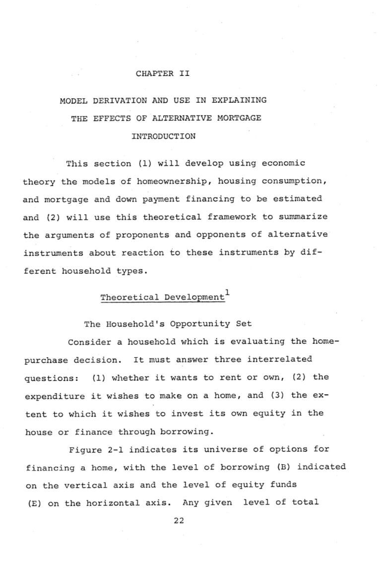
Figure 2-1 indicates its universe of options for financing a home, with the level of borrowing (B) indicated on the vertical axis and the level of equity funds

(E) on the horizontal axis. Any given level of total 22

housing expenditures V₀ = (E + B

)

since the levels of borrowing and down payment are perfect substitutes for financing a given volume of housing.

The household's opportunity set is limited by several constraints. First, the level of its liquid assets A prevents a down payment beyond that level.

Second, its income, Y₀ , is an absolute limit on the monthly mortgage payments it can make and hence the level of

bor-rowing it can incur (B (Y0 )). The asset constraint is more likely to be effective than the income constraint,

since a household generally spends 25 percent or less of its income on mortgage payments but often spends virtually all of its liquid assets on a down payment.2

A second set of institutionally imposed supply constraints may also effectively limit the opportunity set of the household. On the equity side, the lending institution, to lower its risk exposure, may require the down payment to be a certain fraction of the total unit price (E₀ = tVW₀ ). This fraction for conventional loans is generally in the 10- to 25-percent range. This con-straint is shown as the radial labeled Dmin in Figure 2-1

1-

F

On the borrowing side, again to reduce its risk exposure, the lending institution may set a maximum ceil-ing on the level of monthly mortgage payment burden the

E A min B(Y

)

V/

2

/

/7max

Level of Down Payment (E)

Fig. 2-1 Household Opportunity Set for Home Financing

household may incur, usually as a certain fraction a of monthly income. The general rule-of-thumb for this

con-straint is usually one week's pay or 25 percent. This con-straint is shown as the horizontal line labeled B (a Y ) in Figure 2-1.

Finally, on both the borrowing and equity side, the lending institution may seek to limit its risk exposure by setting a maximum ceiling on the size home the house-hold may purchase, usually as a certain multiple y of annual income. y is generally considered to be in the

2.0 to 2.5 range. This constraint is shown as the isoquant

VMax Y in Figure 2-1.

Note that all constraints can vary for different individuals and over time, depending on lenders' rules-of-thumb, borrowers' income and wealth positions, and mortgage terms. The constrained opportunity set for the

household is shown as the shaded area in Figure 2-1. We shall next consider the costs of equity and borrowed funds.

The Cost of Mortgage Credit

When we use the term mortgage cost in this sertation, we are describing a household's perceived dis-utility associated with present and future mortgage pay-ments. This disutility arises from two sources which we

The present value or yield component is the dis-utility associated with the present value of future expected mortgage payments (net after income tax reductions) dis-counted at a discount rate which is characteristic of each household along with any uncertainty in that present value.

It is this component which is the only component relevant in a perfect financial market. In fact, in a perfect fi-nancial market, if the household discount rate is equal to the market rate, the cost of mortgage credit is equal to the amount borrowed, and the cost of homeownership collapses to the price of the house (down payment + mortgage princi-pal = price of house). The present value component totally

ignores the pattern of future mortgage payments (except for tax treatment effects) as they relate to the household's in-come stream. If this component were the only component being considered as the "cost" of mortgage credit, then such in-struments as the FRM, ILM and GPM offered at the same con-tract rate would only differ according to the time pre-ference of individual households and according to the

slightly different income-tax reduction patterns under each instrument. The VRM and PLAM would differ from the FRM also according to their respective risks associated with their present values, since the future cash flow streams are unknown a priori. The present value component may be represented by the following variables: normalized initial payment level, expected trend in payments, uncertainty in

in that duration, and finally permanent income, assets, and demographic characteristics which proxy for the house-hold's discount rate and the shape of its present-value utility function.

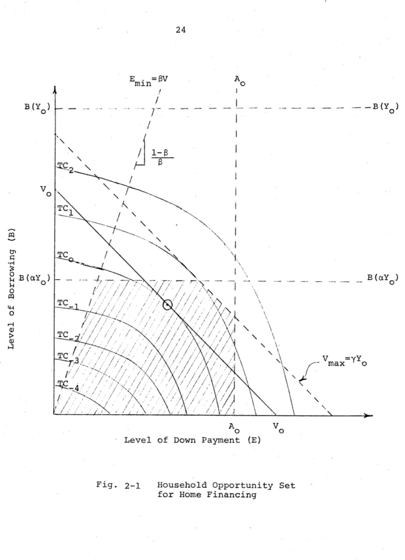
It would be expected that the marginal present value cost of mortgage credit would rise with the levelof borrow-ing, both for a constant debt-equity ratio and for a constant total purchase price. _{(MCB B/E=Constant and MCB B+E=Constant}

in Figure 2-2.) This would be because of supply considera-tions. In the first case, lenders would perceive higher risk of default from a household which commits itself to a larger mortgage, hence a larger payment burden, and would respond by increasing the contract rate on mortgage credit available to the household. In the second case, not only is the household committing itself to higher payment bur-dens, the debt-equity ratio is increasing with an increase in borrowing. This would imply the household would have a lower equity stake in the household thus increasing the risk of default, and the lender would be exposed to a higher risk of loss in case of default. The lender would

there-fore respond by increasing his contract (gross) interest rate to yield him an expected net yield to offset the risk.

The terms of mortgage credit would not only be functions of the level of borrowing. Lenders would also be expected to adjust their contract rates and allowed maturities according to current and permanent income, assets, and demographic characteristics of the household,

MCE IB/E=constant E+B=constant 1 >J1 -H 0 44 0 4 0 LH -(B,E) Level of Borrowing or Down Payment

Fig. 2-2 Marginal Cost of Mortgage and Down Payment Financing of Homeownership as a Function of the.

Level of Financing

IC

:;EE+B=constant

MCB

IB/E=constant

and characteristics of the mortgage payment stream which might affect the risk of default. In the case of the mortgage payment stream, the cash flow characteristics

of each instrument type and the rate of equity accumulation become relevant. A final factor which affects lender be-havior with respect to setting contract rates and

matu-rities is the yield in the market. To be offered on the market, the mortgage must be competitive in terms of net yield relative to its risk for instruments of comparable liquidity.

Cash Flow Component

The cash flow component of mortgage cost is the present value of the disutility associated with expected mortgage payments as they relate to future borrower income,

discounted at each household's discount rate, along with any uncertainty in that present value. This component is relevant in an imperfect financial market where bor-rowers cannot readily and costlessly convert income to assets, assets to income, current income to future income, or future income to current income. It may represent

insolvency due to cash flow mismatch, a forced adjustment of other desired expenditures to offset adverse payment/ income outcomes, or simply the inconvenience and discom-fort of having to engage in further financing in order to match income and housing expenditures.