HAL Id: hal-02267655
https://hal.archives-ouvertes.fr/hal-02267655
Submitted on 19 Aug 2019
HAL is a multi-disciplinary open access
archive for the deposit and dissemination of
sci-entific research documents, whether they are
pub-lished or not. The documents may come from
teaching and research institutions in France or
abroad, or from public or private research centers.
L’archive ouverte pluridisciplinaire HAL, est
destinée au dépôt et à la diffusion de documents
scientifiques de niveau recherche, publiés ou non,
émanant des établissements d’enseignement et de
recherche français ou étrangers, des laboratoires
publics ou privés.
An automatic parametric approach for WCET analysis
of C programs
D Kebbal
To cite this version:
D Kebbal. An automatic parametric approach for WCET analysis of C programs. ERTS2 2010,
Embedded Real Time Software & Systems, May 2010, Toulouse, France. �hal-02267655�
An automatic parametric approach
for WCET analysis of C programs
D. Kebbal
Institut de Recherche en Informatique de Toulouse
118 route de Narbonne - F-31062 Toulouse Cedex 9 France
[email protected]
Abstract: In this paper, we propose a static worst-case execution time (WCET) analysis approach aimed to automatically extract flow information related to pro-gram semantics. This information is used to reduce the overestimation of the calculated WCET. We focus on flow information related to loop bounds and infea-sible paths. The approach handles loops with multi-ple exit conditions and non-rectangular loops in which the number of iterations of an inner loop depends on the current iteration of an outer loop. The WCET of loops is analytically computed and expressed as sum-mations function of the loop bounds. This avoids un-folding loops while providing tight and safe WCET es-timate. Furthermore, the provided WCET expressions are expressed symbolically function of the program input parameters. This allows to reduce the WCET computing cost while providing tight WCET values. In-deed the WCET of each piece of code is expressed as symbolic expression which is instantiated each time that piece is called in the program. The flow analy-sis uses an enhanced symbolic execution approach based on symbolic execution and an analytic method in order to avoid unfolding loops performed by sym-bolic execution-based approaches.
Keywords: automatic parametric flow analysis, block-based symbolic execution, symbolic expression simplification.
1 Introduction
Real-time systems validation requires the knowledge of the execution time or bounds on the execution time of programs. WCET analysis is a well used approach in the validation of the temporal constraints of hard real-time systems.
WCET analysis consists of computing an upper bound on the execution time of a program rather than the ex-act WCET values as this problem is undecidable in the general case. However, it is imperative that WCET analysis must guarantee the Safeness and the Tight-ness of the provided WCET values in order to keep real-time systems predictable and their cost financially reasonable.
Static WCET analysis performs a high-level static analysis of the program source or object code. This avoids working on the program input data. For each component of the program, an upper bound of the ex-ecution time is estimated. Static WCET analysis tech-niques proceed generally in three phases [3, 6]: flow analysis, low-level analysis and WCET estimate com-puting. Flow analysis characterizes the execution se-quences of the program’s components, their execu-tion frequency, etc. (execuexecu-tion paths). In this phase, the execution costs of basic blocks are assumed to be constant. Generally, two types of flow informa-tion may be extracted. The first category is related to the program structure and may be extracted automat-ically. The second category is related to the program functionality and semantics. This includes informa-tion about loop bounds and feasible/infeasible paths especially. Low-level analysis computes an execution time estimate of each program component on the tar-get hardware architecture. Finally in the calculation phase, a WCET estimate of the whole program can be computed based on the results of the two previous steps.
The remainder of the paper is organized as follows: in the next section we review the related work. Sec-tion 3 describes and discusses the flow-analysis ap-proach. In section 4, we address the algebraic evalu-ation of iterative scopes issue. Section 5 presents and discusses a formalism used to handle the generated symbolic expressions and their simplification. Finally, in section 6, we conclude the paper and present some perspective issues.
2 Related work
One of the most popular methods for static WCET analysis are based on path analysis, which proceed by explicitly enumerating the set of the program exe-cution paths [9, 1]. [8] describes a method based on cycle-level symbolic execution to predict the WCET of real-time programs on high performance processors. The main drawbacks of those approaches lie in the im-portant number of the generated paths which scales exponentially with the program size. Another class
of approaches called IPET1 do not explicitly
enumer-ate all program paths. In this class of techniques, the problem of the WCET estimation is converted to an ILP2problem [6, 10, 3].
However, all those approaches involve the program-mer in the flow information determination process, es-pecially the flow information related to program se-mantics (feasible/infeasible paths, loop bounds, etc.). Though the provided flow information may be highly precise, this is an error-prone problem. Interval-based abstract interpretation and symbolic execution meth-ods [4, 2] allow to automatically extract flow infor-mation related to program semantics. These meth-ods proceed by rolling out the program (especially loops) until it terminates, which is very costly in time and memory. In [5], an approach for determining loop bounds analytically without unfolding them is pre-sented. They consider loops with multiple exit condi-tions and non-rectangular loops, in which the number of iterations of an inner loop depends on the current iteration of an outer loop. However, they provide only numerical WCET values which may lead to overesti-mation in the case of multiple calls to the same sub-program. [7] presents a parametric approach based on abstract interpretation and a method for counting integer points in polyhedra. The approach seems complex in practice. [1] proposes a method to com-pute symbolic WCET. However, they use an annota-tion mechanism involving the programmer in the flow analysis process.
We propose an automatic flow analysis approach which allows to automatically compute WCET of each piece of code (function, loop, etc.) as symbolic ex-pression. This allows to obtain tighter but safe WCET values as the computed symbolic expression can be instantiated for each specific call to the subprogram and nested loops leading to tighter WCET values with a low cost. We use an enhanced symbolic execu-tion method which avoids unfolding complex blocks by evaluating each complex block analytically.
3 Flow analysis approach
In this section, we describe our approach aimed to au-tomatically extract the flow information related to pro-gram functionality (bounds on loop iterations, infeasi-ble paths, etc.). We use a data flow analysis approach based on symbolic execution in order to derive values of variables at different points in the program.
3.1 Program representation
We use the control flow graph (CFG) formalism to ex-press the control flow of the program to be analyzed. The source code of the program is decomposed into
1Implicit Path Enumeration Techniques. 2Integer Linear Programming.
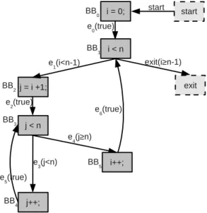
a set of basic blocks. Two fictitious blocks, label-ed startand exit are added. We assume that all execu-tions of the CFG start at the start block and end at the exitblock. Figure 2 illustrates an example of a control flow graph of a program where the C source code is shown in figure 1.
Formally, the program is represented by the graph G = (B, E), where B, the set of the graph nodes, represents the program basic blocks and the set of edges (E) the precedence constraints between the basic blocks.
void sort(unsigned int n) { unsigned int i, j;
for (i=0; i<n-1; i++) { for (j=i+1; j<n; j++) { }
} }
Figure 1: Example of a C program
Figure 2: CFG of the C example
3.2 Scopes and scope graphs
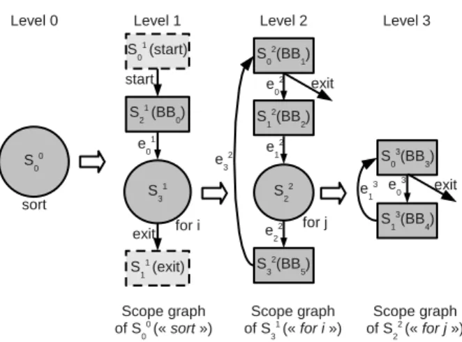
In addition, we use the notion of scope where a set of scopes of level l are grouped into a scope of level l− 1. Scopes correspond to complex pro-gramming language features (loops, conditional state-ments, functions, modules, etc.). The scope compo-sition starts at the lowest level and may be recursively carried out until the CFG level. Figure 3 illustrates the
Figure 3: The scope graphs of the example
scope graphs constructed for the C example of the fig-ure 1. A scope S is composed of a set of sub-scopes related by edges, a set of header blocks and one or more exit edges. Each scope S of level l is defined by a scope graph describing its structure (figure 3). Formally, a scope S of level l is defined by the formula 1 and composed of: a number of sub-scopes (Ss); a
set of header blocks (Sh
s ⊆ S); a set Esof edges
con-necting the sub-scopes; and one or more exit edges (Ee
s⊆ Es).
S = {Ss, Ssh, Es, Ees}. (1)
The S’s sub-scopes set Ssis composed of scopes of
higher levels (m > l). The set of edges Es is
con-structed as follows: each edge of the CFG connect-ing two nodes belongconnect-ing to two different sub-scopes si and sj of Ss forms an edge of level l from si to
sj. Edges to scopes outside Ssproduce edges of exit
type. Redundant edges are eliminated. In figure 3, in the graph of scope S31corresponding to the for i loop, the edge e2connecting the basic blocks BB2and BB3
in the CFG yields the edge e21.
A header block is a basic block executed when the execution flow reaches the scope for the first time. In-formally, header blocks correspond to loop and selec-tion condiselec-tion test blocks. The set of headers of the scope S is denoted by Sh
s. The set of header-blocks
of the scope S1
3 is {BB1} (figures 2 and 3). Notice that
a well-structured code yields scopes with one header block. When the execution of the scope is terminated, the control flow leaves the scope through an exit-edge. The set of outgoing edges from a scope S is denoted by Ee
s. The set of exit-edges of the scope S31 is {exit}
(figure 3). When the execution of a scope must be re-peated, this is done by transferring the execution flow to the header block through a back-edge. The set of back-edges of a scope S is denoted by Eb
s. The set of
back-edges of the scope S31is {e23} (figure 3).
3.3 Path condition and path action
Each elementary edge e in the CFG is associated a path condition P C(e) which is a Boolean predicate conditioning the execution of that edge with respect to the program state s at the source node of the edge. Likewise, each basic block bb applies a block action BA(bb) which represents the effect of the execution of the sequence of all statements of the block on the pro-gram state s (symbolic execution rules). The path ac-tion of a path p denoted P A(p) is the sequence of the block action of all blocks constituting that path. Like-wise the path condition of a path is the “logical and” of the path condition of all edges forming that path. In order to compute the path action of a path p, we consider the set of program variables assigned in dif-ferent blocks of the path Vp. Let BA(bb, v) be the
func-tion applied by the basic block bb on the variable v ∈ Vp which represents the effect of the execution of all
statements of the block on v. The action applied on v by p (P A(p, v)) is the sequence of block action applied by all blocks forming p in the order they appear in p. P A(p, v) = (BA(bb0, v); BA(bb1, v); . . . ; BA(bbn−1, v))
may be represented by an expression of the form av+b such that a and b are integer constants (a > 0). This hypothesis implies that the loop induction variable (ex. i) update statement is of the form i= a ∗ i + b.
4 Algebraic evaluation of iterative scopes As we have seen, a key idea of our approach is the way the iterative scopes are handled. Indeed, itera-tive scopes are not folded, rather than they are ana-lytically evaluated. To do, the number of iterations of such iterative scope must be algebraically computed and the WCET of that scope is estimated based on the computed number of iterations. Furthermore, the values of assigned variables inside the scope must be computed. In the following, we address those issues in more details.
4.1 Analytic evaluation of the number of iterations of loops
In order to analytically compute an estimate of the number of iterations of a loop path, we define the suite (in) as follows:
(
i0= N1∈ N
in+1= ain+ b ∀n ∈ N
(2)
This suite can be redefined as follows: (
i0= N1
in+1= in+ an(b + N1(a − 1)) ∀n ∈ N
(3)
The general term of this suite can be infered using the following relation:
in= i0+ n−1 X k=0 [ik+1− ik] = N1+ n−1 X k=0 [ik+ ak(b + N1(a − 1)) − ik] = N1+ n−1 X k=0 [ak(b + N 1(a − 1))] = ( N1+ (b + N1(a − 1))a n−1 a−1 when a >1 N1+ nb when a= 1 (4) The number of iterations I is defined by the relation iI−1≤ N2(the loop limit). That is:
(
N1+ (b + N1(a − 1))a
I−1−1
a−1 ≤ N2when a >1
N1+ (I − 1)b ≤ N2when a= 1
By knowing that the number of iterations I is a posi-tive integer, we can deduce its value as the greatest integer less than or equal to the right-hand side of the inequality, which yields:
I= ( ⌊loga(1 + (N2−N1)(a−1) b+(a−1)N1 )⌋ + 1 when a > 1 ⌊N2−N1 b ⌋ + 1 when a= 1 (5)
For each elementary path condition expression e of the form i op expr, the following parameters are eval-uated:
• Interval type: the interval is qualified as raised if opis “≤”, constant if op is “=” and undervalued if opis “≥”. Expressions containing “<” and “>” op-erators are converted to expressions containing “≤” and “≥” operators exclusively.
• Direction: if the variable i in increased in the path action (P A(p)), the direction is positive and neg-ative if i is decreased in P A(p). If i is never up-dated along with the path, the direction is con-stant. The direction is determined by the expres-sion a∗ i + b and is positive when the expression (a − 1)N1+ b is positive and negative when it is
negative and constant when it is 0.
The direction and the interval type are used to deter-mine if a loop is empty before applying the formula 5. Thus, in case when the interval is raising and the di-rection is positive the number of iterations is given by the formula 5 if N1 ≤ N2 and 0 otherwise. Likewise,
when the interval is undervalued the number of itera-tions is∞ when N1 ≥ N2 and 0 otherwise. For
ex-ample, in the”f or i” loop of the sort example (i = 0, i < n− 1, i = i + 1), a = 1, b = 1, N1 = 0. The
expression(a − 1)N1+ b is evaluated to 1. The
direc-tion is then positive and the interval type is underval-ued. Therefore the loop is not empty. The computed number of iterations and the WCET are expressed as
symbolic expressions using the guarded expressions mechanism presented in the next section. The pro-vided symbolic guarded expressions will be instanti-ated when numerical values are provided.
Complex path condition expressions are evaluated by decomposing them recursively into elementary Boolean expressions related by logical operators (e1 ∧ e2 or e1 ∨ e2). Each elementary conditional expres-sion e is of the form i op expr, where op is a re-lational operator and expr is an integer valued ex-pression. Each expression is then analytically eval-uated as described above. Then the number of iter-ations Ierelated to e and the resulting symbolic state
Se are calculated. The total number of iterations is
determined from the number of iterations of all sub-expressions of e as follows: Ie1∨e2 = max(Ie1, Ie2) and Ie1∧e2 = min(Ie1, Ie2).
4.2 Updating variables assigned inside iterative scopes
In this subsection, we address the algebraic evalua-tion of variables assigned inside the iterative scope body. For this purpose, we assume a general form on the assignment statements of variables inside iterative scopes that can be updated analytically.
s= c ∗ s + d ∗ i + e; i= a ∗ i + b; p= k;
q= f (v1, v2,· · · );
(6)
Such that: a, b, c, d, e, k are expressions which remain constant within the iterative scope body. a, b ∈ N. f is a function. v1, v2,· · · are variables which may be
assigned inside the loop scope and different from p. In order to analytically compute the values of the vari-ables at the end of iterative scope, we first consider the following suite:
( u0∈ R
un+1= gun+ rtn+ s ∀n ∈ N
(7)
be expressed by the following: un= gnu0+ r n−1 X k=0 gktn−k−1+ s n−1 X k=0 gk ∀n > 0 (8) = gnu 0+ rtn−1 1−( g t) n 1−g t + s gn−1 g−1 = gnu 0+ rt n−gn t−g + s gn−1 g−1 when p1 gnu 0+ rngn−1+ sg n−1 g−1 when p2 u0+ rt n−1 t−1 + sn when p3 u0+ rn + sn when p4 gnu 0+ sg n−1 g−1 when p5 s when p6 u0+ sn when p7 ∀n > 0 (9) with: p1= (t 6= 0 ∧ g 6= 1 ∧ g 6= t) p2= (g = t ∧ g 6= 0 ∧ g 6= 1) p3= (g = 1 ∧ t 6= 0 ∧ t 6= 1) p4= (g = t = 1) p5= (t = 0 ∧ g 6= 1 ∧ g 6= 0) p6= (g = t = 0) p7= (g = 1 ∧ t = 0)
The evaluation of the two variables s and i at the end of the iterative scope, may be done by means of the two suites(sn) and (in) defined as follows:
s0 ∈ R. i0 ∈ Z. sn+1= csn+ din+ e in+1= ain+ b (10)
Using the formulas 7 and 9 (g= a, r = 0, s = b), we can prove easily that the value of the variable i at the iteration n may be given by the following expression:
in= b when a= 0 i0+ nb when a= 1 ani 0+ ba n−1 a−1 when a >1 (11)
The value of the variable s can be infered as follows: sn+1= cn+1s0+ di0An+ Bn (12) Such as: A0= 1 An+1= cAn+ an+1= cAn+ aan And: B0= e Bn+1= cBn+ n X k=0 dakb+ e = cBn+ db n X k=0 ak+ e = cBn+ db an+1− 1 a− 1 + e
Again using the formulas 7 and 9 (g = c, r = t = a, s= 0), we can prove easily that the value of the vari-able A at the iteration n may be given by the following expressions: An= ( cn(n + 1) when c= a an+1−cn+1 a−c when c6= a
Finally still using the formulas 7 and 9 (g = c, r = dba a−1,
t= a, s = e − db
a−1), we can deduce the value of Bnas
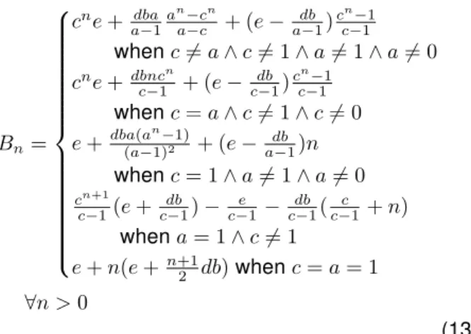
follows: Bn= cne+ dba a−1 an−cn a−c + (e − db a−1) cn−1 c−1 when c6= a ∧ c 6= 1 ∧ a 6= 1 ∧ a 6= 0 cne+dbncn c−1 + (e − db c−1) cn−1 c−1 when c= a ∧ c 6= 1 ∧ c 6= 0 e+dba(a(a−1)n−1)2 + (e − db a−1)n when c= 1 ∧ a 6= 1 ∧ a 6= 0 cne+ (e + db)cn−1 c−1 when a= 0 ∧ c 6= 1 ∧ c 6= 0 e+ db when c = a = 0 e+ n(e + db) when c = 1 ∧ a = 0 ∀n > 0 In case of a= 1, we have: Bn+1= cBn+ db n X k=0 1k+ e = cB n+ (n + 1)db + e B0= e
Therefore, we can easily demonstrate3that:
Bn = e n X k=0 ck+ db n−1 X k=0 (n − k)ck = cn+1 c−1(e + db c−1) − e c−1 − db c−1( c c−1+ n) when a= 1 ∧ c 6= 1 e+ n(e +n+1 2 db) when c = a = 1 ∀n > 0
We then simplify the formula which gives: Bn= cne+ dba a−1 an−cn a−c + (e − db a−1) cn−1 c−1 when c6= a ∧ c 6= 1 ∧ a 6= 1 ∧ a 6= 0 cne+dbncn c−1 + (e − db c−1) cn−1 c−1 when c= a ∧ c 6= 1 ∧ c 6= 0 e+dba(a(a−1)n−1)2 + (e − db a−1)n when c= 1 ∧ a 6= 1 ∧ a 6= 0 cn+1 c−1(e + db c−1) − e c−1− db c−1( c c−1 + n) when a= 1 ∧ c 6= 1 e+ n(e +n+12 db) when c = a = 1 ∀n > 0 (13) To summarize, variables assigned within iterative scopes are evaluated in many manners following the way they are assigned inside the scope i.e. the as-signment statement type:
• Statements of type s in the formula 6. In this case, the variable is evaluated using the formula 12. • Statements of type i in the formula 6. In this case,
the variable is evaluated using the formula 11. • Statements of type q in the formula 6. In this case,
the variable value is given by replacing in the ex-pression of the function f the variables v1, v2,· · ·
by their final values.
• Statements of type p in the formula 6. The vari-able remains unchanged (p= k).
4.3 Scope-based symbolic execution
Symbolic execution consists of using symbols instead of numbers as input values for a program execution. The program (especially loops) is then rolled out until it terminates which represents a symbolic execution. The values of program variables are represented with symbolic expressions and the program output values are expressed as function of the program input sym-bols [2].
We use an enhanced symbolic execution approach which avoids rolling out loops reducing thus the com-plexity of the symbolic execution. In our approach, a symbolic execution state is represented by a triple < V, P C, SP >, where:
• V is the set of pairs < v, e >, which holds all com-binations of variables values that are possible at the control point. V = {< v1, e1 >, < v2, e2 >
, . . . , < vn, en >} denotes a symbolic state where
the variables v1, v2, . . . , vn have been assigned
the expressions e1, e2, . . . , en;
• P C is the path condition expressing the condi-tions under which that path is taken;
• SP is the instruction pointer referring to the next sub-scope in the scope graph to execute.
Initially, the input parameters and all the other vari-ables are initialized using symbols. SP points to the header block of the scope and P C is set to true. Sym-bolic execution of a program takes a symSym-bolic state and a rule which corresponds to the block action of the sub-scope referred to by SP and returns the symbolic states resulting from the execution of the rule. When SP points to the header block for the second time, the defined loop path is analytically evaluated follow-ing the process described in subsection 4.1, which re-duces the complexity of the approach. Furthermore, only a subset of the symbolic states set of the program are computed. For this purpose, we associate to each scope a set of control points which correspond to its terminal symbolic states set. A control point state is composed of the set of the scope variables with their initial values Vinas well as the corresponding terminal
state. The evaluation of a scope yields the set of its control points and a symbolic WCET expression as-sociated to each exit control point. Figure 4 shows the scope-based symbolic execution of the scope S2
2.
A WCET value based on the number of iterations is computed and associated to each symbolic state. The number of iterations, WCET expressions and the vari-able values are computed using the formulas 5, 11 and 12 discussed in the previous subsection.
? ? ? ? V={<j,α0>,<n,α1>} P C=true SP=S3 0, wcet=0 V={<j,α0>,<n,α1>} P C=α0≤α1−1 SP=S3 1, wcet=1 V={<j,α0>,<n,α1>} P C=α0≥α1 SP=S2 3, wcet=1 V={<j,α0>,<n,α1>} P C=α0≤α1−1 SP=S3 0, wcet=2 V={<j,α1>,<n,α1>, P C=α0≤α1−1 SP=S2 3, wcet=2(α1−α0)+1 s0 s1 s2 s3 s4
Figure 4: Evaluation of the scope S2 2
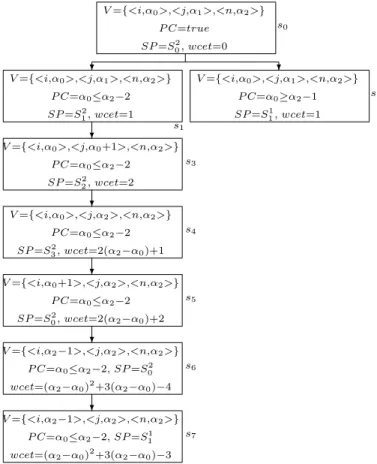
In order to understand how the non rectangular loops problem is handled by the block-based symbolic ex-ecution, we consider the evaluation of the scope S1 3
(the ”f or i” outer loop) shown on the figure 5. The application of the scope S2
2 on the state s3
gener-ates only one state (s4) because on the figure 4,
ap-plying the control point corresponding to the state s2
leads to a false path condition (a false path) since α0 ≤ α2− 2 ⇒ α0 ≥ α2− 1 leads to a f alse value.
The WCET expression in the state s7is computed as
wcet(s7) = α2−α0−2 X x=0 (2α2− 2α0− 2x + 2) = (α2− α0)2 + 3(α2− α0) − 4
The final WCET of the scope S00corresponding to the
”sort” function is given by n2 + 3n − 2 rather than
(n−1)(2n+1)+2) = 2n2−n−1 induced by the methods
that don’t handle rectangular loops, which reduces the estimated WCET value by a factor of 2.
? ? ? ? ? ? ? V={<i,α0>,<j,α1>,<n,α2>} P C=true SP=S2 0, wcet=0 V={<i,α0>,<j,α1>,<n,α2>} P C=α0≤α2−2 SP=S2 1, wcet=1 V={<i,α0>,<j,α1>,<n,α2>} P C=α0≥α2−1 SP=S1 1, wcet=1 V={<i,α0>,<j,α0+1>,<n,α2>} P C=α0≤α2−2 SP=S2 2, wcet=2 V={<i,α0>,<j,α2>,<n,α2>} P C=α0≤α2−2 SP=S2 3, wcet=2(α2−α0)+1 V={<i,α0+1>,<j,α2>,<n,α2>} P C=α0≤α2−2 SP=S2 0, wcet=2(α2−α0)+2 V={<i,α2−1>,<j,α2>,<n,α2>} P C=α0≤α2−2, SP =S02 wcet=(α2−α0)2+3(α2−α0)−4 V={<i,α2−1>,<j,α2>,<n,α2>} P C=α0≤α2−2, SP =S11 wcet=(α2−α0)2+3(α2−α0)−3 s0 s1 s2 s3 s4 s5 s6 s7
Figure 5: Evaluation of the scope S1 3
5 Handling symbolic expressions
The block-based symbolic execution proceeds by evaluating each scope independently and uses sym-bols as input values for all unknown variable values. Consider the evaluation of of the scope S2
2 presented
in the figure 4.
The direction value i.e. the expression(a − 1)N1+ b
in evaluating s3 is 1. If the direction is evaluated to
a symbolic expression, the number of iterations and WCET expressions will be conditioned by the effec-tive value of the direction parameter. For instance con-sider that the assignment statement of j is j= 2 ∗ j + 1 in the loop body, (a = 2, b = 1, N1 = α0). Then the
direction evaluates to α0 + 1. Therefore, the
num-ber of iterations I in s4 is given by: ⌊α1−α20−1⌋ + 1
when the direction is positive i.e. α0+ 1 > 0 since
N1 ≤ N2 = α0 ≤ α1− 1 is always true (implied by
the path condition of the state s3). Likewise when the
direction is negative i.e. α0+ 1 < 0, I evaluates to ∞
(since we always have N1≤ N2). And when the
direc-tion is constant i.e. α0+ 1 = 0 the number of iterations
is∞.
In order to express such conditional expressions when computing the number of iterations and variable val-ues expressions, we use the symbolic guarded ex-pression mechanism [1]. Hence, the number of iter-ations of the scope S2
2 can be expressed by the
fol-lowing guarded expression: [α0 > −1](⌊α1−α20−1⌋ +
1) + [α0≤ −1]∞
Guarded expressions constitute a powerful mecha-nism which is used to evaluate symbolically the WCET of a piece of code using conditional expressions. A guarded expression denoted [c]e is evaluated as fol-lows:
[c]e = (
e if c
0 otherwise (14) However, handling symbolic guarded expressions im-plies the use of simplification properties which may be different from the standard algebra. Hence, in addi-tion to standard properties (commutativity, associativ-ity, distributivassociativ-ity, . . . ), we adopt some other properties to simplify arithmetic guarded expressions.
ge op[f alse]e = ge with op ∈ {+, ×} ge+ [c]0 = ge
[c]e × [c]1 = [c]e ge× [c]0 = [true]0
− [c]e = [c](−e)
[c]e1+ [c]e2= [c](e1+ e2)
[c]e1× [c]e2= [c](e1× e2) [c]e2 X i=[c]e1 [c]e = [c] e2 X i=e1 e
These properties can be easily demonstrated. The last property is particularly used when evaluating an-alytically nested loops and generating new symbolic states as shown by the example presented at the end of the previous subsection.
6 Conclusion
Real-time systems must be predictable in time and memory in order avoid undesirable consequences when the temporal constraints are not respected es-pecially in critical environments. WCET analysis has
became an important research field in the area of em-bedded systems in which the emphasis is on reducing the gap between the theoretical worst case values and the observed ones.
WCET analysis may be done statically on the pro-gram source or object code which avoids dealing with the program input data and target hardware platforms, but results in overestimated values. Therefore, tech-niques allowing to tighten the WCET estimates are re-quired. However, these techniques are complex be-cause they deal with program semantics.
We proposed a practical symbolic approach aimed to automatically extract flow information related to pro-gram semantics which will be used to tighten the WCET estimates. The method presents a reduced complexity, at least on the theoretical level, in terms of time and memory by avoiding unfolding iterative scopes. Moreover, the approach provides tight WCET values since it provides WCET of the system compo-nents (functions, etc.) as symbolic expressions func-tion of the component input parameters, which allows to instantiate them with numerical values for each call of the component. Furthermore, the approach han-dles non rectangular loops and loops with multiple exit conditions and eliminates implicitly most of the in-feasible paths. Indeed, non rectangular nested loops and infeasible paths constitute an important source of overestimation in WCET analysis.
We are implementing and evaluating a prototype of the method. Furthermore, we plan to extend the ex-pression used to evaluate loops to Presburger formu-las and use the results obtained on those formuformu-las.
References
[1] G. Bernat and A. Burns. An approach to symbolic worst-case execution time analysis. In 25th IFAC Workshop on Real-Time Programming, Palma, Spain, May 2000.
[2] A. Coen-Porisini, G. Denaro, C. Ghezzi, and M. Pezzè. Using symbolic execution for verifying safety-critical systems. In 8th European software engineering con-ference, pages 142–151, New York, USA, 2001. ACM Press.
[3] A. Ermedahl. A modular Tool Architecture for Worst-Case Execution Time Analysis. PhD thesis, Uppsala University, 2003.
[4] J. Gustafsson and A. Ermedahl. Automatic deriva-tion of path and loop annotaderiva-tions in object-oriented real-time programs. Journal of Parallel and Distributed Computing Practices, 1(2):61–74, 1998.
[5] C. Healy, M. Sjodin, V. Rustagi, D. Whalley, , and R. van Engelen. Supporting timing analysis by auto-matic bounding of loop iterations. Journal of Real-Time Systems, 18(2-3):129–156, May 2000.
[6] Y.-T. S. Li and S. Malik. Performance analysis of em-bedded software using implicit path enumeration. In ACM SIGPLAN Workshop on Languages, Compilers and Tools for Real-time Systems, La Jolla, California, June 1995.
[7] B. Lisper. Fully automatic, parametric worst-case ex-ecution time analysis. In 3rd International Workshop on Worst-Case Execution Time Analysis, WCET 2003, pages 99–102, Polytechnic Institute of Porto, Portugal, 2003.
[8] T. Lundqvist and P. Stenström. An integrated path and timing analysis method based on cycle-level sym-bolic execution. Real-Time Systems, 17(2-3):183–207, 1999.
[9] C. Y. Park and A. C. Shaw. Experiments with a pro-gram timing tool based on source-level timing schema. Journal of Real-Time Systems, 1(2):160–176, Septem-ber 1989.
[10] P. Puschner and A. V. Schedl. Computing maximum task execution- a graph-based approach. Real-Time Systems, 13(1):67–91, July 1997.