Clouds in the atmosphere of the super-Earth exoplanet GJ�1214b
The MIT Faculty has made this article openly available. Please sharehow this access benefits you. Your story matters.
Citation Kreidberg, Laura, et al. “Clouds in the Atmosphere of the Super-Earth Exoplanet GJ 1214b.” Nature, vol. 505, no. 7481, Jan. 2014, pp. 69–72. © 2018 Springer Nature Limited
As Published http://dx.doi.org/10.1038/NATURE12888
Publisher Springer Nature
Version Final published version
Citable link http://hdl.handle.net/1721.1/118780
Terms of Use Article is made available in accordance with the publisher's policy and may be subject to US copyright law. Please refer to the publisher's site for terms of use.
arXiv:1401.0022v1 [astro-ph.EP] 30 Dec 2013
Clouds in the atmosphere of the super-Earth exoplanet
GJ 1214b
Laura Kreidberg1, Jacob L. Bean1, Jean-Michel D´esert2,3, Bj¨orn Benneke4, Drake Deming5, Kevin B. Stevenson1
, Sara Seager4
, Zachory Berta-Thompson6,7
, Andreas Seifahrt1
, & Derek Homeier8 1
Department of Astronomy and Astrophysics, University of Chicago, Chicago, IL 60637 2
CASA, Department of Astrophysical & Planetary Sciences, University of Colorado, Boulder, CO 80309
3
Department of Astronomy, California Institute of Technology, Pasadena, CA 91101 4
Department of Physics, Massachussetts Insitute of Technology, Cambridge, MA 02139 5
Department of Astronomy, University of Maryland, College Park, MD 20742 6
Department of Astronomy, Harvard University, Cambridge, MA 02138 7
MIT Kavli Institute for Astrophysics and Space Research, MIT, Cambridge, MA 02139 8
Centre de Recherche Astrophysique de Lyon, ENS Lyon, Lyon, France
Recent surveys have revealed that planets intermediate in size between Earth and Neptune
(“super-Earths”) are among the most common planets in the Galaxy1–3. Atmospheric
stud-ies are the next step toward developing a comprehensive understanding of this new class of
object4–6. Much effort has been focused on using transmission spectroscopy to
character-ize the atmosphere of the super-Earth archetype GJ 1214b7–17, but previous observations did not have sufficient precision to distinguish between two interpretations for the atmosphere. The planet’s atmosphere could be dominated by relatively heavy molecules, such as water (e.g., a 100% water vapor composition), or it could contain high-altitude clouds that obscure its lower layers. Here we report a measurement of the transmission spectrum of GJ 1214b at near-infrared wavelengths that definitively resolves this ambiguity. These data, obtained with the Hubble Space Telescope, are sufficiently precise to detect absorption features from a high mean molecular mass atmosphere. The observed spectrum, however, is featureless. We rule out cloud-free atmospheric models with water-, methane-, carbon monoxide-, nitrogen-,
or carbon dioxide-dominated compositions at greater than 5σ confidence. The planet’s
at-mosphere must contain clouds to be consistent with the data.
We observed 15 transits of the planet GJ 1214b with the Wide Field Camera 3 (WFC3) in-strument on the Hubble Space Telescope (HST) between UT 27 September 2012 and 22 August 2013. Each transit observation consisted of four orbits of the telescope, with 45-minute gaps in phase coverage between target visibility periods due to Earth occultation. We obtained time-series spectroscopy from 1.1 to 1.7µm during each observation. The data were taken in spatial scan
mode, which slews the telescope during the exposure and moves the spectrum perpendicular to the dispersion direction on the detector. This mode reduces the instrumental overhead time by a factor of five compared to staring mode observations. We achieved an integration efficiency of 60 – 70%. We extracted the spectra and divided each exposure into five-pixel-wide bins, obtaining spectro-photometric time series in 22 channels (resolutionR ≡ λ/∆λ ∼ 70). The typical signal-to-noise
per 88.4 s exposure per channel was 1,400. We also created a “white” light curve summed over the entire wavelength range. Our analysis incorporates data from 12 of the 15 transits observed, be-cause one observation was compromised due to a telescope guiding error and two showed evidence of a starspot crossing.
The raw transit light curves for GJ 1214b exhibit ramp-like systematics comparable to those seen in previous WFC3 data10, 18, 19. The ramp in the first orbit of each visit consistently has the
largest amplitude and a different shape from ramps in the subsequent orbits. Following standard procedure for HST transit light curves, we did not include data from the first orbit in our analysis, leaving 654 exposures. We corrected for systematics in the remaining three orbits using two tech-niques that have been successfully applied in prior analyses10, 18, 20. The first approach models the
systematics as an analytic function of time. The function includes an exponential ramp term fit to each orbit, a visit-long slope, and a normalization factor. The second approach assumes the mor-phology of the systematics is independent of wavelength, and models each channel with a scalar multiple of the time series of systematics from the white light curve fit. We obtained consistent re-sults from both methods (see Extended Data Table 1), and report here rere-sults from the second. See the Supplementary Information and Extended Data Figs. 1 – 6 for more detail on the observations, data reduction, and systematics correction.
We fit the light curves in each spectroscopic channel with a transit model21 to measure the
transit depth as a function of wavelength; this constitutes the transmission spectrum. See Figure 1 for the fitted transit light curves. We used the second systematics correction technique described above and fit a unique planet-to-star radius ratio Rp/Rs and normalization C to each channel and each visit, and a unique linear limb darkening parameter u to each channel. We assumed a
circular orbit22 and fixed the inclinationi = 89.1◦, the ratio of the semi-major axis to the stellar radiusa/Rs = 15.23, the orbital period P = 1.58040464894 days, and the time of central transit
Tc = 2454966.52488 BJDTDB. These are the best fit values to the white light curve.
The measured transit depths in each channel are consistent over all transit epochs (see Ex-tended Data Fig. 5), and we report the weighted average depth per channel. The resulting trans-mission spectrum is shown in Figure 2. Our results are not significantly affected by stellar activity, as we discuss further in the Supplemental Information. Careful treatment of the limb darkening is critical to the results, but our limb darkening measurements are not degenerate with the tran-sit depth (see Extended Data Fig. 4) and agree with the predictions from theoretical models (see Extended Data Fig. 6). Our conclusions are unchanged if we fix the limb darkening on theoret-ical values. We find that a linear limb darkening law is sufficient to model the data. For further description of the limb darkening treatment, see the Supplementary Information.
The transmission spectrum we report here has the precision necessary to detect the spectral features of a high mean molecular mass atmosphere for the first time. However, the observed spectrum is featureless. The data are best fit with a flat line, which has a reducedχ2
compare several models to the data that represent limiting case scenarios in the range of expected atmospheric compositions17, 23. Depending on the formation history and evolution of the planet, a high mean molecular mass atmosphere could be dominated by water (H2O), methane (CH4), car-bon monoxide (CO), carcar-bon dioxide (CO2), or nitrogen (N2). Water is expected to be the dominant absorber in the wavelength range of our observations, so a wide range of high mean molecular mass atmospheres with trace amounts of water can be approximated by a pure H2O model. The data show no evidence for water absorption. A cloud-free pure H2O composition is ruled out at
16.1σ confidence. In the case of a dry atmosphere, features from other absorbers such as CH4, CO,
or CO2 could be visible in the transmission spectrum. Cloud-free atmospheres composed of these absorbers are also excluded by the data, at 31.1, 7.5, and 5.5σ confidence, respectively. Nitrogen
has no spectral features in the observed wavelength range, but our measurements are sensitive to a nitrogen-rich atmosphere with trace amounts of spectrally active molecules. For example, we can rule out a 99.9% N2, 0.1% H2O atmosphere at 5.6σ confidence. Of the scenarios considered here, a 100% CO2 atmosphere is the most challenging to detect because CO2 has the highest molecular mass and a relatively small opacity in the observed wavelength range. Given that the data are pre-cise enough to rule out even a CO2composition at high confidence, the most likely explanation for the absence of spectral features is a gray opacity source, suggesting that clouds are present in the atmosphere. Clouds can block transmission of stellar flux through the atmosphere, which truncates spectral features arising from below the cloud altitude24.
To illustrate the properties of potential clouds, we perform a Bayesian analysis on the transmission spectrum with a code designed for spectral retrieval of super-Earth atmospheric compositions25. We assume a two-component model atmosphere of water and a solar mix of
hydrogen/helium gas, motivated by the fact that water is the most abundant icy volatile for solar abundance ratios. Clouds are modeled as a gray, optically thick opacity source below a given alti-tude. See Figure 3 for the retrieval results. For this model, the data constrain the cloud top pressure to less than10−2mbar for a mixing ratio with mean molecular mass equal to solar and less than 10−1mbar for a water-dominated composition (both at 3σ confidence). At the temperatures and pressures expected in the atmosphere of GJ 1214b, equilibrium condensates of ZnS and KCl can form in the observable part of the atmosphere. While these species could provide the necessary opacity, they are predicted to form at much higher pressures (deeper than 10 mbar for a 50x solar metallicity model)16, requiring that clouds be lofted high from their base altitude to explain our
measured spectrum. Alternatively, photochemistry could produce a layer of hydrocarbons in the upper atmosphere, analogous to the haze on Saturn’s moon Titan14, 16.
The result presented here demonstrates the capability of current facilities to measure very precise spectra of exoplanets by combining many transit observations. This observational strategy has the potential to yield the atmospheric characterization of an Earth-size planet orbiting in the habitable zone of a small, nearby star. Transmission spectrum features probing five scale heights of a nitrogen-rich atmosphere on such a planet would have an amplitude of 30 ppm, which is compa-rable to the photon-limited measurement precision we obtained with the Hubble Space Telescope.
However, our findings for the super-Earth archetype GJ 1214b, as well as emerging results for hot, giant exoplanets18, 26, suggest that clouds may exist across a wide range of planetary atmosphere compositions, temperatures, and pressures. Clouds generally do not have constant opacity at all wavelengths, so further progress in this area can be made by obtaining high-precision data with broad spectral coverage. Another avenue forward is to focus on measuring exoplanet emission and reflection spectra during secondary eclipse, because the optical depth of clouds viewed at near-normal incidence is lower than that for the slant geometry observed during transit24. Fortunately,
the next generation of large ground-based telescopes and the James Webb Space Telescope will have the capabilities to make these kinds of measurements, bringing us within reach of character-izing potentially habitable worlds beyond our Solar System.
1. Cassan, A. et al. One or more bound planets per Milky Way star from microlensing observa-tions. Nature 481, 167–169 (2012).
2. Fressin, F. et al. The False Positive Rate of Kepler and the Occurrence of Planets. Astro-phys. J. 766, 81 (2013).
3. Petigura, E. A., Marcy, G. W. & Howard, A. W. A Plateau in the Planet Population below Twice the Size of Earth. Astrophys. J. 770, 69 (2013).
4. Adams, E. R., Seager, S. & Elkins-Tanton, L. Ocean Planet or Thick Atmosphere: On the Mass-Radius Relationship for Solid Exoplanets with Massive Atmospheres. Astrophys. J.
673, 1160–1164 (2008).
5. Miller-Ricci, E., Seager, S. & Sasselov, D. The Atmospheric Signatures of Super-Earths: How to Distinguish Between Hydrogen-Rich and Hydrogen-Poor Atmospheres. Astrophys. J. 690, 1056–1067 (2009).
6. Rogers, L. A. & Seager, S. Three Possible Origins for the Gas Layer on GJ 1214b. Astro-phys. J. 716, 1208–1216 (2010).
7. Bean, J. L., Miller-Ricci Kempton, E. & Homeier, D. A ground-based transmission spectrum of the super-Earth exoplanet GJ 1214b. Nature 468, 669–672 (2010).
8. D´esert, J.-M. et al. Observational Evidence for a Metal-rich Atmosphere on the Super-Earth GJ1214b. Astrophys. J. 731, L40 (2011).
9. Bean, J. L. et al. The Optical and Near-infrared Transmission Spectrum of the Super-Earth GJ 1214b: Further Evidence for a Metal-rich Atmosphere. Astrophys. J. 743, 92 (2011).
10. Berta, Z. K. et al. The Flat Transmission Spectrum of the Super-Earth GJ1214b from Wide Field Camera 3 on the Hubble Space Telescope. Astrophys. J. 747, 35 (2012).
11. Fraine, J. D. et al. Spitzer Transits of the Super-Earth GJ1214b and Implications for its Atmo-sphere. Astrophys. J. 765, 127 (2013).
12. Miller-Ricci, E. & Fortney, J. J. The Nature of the Atmosphere of the Transiting Super-Earth GJ 1214b. Astrophys. J. 716, L74–L79 (2010).
13. Nettelmann, N., Fortney, J. J., Kramm, U. & Redmer, R. Thermal Evolution and Structure Models of the Transiting Super-Earth GJ 1214b. Astrophys. J. 733, 2 (2011).
14. Miller-Ricci Kempton, E., Zahnle, K. & Fortney, J. J. The Atmospheric Chemistry of GJ 1214b: Photochemistry and Clouds. Astrophys. J. 745, 3 (2012).
15. Howe, A. R. & Burrows, A. S. Theoretical Transit Spectra for GJ 1214b and Other ”Super-Earths”. Astrophys. J. 756, 176 (2012).
16. Morley, C. V. et al. Quantitatively Assessing the Role of Clouds in the Transmission Spectrum of GJ 1214b. Astrophys. J. 775, 33 (2013).
17. Benneke, B. & Seager, S. How to Distinguish between Cloudy Mini-Neptunes and Water/Volatile-Dominated Super-Earths. ArXiv e-prints (2013). 1306.6325.
18. Deming, D. et al. Infrared Transmission Spectroscopy of the Exoplanets HD 209458b and XO-1b Using the Wide Field Camera-3 on the Hubble Space Telescope. Astrophys. J. 774, 95 (2013).
19. Swain, M. et al. Probing the extreme planetary atmosphere of WASP-12b. Icarus 225, 432– 445 (2013).
20. Stevenson, K. B. et al. Transmission Spectroscopy of the Hot-Jupiter WASP-12b from 0.7 to 5 microns. ArXiv e-prints (2013). 1305.1670.
21. Mandel, K. & Agol, E. Analytic Light Curves for Planetary Transit Searches. Astrophys. J.
580, L171–L175 (2002).
22. Anglada-Escud´e, G., Rojas-Ayala, B., Boss, A. P., Weinberger, A. J. & Lloyd, J. P. GJ 1214 reviewed. Trigonometric parallax, stellar parameters, new orbital solution, and bulk properties for the super-Earth GJ 1214b. Astron. Astrophys. 551, A48 (2013).
23. Fortney, J. J. et al. A Framework for Characterizing the Atmospheres of mass Low-density Transiting Planets. Astrophys. J. 775, 80 (2013).
24. Fortney, J. J. The effect of condensates on the characterization of transiting planet atmospheres with transmission spectroscopy. Mon. Not. R. Astron. Soc. 364, 649–653 (2005).
25. Benneke, B. & Seager, S. Atmospheric Retrieval for Super-Earths: Uniquely Constraining the Atmospheric Composition with Transmission Spectroscopy. Astrophys. J. 753, 100 (2012). 26. Pont, F., Knutson, H., Gilliland, R. L., Moutou, C. & Charbonneau, D. Detection of
atmo-spheric haze on an extrasolar planet: the 0.55-1.05µm transmission spectrum of HD 189733b
Supplementary Information is available in the online version of the paper.
Acknowledgements This work is based on observations made with the NASA/ESA Hubble Space
Tele-scope that were obtained at the Space TeleTele-scope Science Institute, which is operated by the Association of Universities for Research in Astronomy, Inc., under NASA contract NAS 5-26555. These observations are associated with program GO-13021. Support for this work was provided by NASA through a grant from the Space Telescope Science Institute, the National Science Foundation through a Graduate Research Fel-lowship (to L.K.), the Alfred P. Sloan Foundation through a Sloan Research FelFel-lowship (to J.L.B.), NASA through a Sagan Fellowship (to J.-M.D.), and the European Research Council (for D.H. under the European Community’s Seventh Framework Programme, FP7/2007-2013 Grant Agreement no. 247060).
Author Contributions L.K. led the data analysis, with contributions from J.L.B., D.D., K.B.S., and A.S.;
L.K., J.L.B, J.-M.D., and B.B. wrote the paper; J.L.B and J.-M.D. conceived the project and wrote the telescope time proposal with contributions from B.B., D.D., S.S., and Z.B.-T.; L.K., J.L.B., J.-M.D., D.D., and Z.B.-T. planned the observations; B.B. and S.S. developed and performed the theoretical modeling; D.H. calculated theoretical stellar limb darkening; J.L.B. led the overall direction of the project. All authors discussed the results and commented on the manuscript.
Author Information The data utilized in this work can be accessed at the NASA Mikulski Archive
for Space Telescopes (http://archive.stsci.edu). Reprints and permissions information is available at www.nature.com/reprints. The authors declare that they have no competing financial interests. Correspon-dence and request for materials should be addressed to L.K. (laura.kreidberg@uchicago.edu).
−100 −50 0 50 100 Time from central transit (minutes) 0.80 0.85 0.90 0.95 1.00 Re lat ive flu x - off se t Broadband 1.15µm 1.17µm 1.19µm 1.22µm 1.24µm 1.26µm 1.29µm 1.31µm 1.33µm 1.35µm 1.38µm 1.40µm 1.42µm 1.45µm 1.47µm 1.49µm 1.52µm 1.54µm 1.56µm 1.58µm 1.61µm 1.63µm −100 −50 0 50 100 Time from central transit (minutes)
-10000 1000 O - C (p pm) -600 0 600 O - C (ppm) Pro ba bil ity De nsi ty a b c
Figure 1: Spectrophotometric data for transit observations of GJ 1214b. a, Normalized and systematics-corrected data (points) with best-fit transit models (lines), offset for clarity. The data consist of 12 transit observations and are binned in phase in 5-minute increments. The spec-troscopic light curve fit parameters are transit depth, a linear limb darkening coefficient, and a normalization term to correct for systematics. A unique transit depth is determined for each ob-servation and the measured transit depths are consistent from epoch to epoch in all channels. b, Binned residuals from the best-fit model light curves. The residuals are within 14% of the predicted photon-limited shot noise in all spectroscopic channels. The median observed rms in the spectro-scopic channels is 315 ppm, prior to binning. c, Histograms of the unbinned residuals (colored lines) compared to the expected photon noise (black lines). The residuals are Gaussian, satisfying a Shapiro-Wilk test for normality at the theα = 0.1 level in all but one channel (1.24 µm). The
median reducedχ2
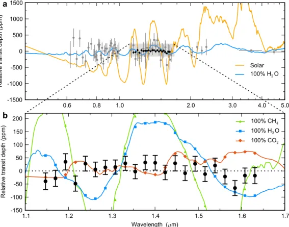
0.6 0.8 1.0 2.0 3.0 4.0 5.0 -1500 -1000 -500 0 500 1000 1500 Re lat ive tra nsi t d ep th (pp m) Solar 100% H2O 1.1 1.2 1.3 1.4 1.5 1.6 1.7 Wavelength (µm) -150 -100 -50 0 50 100 150 200 Re lat ive tra nsi t d ep th (pp m) 100% CH100% H2O4 100% CO2 a b
Figure 2: The transmission spectrum of GJ 1214b. a, Transmission spectrum measurements from our data (black points) and previous work (gray points)7–11, compared to theoretical models
(lines). The error bars correspond to 1σ uncertainties. Each data set is plotted relative to its mean.
Our measurements are consistent with past results for GJ 1214 using WFC310. Previous data rule
out a cloud-free solar composition (orange line), but are consistent with a high-mean molecular weight atmosphere (e.g. 100% water, blue line) or a hydrogen-rich atmosphere with high-altitude clouds. b, Detail view of our measured transmission spectrum (black points) compared to high mean molecular weight models (lines). The error bars are 1σ uncertainties in the posterior
distri-bution from a Markov chain Monte Carlo fit to the light curves (see the Supplemental Information for details of the fits). The colored points correspond to the models binned at the resolution of the observations. The data are consistent with a featureless spectrum (χ2
= 21.1 for 21 degrees of freedom), but inconsistent with cloud-free high-mean molecular weight scenarios. Fits to pure water (blue line), methane (green line), carbon monoxide (not shown), and carbon dioxide (red line) models haveχ2
= 334.7, 1067.0, 110.0, and 75.4 with 21 degrees of freedom, and are ruled
C lo u d t o p p re ssu re (mb a r) 0.0001 0.001 0.01 0.1 1 10 100 1000 Po st e ri o r p ro b a b ili ty d e n si ty (n o rma lize d ) 0 0.1 0.2 0.3 0.4 0.5 0.6 0.7 0.8 0.9 1 2.32 2.4 3 5 7 1013 1617 17.9 17.99 17.999
Mean molecular weight
0.01 0.1 1 10 25 50 75 90 99 99.9 99.99
Water mole fraction (%)
Figure 3: Spectral retrieval results for a two-component (hydrogen/helium and water) model
atmosphere for GJ 1214b. The colors indicate posterior probability density as a function of water
mole fraction and cloud top pressure. Black contours mark the 1, 2, and 3σ Bayesian credible
regions. Clouds are modeled with a gray opacity, with transmission truncated below the cloud altitude. The atmospheric modeling assumes a surface gravity of 8.48 m/s2 and an equilibrium temperature equal to 580 K.
Supplementary Information
The supplementary information describes the observations, data reduction, systematics cor-rection, and light curve fitting for transit observations of the super-Earth GJ 1214b.
Observations
We observed 15 transits of the super-Earth exoplanet GJ 1214b with the Wide Field Camera 3 (WFC3) instrument on the Hubble Space Telescope (HST) between UT 27 September 2012 and 20 August 2013. Each transit observation (or visit) consisted of four 96-minute HST orbits of time series spectroscopy, with 45-minute gaps in data collection in each orbit due to Earth occultation. We employed the G141 grism, which covers the wavelength range 1.1 to 1.7µm. The spectra were
binned at resolution R ≡ λ/∆λ ∼ 70. To optimize the efficiency of the observations, we used spatial scan mode, which moves the spectrum perpendicular to the dispersion direction during the exposure. Spatial scanning enables longer exposures for bright targets that would otherwise saturate, such as GJ 1214. We used a 0.12”/second scan rate for all exposures, which yielded peak per pixel counts near 23,000 electrons (30% of saturation). An example raw data frame is shown in Extended Data Figure 1.
0 50 100 150 200 250 Spectral pixel 0 50 100 150 200 250 Sp at ia l p ixe l 0.0 0.5 1.0 1.5 2.0 2.5 3.0 Ph ot oe le ct ro ns (× 10 4)
Extended Data Figure 1: An example spatially scanned raw data frame. The exposure time was
88.4 s.
The observations had the following design. At the beginning of each orbit, we took a direct image with the F130N narrowband filter to establish a wavelength zero-point. For the remainder of each orbit, we took spatially scanned exposures with the G141 grism. Each observation used
SPARS10, NSAMP=13 readout mode and scanned in the forward direction only. Each exposure contains NSAMP non-destructive reads. For transit observations 6 – 15, we modified our approach to reduce overhead time: we increased the exposure time to 103.1 s using the mode SPARS10, NSAMP=15, and scanned successively forward and backward. These approaches yielded 67 and 75 spectra per visit with duty cycles of 58% and 76%, respectively. One transit observation (UT 12 April 2013) was unsuccessful because the Fine Guidance Sensors failed to acquire the guide stars. We do not use data from this observation in our analysis. We also exclude data from the transit observations on UT 4 August 2013 and UT 12 August 2013, which showed evidence for a starspot crossing. Our final analysis therefore used 12 transit observations.
Data reduction
Our data reduction process begins with the “ima” data product from the WFC3 calibration pipeline,calwf3. These files are bias- and dark current-subtracted and flagged for bad pixels. For spatially scanned data, each pixel is illuminated by the stellar spectrum for only a small fraction of the exposure; the remainder of time it collects background. To aid in removing the background, we form subexposures of each image by subtracting consecutive non-destructive reads. A subex-posure thus contains photoelectrons gathered during the 7.4 s between two reads. We reduce each subexposure independently, as follows. First we apply a wavelength-dependent flat field correc-tion. Next we mask bad pixels that have been flagged data quality DQ = 4, 32, or 512 bycalwf3. To estimate the background collected during the subexposure, we draw conservative masks around all stellar spectra, measure the background from the median of the unmasked pixels, and subtract it. We compute a variance for the spectrum accounting for photon shot noise, detector read noise, and uncertainty in the background estimation.
We next correct for the wavelength dependence of the spectrum on detector position. The grism dispersion varies along the spatial direction of the detector, so we calculate the dispersion solution for each row in the subexposure and interpolate the photoelectron counts in that row to the wavelength scale corresponding to the direct image position. This interpolation also corrects bad pixels. We then create a 40-pixel tall extraction box centered on the middle of the spatial scan and extract the spectrum with an optimal extraction routine. Because each row has been interpolated to a common wavelength scale, the final spectrum is constructed by summing by column the spectra from all the subexposures. The unit of time sampling in the light curve is thus a single exposure, which is the sum of 12 subexposures. See Extended Data Figure 2 for an example extracted spectrum.
Finally, we account for dispersion-direction drift of the spectra during each visit and between visits. Using the first exposure of the first visit as a template, we determine a shift in wavelength-space that minimizes the difference between each subsequent spectrum and the template. The best-fit shift values are less than 0.1 pixel, both within each visit and between visits. We interpolate each spectrum to an average wavelength scale, offset from the template by the mean of the estimated wavelength shifts. This step does not have a significant effect on our results. We bin the spectra
1.0 1.1 1.2 1.3 1.4 1.5 1.6 1.7 1.8 Wavelength (µm) 1 2 Ph oto ele ctro ns ( × 10 6)
Extended Data Figure 2: An example extracted spectrum for an 88.4 s exposure. The dotted lines
indicate the wavelength range over which we measure the transmission spectrum.
in 5-pixel-wide channels, obtaining 29 spectroscopic light curves covering the wavelength range 1.05 – 1.70µm. The data near the edges of the grism response curve exhibit more pronounced
systematics, so we restrict our analysis to 22 spectroscopic channels between 1.15 and 1.63µm.
The limits are shown in Extended Data Figure 2.
Systematics correction
The light curves exhibit a ramp-like systematic similar to that seen in other WFC3 transit spec-troscopy data10,18,19. The ramp has a larger amplitude and a different shape in the first orbit com-pared to subsequent orbits, so we exclude data from the first orbit in our light curve fits, following standard practice. We correct for systematics in orbits 2 – 4 using two methods:
Method 1: model-ramp
This method fits an analytic model to the light curve10
. The model has the form:
M(t) = M0,λ(t)[Cλes+ Vλetv][1 − Rλeoe−tb/τλ] (1)
whereM0,λ(t) is the model for the systematics-free transit light curve, t is a vector of observation times, tvis a vector with elementstv,i equal to the time elapsed since the first exposure in the visit corresponding to timeti, tb is a vector with elementstb,i equal to the time elapsed since the first exposure in the orbit corresponding to time ti, Cλes is a normalization, Vλe is a visit-long slope, Rλeo is a ramp amplitude, andτλis a ramp timescale. The subscriptsλ, e, s, and o denote whether a parameter is a function of wavelength, transit epoch, scan direction, and/or orbit number, respectively.
Method 2: divide-white
The second method assumes the systematics are wavelength-independent and can be modeled with a scaled time series vector of white light curve systematics, denoted Z(t)18,20
. We fit the white light curveW (t) with themodel-ramptechnique to determineZ(t):
Z(t) = W (t)/M0(t), (2)
where M0(t) is the best-fit model to the white light curve. An example white light curve fit, including theZ vector, is shown in Extended Data Figure 3.
2.30 2.31 2.32 2.33 2.34 Ph oto ele ctro ns ( × 10 8) a 0.985 0.990 0.995 1.000 Re lat ive flu x b
Orbital phase (minutes) −200 0 200 O - C (p pm) c rms = 70 ppm −200 −150 −100 −50 0 50 100 Orbital phase (minutes)
2.336 2.338 2.340 Z ( × 10 8) d
Extended Data Figure 3: a, The broadband light curve from the first transit observation. b, The
broadband light curve corrected for systematics using the model-ramptechnique (points) and the best-fit model (line). c, Residuals from the white light curve fit. d, The vector of systematics
Z used in thedivide-whitetechnique.
The spectroscopic light curvesSλ(t) are modeled as
whereS0,λ(t) is the systematics-free transit light curve model for a given wavelength channel and Cλes is a normalization constant. We observe that the systematics have similar amplitude and form across the wavelength range of our observations, hence the viability of thedivide-white
technique. The dominant systematics in our data are related to persistence, which depends on the peak per pixel fluence19, but as can be seen in Extended Data Figure 2, the product of the stellar spectrum and the G141 grism response is nearly uniform over the 1.1 – 1.7µm range.
Light curve fits
We fit the spectroscopic light-curves with both thedivide-whiteandmodel-rampmethods and determined the best-fit parameters and errors with a Markov chain Monte Carlo (MCMC) algorithm. We divided the light curves into 19 data sets (12 visits, with 2 data sets for 7 of the visits), separated by transit epoch and spatial scan direction, to account for a normalization offset between the forward-scanned and reverse-scanned light curves. We fit the data sets in each spectral channel with five105
step MCMC chains, with2.5 × 104
burn-in steps removed from each chain. We tested for convergence using the Gelman-Rubin diagnostic. The results reported are from the five chains combined.
We analyzed each spectral channel independently. The free parameters for the
divide-whitefit are a normalization constantCλes, a linear limb darkening parameteruλ, and the planet-to-star radius ratio Rp/Rs,λ,e. Themodel-ramp fit had these same free parameters, plus an additional visit-long slope parameterVλe, ramp amplitudesRλeo, and a ramp timescaleτλ. We constrained the ramp amplitudes for orbits 3 and 4 to be equal within each data set. For both methods, we held the following orbital parameters fixed at the best-fit values for the white light curve: inclinationi = 89.1◦, the ratio of the semi-major axis to the stellar radius a/R
s = 15.23,
the orbital period P = 1.58040464894 days, and the time of central transit Tc = 2454966.52488 BJDTDB. We assume a circular orbit. There were a total of 32 and 67 free parameters per channel for thedivide-whiteandmodel-rampfits, respectively. The priors for each free parameter were uniform. We checked that the light curves are sufficiently precise to fit for all the free param-eters by visually inspecting pairs plots for the fit paramparam-eters. As an example, we show the posterior distributions of the parameters for the divide-whitefit of the 1.40 µm channel in Extended
Data Figure 4, and note that there is little correlation between parameters.
We report the measured transit depths, limb darkening parameters, and χ2
ν values for both
thedivide-whiteandmodel-rampmethods in Extended Data Table 1. The transit depths
given are the weighted averages over all epochs, minus the mean transit depth over all channels (0.013490 for divide-white and 0.013489 for model-ramp). For the results given in the main text, we use the divide-whitespectrum because the light curve fits from this method have fewer free parameters and lowerχ2
ν values.
1. We verified that the transmission spectra obtained with the divide-white and
model-rampmethods are consistent within 1σ, and that the main conclusions of the paper
are not affected by which method we chose.
2. We confirmed that the measured transit depths are consistent from epoch to epoch, as shown in Extended Data Figure 5. As a test, we fit separate transit depths to the forward- and reverse-scanned data, and found that the transit depths are consistent for the two scan direc-tions.
3. We tested the effects of using an inaccurate white light curve model (M0) for the
divide-whitemethod and found that the results are robust to changes inM0. For exam-ple, changing the model transit depth by 5σ from the best-fit white light curve value affects
the relative spectroscopic transit depths by less than 1 ppm.
4. We compare our results to the previously published WFC3 transmission spectrum for GJ 1214b10. Our relative transit depths are within 1σ for 18 wavelength channels and within
2σ for the other four channels. The 2 σ differences are not clustered in wavelength.
We also considered the effects of stellar activity on the transmission spectrum and found that it does not impact our results. The measured transit depths are consistent over all epochs in the white light curve and the spectroscopic light curves, which suggests that the influence of stellar activity on the spectrum is minimal. To confirm this, we simulated the effect of star spots8assuming
they are 300 K cooler than the 3250 K stellar photosphere22, and find that their influence is below our measurement precision. We also considered the possibility that the star spots have excess water due to their cooler temperature. This could introduce a water feature in the transmission spectrum, but it would not cancel out water features from the planet’s atmosphere. Given that we do not see evidence for water absorption in the spectrum, any contribution from water in unocculted star spots must be below the level of precision in our data. As a check, we computed the transmission spectrum from three transits occurring over a timespan of just two weeks, during which time the spot coverage should be roughly constant. Even with just these three transits, we rule out a pure H2O atmosphere at > 5 σ confidence, which confirms that any noise introduced by unocculted spots does not change our conclusion.
The derived limb darkening coeffients are shown in Extended Data Figure 6. We fit a single limb darkening coefficient to each channel and constrained the value to be the same for all the transits. Our limb darkening fits illustrate the importance of careful treatment of limb darkening for cool stars. There is a peak in the coefficients near1.45 µm that is due to the presence of water
in the star. As a result of this, fixing the limb darkening coefficients to a constant value in all spectral channels introduces a spurious water feature in the transmission spectrum. However, we can fit the limb darkening precisely with our data and it is non-degenerate with the transit depth. The uncertainty in our limb darkening fits introduces an uncertainty in the transit depth of less then 1 ppm. To confirm that fitting a linear limb darkening parameter is appropriate for our data, we
simulated a data set using a model water vapor atmosphere, quadratic limb darkening coefficents from a 3250 K stellar model, and the residuals and systematics from the real data. We analyze this mock data set in the same way we treat the real data and find that we fully recover the water vapor transmission spectrum with a single limb darkening parameter.
Transit depth (Rp/Rs)2(%) 0.23 0.26 0.29 0.32 Limb darkening u 1.3 1.34 1.38 0.9998 1.0 1.0002 0.23 0.26 0.29 0.32 0.9998 1.0 1.0002 Normalization C
Extended Data Figure 4: The posterior distributions for thedivide-whitefit parameters for
the 1.40µm channel from the first transit observation. The diagonal panels show histograms of
the Markov chains for each parameter. The off-diagonal panels show contour plots for pairs of parameters, with lines indicating the 1, 2, and 3σ confidence intervals for the distribution. The
Table 1: Derived parameters for the light curve fits for the divide-white (d-w) and model-ramp(m-r) techniques
Wavelength (µm) Transit Depth (ppm) Limb Darkening χ2
ν d-w m-r d-w m-r d-w m-r 1.135 − 1.158 −39 ± 31 6 ± 33 0.27 ± 0.01 0.28 ± 0.01 1.12 1.20 1.158 − 1.181 −28 ± 30 12 ± 32 0.26 ± 0.01 0.27 ± 0.01 1.01 1.24 1.181 − 1.204 34 ± 30 29 ± 30 0.25 ± 0.01 0.26 ± 0.01 1.04 1.44 1.205 − 1.228 −48 ± 28 −32 ± 29 0.26 ± 0.01 0.28 ± 0.01 0.90 1.22 1.228 − 1.251 27 ± 28 25 ± 29 0.26 ± 0.01 0.28 ± 0.01 0.85 1.29 1.251 − 1.274 5 ± 27 −6 ± 29 0.26 ± 0.01 0.26 ± 0.01 0.97 1.29 1.274 − 1.297 13 ± 27 12 ± 27 0.23 ± 0.01 0.23 ± 0.01 1.00 1.50 1.297 − 1.320 14 ± 26 0 ± 27 0.23 ± 0.01 0.25 ± 0.01 0.96 1.38 1.320 − 1.343 29 ± 26 2 ± 28 0.26 ± 0.01 0.27 ± 0.01 1.08 1.52 1.343 − 1.366 −2 ± 27 −15 ± 28 0.30 ± 0.01 0.32 ± 0.01 0.99 1.44 1.366 − 1.389 32 ± 27 35 ± 26 0.28 ± 0.01 0.29 ± 0.01 0.97 1.42 1.389 − 1.412 31 ± 27 33 ± 28 0.28 ± 0.01 0.29 ± 0.01 0.96 1.39 1.412 − 1.435 −5 ± 27 −33 ± 28 0.29 ± 0.01 0.31 ± 0.01 1.15 1.51 1.435 − 1.458 29 ± 29 17 ± 28 0.29 ± 0.01 0.30 ± 0.01 1.01 1.39 1.458 − 1.481 −8 ± 28 1 ± 29 0.32 ± 0.01 0.33 ± 0.01 1.01 1.33 1.481 − 1.504 27 ± 28 28 ± 28 0.28 ± 0.01 0.29 ± 0.01 0.94 1.37 1.504 − 1.527 −11 ± 28 −23 ± 29 0.27 ± 0.01 0.29 ± 0.01 1.15 1.58 1.527 − 1.550 20 ± 28 1 ± 29 0.27 ± 0.01 0.29 ± 0.01 1.17 1.56 1.550 − 1.573 −21 ± 28 0 ± 28 0.28 ± 0.01 0.29 ± 0.01 1.20 1.62 1.573 − 1.596 −65 ± 28 −62 ± 30 0.26 ± 0.01 0.28 ± 0.01 1.08 1.46 1.596 − 1.619 −17 ± 28 −6 ± 29 0.26 ± 0.01 0.27 ± 0.01 1.34 1.69 1.619 − 1.642 −17 ± 30 −26 ± 30 0.22 ± 0.01 0.24 ± 0.01 1.16 1.59
-2000 200 1.15µm -2000 200 1.17µm -2000 200 1.19µm -2000 200 1.22µm -2000 200 1.24µm -2000 200 1.26µm -2000 200 1.29µm -2000 200 1.31µm -2000 200 1.33µm -2000 200 1.35µm 1 3 5 7 9 11 Transit number -2000 200 Re lat ive tra nsi t d ep th (pp m) 1.38µm 1.40µm 1.42µm 1.45µm 1.47µm 1.49µm 1.52µm 1.54µm 1.56µm 1.58µm 1.61µm 1 3 5 7 9 11 1.63µm
Extended Data Figure 5: Transit depths relative to the mean in 22 spectroscopic channels, for the
1.1 1.2 1.3 1.4 1.5 1.6 1.7 Wavelength (µm) 0.20 0.22 0.24 0.26 0.28 0.30 0.32 0.34 0.36 Limb da rke nin g co eff ici en t 3026 K 3156 K 3250 K 3350 K 3450 K
Extended Data Figure 6: Fitted limb darkening coefficients as a function of wavelength (black
points) and theoretical predictions for stellar atmospheres with a range of temperatures (lines). The uncertainties are 1σ confidence intervals from an MCMC. The temperature of GJ 1214 is estimated