HAL Id: hal-01105398
https://hal.archives-ouvertes.fr/hal-01105398
Submitted on 20 Jan 2015HAL is a multi-disciplinary open access archive for the deposit and dissemination of sci-entific research documents, whether they are pub-lished or not. The documents may come from teaching and research institutions in France or abroad, or from public or private research centers.
L’archive ouverte pluridisciplinaire HAL, est destinée au dépôt et à la diffusion de documents scientifiques de niveau recherche, publiés ou non, émanant des établissements d’enseignement et de recherche français ou étrangers, des laboratoires publics ou privés.
Upscaling and large-scale modeling of the dissolution of
gypsum cavities
Jianwei Guo, Michel Quintard, Farid Laouafa
To cite this version:
Jianwei Guo, Michel Quintard, Farid Laouafa. Upscaling and large-scale modeling of the dissolution of gypsum cavities. The 25th International Symposium on Transport Phenomena, Nov 2014, Krabi, Thailand. �hal-01105398�
To cite this version : Guo, Jianwei and Quintard, Michel and Laouafa, Farid
Upscaling and large-scale modeling of the dissolution of gypsum cavities. In:
The 25th International Symposium on Transport Phenomena, 5 November
2014 - 7 November 2014 (Krabi, Thailand).
O
pen
A
rchive
T
OULOUSE
A
rchive
O
uverte (
OATAO
)
OATAO is an open access repository that collects the work of Toulouse researchers
and makes it freely available over the web where possible.
This is an author-deposited version published in:
http://oatao.univ-toulouse.fr/
Eprints ID : 12166
Any correspondance
concerning this service should be sent to the repository
UPSCALING AND LARGE-SCALE MODELING OF THE DISSOLUTION OF GYPSUM CAVITIES
Jianwei Guo1, Michel Quintard1, 2 and Farid Laouafa3
1 Université de Toulouse; INPT, UPS; IMFT (Institut de Mécanique des Fluides de Toulouse), 31400 Toulouse, France 2 CNRS; IMFT; 31400 Toulouse, France
3 Institut National de l’Environnement Industriel et des Risques, 60550 Verneuil-en-Halatte, France
ABSTRACT
The dissolution of geological formations containing gypsum can rapidly create various karstic features, and may potentially generate great risks such as subsidence and collapse. To understand the gypsum dissolution mechanism is very important to develop safety measures. In practical applications, it is not feasible to take into account all the pore-scale details at a large-scale by direct numerical modeling, therefore some sort of macro-scale modeling is necessary. In this study, we will develop a general expression of the macro-scale model for gypsum dissolution, starting from the pore-scale transport problem with boundary condition of thermodynamic equilibrium or non-linear reaction, making use of the method of volume averaging. Then, this macro-scale porous medium model will be used as a diffuse interface model (DIM) to solve for large-scale cavity dissolution examples, typical of situations leading to sinkhole formations, with the mass exchange term for Ca2+ given in the form of a first order
reaction. A work-flow is proposed to choose properly the parameters in the model to reflect accurately the interface recession. Additional tests are performed to check which type of momentum balance equation should be used. It is shown that a proper choice for the mass exchange coefficient leads to satisfactory results with the macro-scale model, and that Darcy-Darcy and Darcy-Navier-Stokes formulations give almost the same cavity formation for the studied cases.
INTRODUCTION
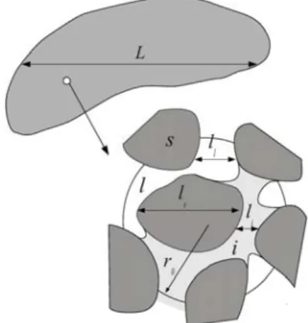
Dissolution of gypsum cavities are found in many fields, such as karst formation, aquifer evolution, and dam stability (1)(2), etc. It causes concern because of the potential to raise some undesirable effects, for instance collapse and subsidence. The understanding of dissolution processes is a crucial issue for effective planning control and engineering practice. The mass and momentum transport in the dissolution process often happens in a hierarchical, multi-scale system, as schematically depicted in Fig. 1. In such a system with multi-scale aspects, taking into account all the pore-scale details at a large-scale is inaccessible by direct numerical simulations (DNSs). To describe the dissolution of gypsum which is contained in a porous formation, it is essential to develop some sort of macro-scale models. Such a macro-scale porous medium model can also serve as a diffuse interface model to describe the dissolution at a fluid-solid interface, as done in (3)(4). In the developed macro-scale model, effective properties are generally employed to represent the averaged behaviors of the micro-scale features and various related studies can be found in the literature. An overview
of dispersion in porous media with and without reaction has been presented by Rudraiah and Ng (5).
Figure 1. Multi-scale description of the dissolution system
Regarding developments associated to the upscaling of dissolution problems, in (6) and (7), equilibrium or non-equilibrium macro-scale models for thermodynamic dissolution with a Dirichlet condition were obtained, neglecting contributions of the interface velocity in the closure problems. In (8), the authors solved the case of mass exchange controlled by partitioning expressions (Raoult's law, Henry's law, etc...), and they took into account the interface velocity in the closure problems for this particular case. The case of first-order reaction rate has been studied by Whitaker (9) and Valdés-Parada et al. (10).
Concerning numerical investigation on gypsum cavities, studies are scarce. Some examples are available for gypsum dissolution, Rehrl et al. (11) simulated a conduit development under artesian conditions, by analyzing the variations of conduit diameters and hydraulic heads at different stages, with a continuum-pipe flow model. To our knowledge, few papers have been published on the large-scale gypsum dissolution model or the numerical simulation for gypsum cavity evolution with a moving interface.
Given this research background, the objectives of this study are: (i) to develop the general forms of the gypsum dissolution macro-scale model, starting from pore-scale problems with thermodynamic, or nonlinear reactive boundary conditions, and taking into account the role of interface velocity, (ii) to implement numerical simulations with COMSOL® to solve for large-scale cavity dissolution
examples, typical of situations leading to sinkhole formations.
PORE-SCALE MODEL
As schematically illustrated in Fig. 1, the porous medium under consideration consists of three phases at the pore-scale: two solid phases, one being soluble (gypsum), denoted s, the other insoluble, denoted i, and a liquid phase (water + dissolved species), denoted l.
We adopt in this paper the assumption that gypsum dissolution can be described by the dissolution of a pseudo-gypsum water component. For convenience, and for the purpose of future introduction in more complex geochemistry models, we choose to follow the ion Ca2+.
The pore-scale problem under consideration corresponding to the mass and momentum transfer of calcium is described by the following equations
in Vl (1)
in Vl (2)
where, ρl is the liquid density, vl is the liquid velocity, ωl is
the mass fraction of Ca2+ and D
l is the molecular diffusion
coefficient.
One must be reminded that these equations can be potentially simplified greatly if one assumes that is a constant. If necessary, Boussinesq's approximation may be introduced to evaluate the potential for natural convection and this should be accurate enough.
The boundary conditions for Ca2+ mass balance at the
interface with the solid phase may be written as a kinetic condition following
at Als (3)
where, nls is the normal vector pointing from the liquid
towards the solid, wsl is the solid-liquid interface velocity, MCa is the molar weight of Ca2+, k
s is the surface reaction
rate constant, ωeq is the equilibrium mass fraction of Ca2+, n is the order of the chemical reaction, ρs is the solid density, ωs is the mass fraction of Ca2+ in Vs and Als
denotes the solid-liquid interface.
Mass balance for the solid phase gives the following boundary condition
at Als (4)
where Mg is the molar weight of gypsum and we have νs=Mg/MCa.
The total mass balance boundary condition may be written formally as
(5)
which can be used to calculate the liquid velocity.
For computational purposes, it is convenient to express the diffusive flux at the surface approximately as
(BC I)
(6) which neglected the interface velocity since it is only on the order of 10-3.
In the above, we talked about the case of a reactive boundary condition, while when the solid-liquid interface is under thermodynamic equilibrium, the boundary condition can be described as
(BC II) (7)
which is the limit of the reactive condition for large Damkhöler numbers.
The problem has to be completed with momentum balance equations: Navier-Stokes equations for instance. Assuming that and are constants, and that the velocity of dissolution is small compared to the relaxation time of the viscous flow, the problem for the momentum balance equations is independent of the concentration field and, therefore, can be treated independently. Hence, one may readily assume that the macro-scale momentum equations has any type suitable for the flow conditions under consideration, i.e., Darcy's law, etc... Consequently, we can focus on the transport problem assuming that , and its average value, is a known field.
UPSCALING
To develop an upscaled model, several methods can be adopted, for instance, volume averaging (12), moments matching (13) and multi-scale asymptotics (14). In this present study, we choose to follow the developments of a macro-scale model based on the method of volume averaging. The general framework has been developed over several decades and a comprehensive presentation can be found in (12).
As defined in Fig. 1, the corresponding micro-scale (pore-scale) characteristic lengths are defined as ll, ls and li
respectively, and the macro-scale characteristic length is denoted L. In addition, a third length scale, the so-called support scale, r0 in this study, is associated with the
representative volume. A fundamental hypothesis which should be kept in mind to perform volume averaging is that, in terms of length scales, we have ll, ls and li «r0 «L.
Averages are defined in the traditional manner so the superficial average velocity gives
(8)
where Ul is the intrinsic average velocity and is the
porosity.
The intrinsic average mass fraction is defined as
(9)
We introduce the following deviation fields
, (10) , (11) By applying Eqs. (10) , (11) to the pore-scale problem, we can obtain a set of problem for . However, at this stage, the problem is still a coupling of different scales which is difficult to solve. To develop a closed form of the problems, we propose the following approximate solution for the coupled solution of the macro-scale and micro-scale governing equations for and ,
(12) where, sl and bl are called the closure variables.
Neglecting terms involving or higher derivatives, collecting terms for and and then applying the fundamental lemma, we obtain two sets of “closure problems” for sl and bl respectively.
In order to solve the closure problems, we must know the interface position and velocity, as well as the macro-scale concentration because of the reaction non-linearity. We are faced here with the classical geochemistry problem, and, in principle, we must solve the coupled pore-scale (here the closure problems) and macro-scale equations at each time step in order to compute the interface evolution and . In geochemistry (or other problems involving changing geometries) it is often assumed a given interface evolution and the closure problems are solved for each realization, which in turn yields effective properties dependent on, for instance, the medium porosity. In turn, these effective properties can be used in a macro-scale simulation without the need of a coupled micro-scale/macro-scale solution. Of course, it is well known that some history effects are lost in this process, but it has the advantage that this is far more practical than solving the coupled problem. We will not discuss further this difficulty which is well known when solving dissolution or crystallization problems.
If we assume that mass fluxes near the interface are triggered by the diffusive flux, which in the case of gypsum is consistent with some quantitative analysis, we may develop approximate closure problems.
The closure problems can be developed following ideas available in the literature, see (6)(8)(10) for the full deduction of the upscaling procedure, and we present only the final macro-scale equations for the mass balance,
which gives
(13) with the dispersion tensor, the non-traditional effective velocity and the mass exchange term given by
(14)
(15)
and
(16)
respectively, where the effective reaction rate coefficient and the additional gradient term coefficient are given by
(17) and
(18)
One must remember that the macro-scale problems involve also the following averaged equations
and
(19)
(20)
with the relation
(21)
All the effective parameters mentioned above can be obtained by solving closure problems for sl and bl.
The averaging of the momentum equation would have led to a macro-scale equation, for instance Darcy's law expressed as
(22)
where the liquid permeability Kl will depend on the
dissolution history. As a classical geochemistry approximation, we will assume it depends, like the other effective parameters, on the volume fractions, in our case we will have .
The macro-scale equations for the case with thermodynamic equilibrium boundary condition at pore-scale are the same as before, but for a different expression of the mass exchange term which can be written as
(23) where we have adopted the following notation for the mass exchange coefficient
(24)
and the additional gradient term
(25)
In order to understand the effective macro-scale model developed above, we are interested in getting solutions for the longitudinal dispersion coefficient, (Dl*)xx, and the
effective reaction rate coefficient, ks,eff, for the case with
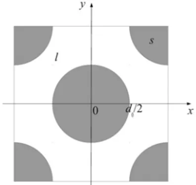
non-linear reactive boundary conditions for the 2D problem. The geometry of a representative unit cell is depicted in Fig. 2 and it is only composed of s- and l- phase. The problem under consideration is assumed at steady-state, and the variation of the liquid density is negligible.
Figure 2. 2D geometry of the unit cell
As the reaction order for gypsum dissolution is ranging
from 1 to 4.5 at different stages, in the following numerical simulations, we will test for n=[1, 3, 5]. The porosity is about 0.37 hereby and after. The velocity field is obtained by solving Navier-Stokes equations with Re=10-6, in which condition the inertia effects are
negligible. The Reynolds number is defined as
(26)
with the characteristic length defined as the diameter of the solid phase, lr=d0, and the characteristic velocity is
defined as the intrinsic average of the component of the velocity in the x-direction, .
Since we solve the closure problems in a dimensionless form, we define two more important parameters, the pore-scale Damkhöler and Péclet numbers as
(27)
(28)
The numerical simulations are performed with COMSOL®. The first parameter to be discussed is the
longitudinal dispersion coefficient in terms of (Dl*)xx/Dl. It
can be written in a classical form as
(29) As presented in Fig. 3, (Dl*)xx/Dl is smaller than 1 at
small Pe, which is the result of the tortuosity effects. The impact of Da is dependent on the Pe value. When Pe<20, (Dl*)xx/Dl increases with Da, while after a transition zone, a
large Da will lead to a smaller (Dl*)xx/Dl when Pe>30. This
reversed effect of Da is consistent with the results reported in (10) for the linear case.
In addition to Pe and Da, the reaction order is also playing a role. One may observe from Fig. 3 that for small Pe with Da=1, (Dl*)xx/Dl increases with n, while for large
Pe with Da=100, (Dl*)xx/Dl decreases with n.
Another parameter under investigation is the effective reaction rate coefficient ks,eff. In Fig. 4, we plot ks,eff/ks
versus Da for Pe=1 and Pe=10. One sees from the figure that whatever the value of Pe and n, ks,eff/ks is equal to
about 1 at small Da. At this stage, the dissolution process is limited by the nonlinear reaction, so the effective reaction rate coefficient is the same as the pore-scale reaction rate coefficient. With the increase of Da, mass transport becomes a limiting mechanism and the ratio
ks,eff/ks tends to decrease until it reaches another constant,
about zero, at very large Da. One should note that with the increase of Da, ks,eff will increase with ks, and when the
Da, i.e., ks, tends to become infinitely large, ks,eff stops
growing and the ratio ks,eff/ks is consequently rather small.
Actually, in the case of a large Da, the boundary condition will become thermodynamic equilibrium and the mass exchange coefficient should be predicted by Eq. (24) instead of Eq. (17).
Regarding the impact of Pe and n, for linear reactive case or the case with larger Pe, the decrease of ks,eff/ks is
delayed.
Some additional numerical tests were performed to see the accuracy of this macro-scale model. The comparison between the results obtained by the DNSs and this macro-scale model agree very well, leading to an error smaller than 1%, for Pe and Da in the range [0.001,100].
Figure 3. (Dl*)xx/Dl as a function of Pe
Figure 4. ks,eff/ks as a function of Da LARGE-SCALE MODELING
As stated previously, the macro-scale model developed for the porous medium can also employed as a diffuse interface model (DIM) for the case of solid dissolution. In this section, we are interested in implementing it for a large-scale cavity evolution example. The geometry is illustrated in Fig. 5, where subdomain d contains soluble gypsum (denoted s), insoluble material (denoted i), and a liquid phase (denoted l) which contains water and the dissolved gypsum. Subdomains a and e are composed only by the fluid phase and insoluble solid initially, with
different permeability and porosity. The geometric and physical parameters are presented in Table 1. With the injection of a fluid (water in this study) from the left boundary of subdomain a at a velocity of , solid gypsum in subdomain d will be dissolved and gradually create a cavity.
As there is insoluble materials in this studied case, we transformed the macro-scale model developed in the last section to a form suitable for this particular problem.
Mass balance of the liquid phase gives
(30)
Figure 5. Schematic description of the dissolution system Table. 1 Geometric features and physical properties Parameters Description Value Unit
w1 width of e1 3 m
w2 width of e2 3 m wd width of d 5 m
hed height of e and d 5 m
ha height of a 5 m
ɛa porosity of a 0.35 dimensionless
ɛe porosity of e 0.2 dimensionless
ɛ porosity of d 0.9 dimensionless
Mass balance of solid gypsum gives
(31) Mass balance of Ca2+ gives
(32) where
(33)
, (34), (35)
with and the volume fraction of the fluid and the solid gypsum respectively. We have the constraints that
, (36), (37) where is the volume fraction of the insoluble material.
The mass exchange of calcium gives
(38)
In fact, because dissolution may lead to a true cavity without the solid phase, we may use a modified version of Navier-Stokes equation in the dissolved region
(39) where is the fluid viscosity and is the so-called effective viscosity of the fluid, which is dependent on the porous medium property. In general, is heterogeneous due to the large variations of material properties, however, in practice it is often assumed that effective viscosity is homogeneous and that for simplification. If local Reynolds number is small, the role of inertial terms are negligible, and Equation (39) turns out to be the Brinkman-Darcy equation
(40)
When permeability is infinite we obtain Stokes' equation
(41) and when the permeability is small enough we have Darcy's law
(42)
We took
(43) for subdomain d
From Eqs. (30) and (31), we have
(44) For all three subdomains, the problems are in the same
form, except that for subdomains a and e
, , (45), (46), (47) In this study, we set a relatively small permeability
K0=10-15 m2 and a saturation of solid gypsum Sinitial=0.9 for
subdomain d. Besides, permeability for the dissolved region and for the undissolved region in subdomain d have the relation Kf »Kl . For a given inlet velocity V0=10-6
m s-1, we would like first to investigate the impact of K
f
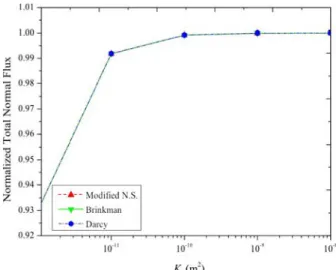
on the geometry and recession velocity of the dissolving surface, implementing three different equations, i.e., the modified Navier-Stokes equation, the Brinkman-Darcy equation and Darcy's law. In Fig. 6, we plot the normalized mass flux over the dissolving surface versus the cavity permeability, using different momentum equations. One sees that the mass flux over the dissolving surface increased dramatically when the permeability increased from 10-12 m2 by an order of 2. After the
permeability reached 10-10 m2, further increases lead to
only a negligible increase of the mass flux. We obtained nearly the same results with the modified Navier-Stokes equation and the Brinkman-Darcy equation for the whole range of Kf, and they behave a little differently from
Darcy's law when Kf is higher than 10-9 m2, with the
maximum difference of about 0.24%. We may conclude that the inertia term is not important in this study, while the viscous terms play a role when permeability is large enough (about 10-9 m2 in this case). We may conclude that:
•below a permeability of 10-9 m2, the cavity is not well
represented by any of the momentum equation,
•above this value, the modified Navier-Stokes or the Brinkman-Darcy equation gives the same result, which is a priori close to the physical one (i.e., the flow of a viscous fluid in a cavity),
•it is somehow surprising that a pure Darcy model, with a sufficiently large permeability in the cavity gives almost the same dissolving flux.
This latter remark is encouraging since Darcy equations are much easier to solve! However, a generalization of this result has to be taken with caution. Indeed, if we have a developing boundary layer over a flat surface, the Darcy Sherwood number along the boundary at a position x is given by
(48) if we have a small Schmidt number, this correlation is also the same in the case of a laminar Navier-Stokes flow. However, the Schmidt number for water is about
(49) which suggests that we should see a difference between Darcy and Navier-Stokes calculations. In addition, in the case of significant water density variations, we may have a departure from the classical boundary layer solution
because of buoyancy effects. Or this may also change because of different flow conditions (heterogeneities, roughnesses, etc...).
Figure 6. Normalized total normal flux over the dissolving surface as a function of cavity permeability To study the impact of α on the dissolution process, we carried out simulations with the macro-scale equations presented above. To investigate the characteristic time in such a case, we estimate the residual time approximately as
(50) and the dissolution time is about the inverse of α. Therefore, we need a relatively large α to reach rapidly the equilibrium concentration along the dissolving surface in order to have an actual boundary layer similar to the one with a sharp interface. However, α can not be infinite for simulation reasons. According to our numerical tests, α =10-5 s-1 is a good choice to get a satisfactory result with
DIM for the investigated problem (given the fact that dissolution is a very slow process here). The existence of the boundary layer induced the decrease of mass flux across the dissolving surface, from the entrance to the exit, which further caused the lower dissolution velocity in the exit region (cf. Fig. 7(c)).
As stated above, the dissolution velocity is somehow difficult to capture with DIM, due to the required very fine mesh, a relatively large α and the artificial tweak of Kf .
Therefore, we have to verify that the flux exchanged in the DIM between the solid and dissolved area is correct. Contrary to small-scale simulations, it is very difficult to carry on ALE simulation on a large cavity, so we used the modified Navier-Stokes equation with a fixed boundary but without dissolution, as an alternative way, to check that we have the correct concentration field and hence the correct dissolution velocity. The comparison of results obtained by different methods are illustrated in Fig. 7, from which we see that concentration fields agree very well with α =10-5 s-1.
(a) (b) (c)
(d) (e) (f)
(g) (h) (i)
Figure 7. Simulation results of normalized mass fraction Ωl/ωeq of dissolved gypsum (surface) and velocity (arrow)
fields at t=8×10⁹ s. (a) DIM with modified N.S. equations,
α =10-7 s-1;(b) DIM with modified N.S. Equations, α =10-6
s-1; (c) DIM with modified N.S. equations, α =10-5 s-1; (d)
DIM with Darcy' law, α =10-7 s-1; (e) DIM with Darcy'
law, α =10-6 s-1; (f) DIM with Darcy' law, α =10-5 s-1; (g)
case (a) with fixed boundary; (h) case (b) with fixed boundary; (i) case (c) with fixed boundary
CONCLUSION
In this paper we have presented an analysis of dissolution problem involving gypsum. Porous medium models have been obtained theoretically for the reactive and equilibrium cases. They have served as the basis of a DIM for subsequent use to model large-scale cavity dissolution.
Using the assumptions of a pseudo-component dissolving with an equilibrium boundary condition, numerical tools have been tested to solve for large-scale cavity dissolution problems, typically for an aquifer situation leading to potential sinkhole formation. Direct interface tracking, such as with ALE, was found to be very difficult to carry on. We proposed an alternate route using a DIM based on the porous medium theory. A work-flow was proposed to choose properly the parameters in the DIM model that would reproduce as accurately as possible the concentration field and fluxes and, consequently, the interface recession. Additional tests were performed to check which type of momentum balance equation should be used. It was found that Darcy-Darcy, Darcy-Brinkmann or Darcy-Navier-Stokes formulation give almost the same cavity formation.
NOMENCLATURE
Als solid-liquid interface, dimensionless
d0 diameter of the solid phase, m
Da pore-scale Damkhöler number, dimensionless Dl molecular diffusion coefficient, m2 s-1 Dl* dispersion tensor, m2 s-1
hl additional gradient term coefficient, mol m-1 s-1 ks surface reaction rate constant, mol m-2 s-1
ks,eff effective reaction rate coefficient, mol m-2 s-1
K permeability, m2
li, ll ,ls pore-scale characteristic lengths, m L macro-scale characteristic length, m
, mass exchange of gypsum, Ca2+, kg m-3 s-1
MCa, Mg molar weight of Ca2+, gypsum, g mol-1 n chemical reaction order, dimensionless
nls normal vector pointing from the liquid towards
the solid, dimensionless
Pe pore-scale Péclet number, dimensionless Re pore-scale Reynolds number, dimensionless
sl closure variable, dimensionless
S saturation, dimensionless
Ul intrinsic average velocity, m s-1 Ul* effective velocity, m s-1 vl pore-scale liquid velocity, m s-1 V0 inject velocity, m s-1
Vl superficial intrinsic average velocity, m s-1 wsl solid-liquid interface velocity, m s-1
α mass exchange coefficient, s-1
, volume fraction of fluid, solid gypsum fluid viscosity, Pa s
effective viscosity, Pa s ρl,, ρs liquid, solid density, kg m-3 ωeq equilibrium mass fraction of Ca2+
ωl, ωs mass fraction of Ca2+ in the liquid, solid phase
intrinsic average mass fraction, dimensionless
REFERENCES
(1) Waele, J. D., Plan, L. and Audra, P. (2009):" Recent developments in surface and subsurface karst geomorphology: An introduction".
Geomorphology, Vol.106, pp.1-8.
(2) Romanov, D., Gabrovšek, F. and Dreybrodt, W. (2003):" Dam sites in soluble rocks: a model of increasing leakage by dissolutional widening of
fractures beneath a dam". Engineering Geology, Vol.70, pp.17-35.
(3) Luo, H., Quintard, M., Debenest, G. and Laouafa, F. (2012):" Properties of a diffuse interface model basedon a porous medium theory for solid–liquid dissolution problems". Computational
Geosciences, Vol 16, pp. 913–932.
(4) Luo, H., Laouafa, F., Guo, J. and Quintard, M. (2014):" Numerical modeling of three-phase dissolution of underground cavities using a diffuse interface model". Int. J. Numer. Anal. Meth.
Geomech, DOI: 10.1002/nag.2274.
(5) Rudraiah, N., and Chiu-On Ng. (2007):" Dispersion in porous media with and without reaction: A review". Journal of Porous Media,Vol 10, pp. 219-248
(6) Quintard, M., and Whitaker, S. (1994):" Convection, dispersion, and interfacial transport of contaminant: homogeneous porous media".
Advances in Water Resources, Vol.17, pp.221-239.
(7) Golfier, F., Zarcone, C., Bazin, B., Lenormand, R., Lasseux D. and Quintard, M. (2002):" On the ability of a Darcy-scale model to capture wormhole formation during the dissolution of a porous medium". Journal of Fluid Mechanics, Vol.457, pp.213-254.
(8) Soulaine, C., and Debenest, G. and Quintard, M. (2011):" Upscaling multi-component two-phase flow in porous media with partitioning coefficient".
Chem. Eng. Sci., Vol.66, pp. 6180- 6192.
(9) Whitaker, S. (1986):" Transient diffusion, adsorption and reaction in porous catalysts: The reaction controlled, quasi-steady catalytic surface".
Chem. Eng. Sci., Vol.41, pp.3015- 3022.
(10) Valdés-Parada, F.J., Aguilar-Madera, C.G. and Álvarez-Ramírez, J. (2011):" On diffusion, dispersion and reaction in porous media". Chem.
Eng. Sci., Vol.66, pp. 2177 - 2190.
(11) Rehrl, C., Birk, S. and Klimchouk, A. B. (2008):" Conduit evolution in deep-seated settings: Conceptual and numerical models based on field observations". Water Resources Research, Vol.44. (12) Whitaker, S. (1999). The Method of Volume
Averaging. Kluwer Academic Publishers
(13) Shapiro, M. and Brenner, H. (1988):" Dispersion of a chemically reactive solute in a spatially periodic model of a porous medium". Chem. Eng. Sci., Vol.43, pp.551-571.
(14) Bensoussan, A., and Lions, J-L. and Papanicolau, G. (1978). Asymptotic Analysis for Periodic