Coordination and control of UAV fleets using mixed-integer linear programming

Coordination and Control of UAV Fleets using

Mixed-Integer Linear Programming

by

John Saunders Bellingham

Bachelor of Applied Science

University of Waterloo, 2000

Submitted to the Department of Aeronautics and Astronautics

in partial fulfillment of the requirements for the degree of

Master of Science in Aeronautics and Astronautics

at the

MASSACHUSETTS INSTITUTE OF TECHNOLOGY

September 2002

©

John Saunders Bellingham, MMII. All rights reserved.

The author hereby grants to MIT permission to reproduce

and distribute publicly paper and electronic copies

MASSACHUSETTS

_INSTITUTE

of this thesis document in whole or in part.

OFTECHNOLOGY

SEP

1 0 2003

LIBRARIES

A uthor... ..

...

Department of Aeronautics and Astronautics

August 9, 2002

C ertified by ... ...

...

...

Jonathan P. How

Associate Professor

Thesis Supervisor

Accepted by ....

...

Edward M. Greitzer

Professor of Aeronautics and Astronautics

Chair, Department Committee on Graduate Students

Coordination and Control of UAV Fleets using

Mixed-Integer Linear Programming

by

John Saunders Bellingham

Submitted to the Department of Aeronautics and Astronautics on August 9, 2002, in partial fulfillment of the

requirements for the degree of

Master of Science in Aeronautics and Astronautics

Abstract

This thesis considers two important topics in the coordination and control of fleets of UAVs; the allocation and trajectory design problems. The first allocates waypoints to individual vehicles in the fleet, and includes constraints on vehicle capability, waypoint visitation, and visit timing. Formulations of the allocation problem are presented to find minimum mission completion time and maximum stochastic expectation of mission benefit. The trajectory design problem provides a minimum time reference trajectory to the goal, while avoiding obstacles in the environment and obeying a limited turning rate.

Mixed-Integer Linear Programming (MILP) is applied to both problems in order to inte-grate discrete and continuous decisions, making into one optimization program. The MILP allocation program's cost function is evaluated using estimated trajectory parameters, which come from approximated paths. This partially decouples the allocation and trajectory design problems, and detailed trajectories can later be designed for the selected waypoint sequences. This significantly reduces the allocation solution time, with negligible loss in performance. The stochastic formulation is shown to recover sophisticated attrition reduction strategies.

MILP is applied to the trajectory design problem within a receding horizon control frame-work. The optimization uses a novel terminal penalty which approximates the cost to go to the goal, and is cognizant of intervening obstacles. This approach provides trajectories that are within 3% of optimal with significantly less computational effort, while avoiding entrapment in concave obstacles. This trajectory designer is modified to guarantee its sta-bility, and the resulting controller is capable of planning trajectories in highly constrained environments, without large increases in computation time.

The approaches presented here successfully solve the allocation and trajectory design problems, offering good performance and computational tractability.

Thesis Supervisor: Jonathan P. How Title: Associate Professor

Acknowledgments

This research was funded in part under DARPA contract

#

N6601-01-C-8075 and Air Force

Contents

1 Introduction

1.1 The UAV Trajectory Design Problem . . . .

1.1.1 Summary of Previous Work on UAV Trajectory Design

1.1.2 Outline of Trajectory Design Approach . . . .

1.2 The Allocation Problem . . . .

1.2.1 Summary Previous Work on the Allocation 1.2.2 Outline of Allocation Problem Approach

2 Receding Horizon Control Trajectory Design 2.1 Introduction . . . . 2.2 Fixed Horizon Minimum Time Controller . . . . 2.3 Simple Terminal Cost Formulation . . . . 2.4 Improved Receding Horizon Control Strategy . . 2.4.1 Control Architecture . . . . 2.4.2 Computation of Cost Map . . . .

2.4.3 Modified MILP Problem . . . .

2.5 R esults . . . . 2.5.1 Avoidance of Entrapment . . . . 2.5.2 Performance . . . . 2.5.3 Computation Savings . . . . 2.5.4 Hardware Testing Results . . . .

Problem 15 16 16 . . . . 18 . . . . - . - - 19 . . . . 21 . . . . 23 25 . . . . 25 . . . . 26 . . . . 28 . . . . 30 . . . . 30 . . . . 32 . . . . 35 . . . . 36 . . . . 36 . . . . 37 . . . . 38 . . . . 40

2.5.5 Planning with Incomplete Information . 2.6 _{Conclusions . . . .}

3 Stable Receding Horizon Trajectory Design 3.1 Review of Stability Analysis Techniques . . . . 3.2 Stable Receding Horizon Trajectory Designer

3.2.1 Terminal Constraint Set . . . . 3.2.2 The Tree of Trajectory Segments . . . .

3.2.3 Stability Analysis . . . .

3.3 MILP Formulation of Controller . . . . 3.3.1 Tangency Constraint . . . . 3.3.2 Selection of Unit Vectors in P . . . . . 3.3.3 Arc Length Approximation . . . . 3.3.4 Linearized Terminal Penalty . . . . 3.4 Simulation Results . . . . 3.4.1 Operation of the Trajectory Designer . . 3.4.2 Trajectory Design in Highly Constrained 3.4.3 Design of Long Trajectories . . . . 3.4.4 Rate of Decrease of Terminal Penalty 3.5 Conclusions .. .. .. ....

Environments

4 Minimum Time Allocation

4.1 Introduction . . . . 4.2 Problem Formulation _{. . . .}

4.3 The Allocation Algorithm . . . .

4.3.1 Overview . . . . 4.3.2 Finding Feasible Permutations and their Costs

4.3.3 Task Allocation . . . .

4.3.4 Modified Cost: Total Mission Time . . . .

8 41 45 47 . . . . 48 52 53 54 57 58 60 62 64 66 67 . . 67 . . 68 . 70 72 . . . . 73 75 75 76 78 78 79 82 83

. . . .

. . . .

4.3.5 Timing Constraints . . . .

4.4 Sim ulations . . . .

4.4.1 Simple Allocation Example . . . .

4.4.2 Large-Scale Comparison to Fully Coupled Approach . . . .

4.4.3 Complex Allocation Problem . . . .

4.5 C onclusions . . . .

5 Maximum Expected Score Allocation

5.1 Introduction . . . .

5.2 Optimization Program Formulations . . . .

5.2.1 Purely Deterministic Formulation . . . .

5.2.2 Deterministic Equivalent of Stochastic Formulation . . . .

5.2.3 Stochastic Formulation . . . .

5.3 R esults . . . .

5.3.1 Nominal Environment . . . . 5.3.2 High Threat Environments . . . . 5.3.3 Results on Larger Problem . . . .

6 Conclusions

6.1 Contributions to the Trajectory Design Problem . . . .

6.2 Contributions to the Allocation Problem . . . .

6.3 Future Work . . . . 84 85 85 86 89 90 93 93 94 95 97 98 103 103 104 104 109 109 110 111

List of Figures

1-1 Schematic of a Typical Mission Scenario . . . . 20

Trajectory Planned using

#2

as Terminal Penalty . . . . 30

Resolution Levels of the Planning Algorithm . . . . 31

Effect of Obstacles on Cost Values . . . . 34

Trajectories Designed with

#3

as Terminal Penalty . . . . 37

Effects of Plan Length on Arrival Time and Computation Time . . . . 38

Cumulative Computation Time vs. Complexity . . . . 39

Sample Long Trajectory Designed using Receding Horizon Controller . . . 40

Planned and Executed Trajectories for Single Vehicle . . . . 41

Planned and Executed Trajectories for Two Vehicles . . . . 42

Trajectory Planning with Incomplete Information . . . . 43

Detection of Obstacle . . . . 43

Reaction to Obstacle . . . . 43

Resulting Trajectory Planned with Incomplete Information . . . . 43

Sample Long Trajectory Planned with Incomplete Information . . . . 44

Resolution Levels of the Stable Receding Horizon Trajectory Designer . . 52

A Tree of Kinodynamically Feasible Trajectories to the Goal . . . . 55

The Trajectory Returned by FIND-CONNECTING-SEGMENT . . . . 57

The Vectors Involved in the Tangency Constraints . . . . 59

Trajectory between States Returned by FIND-CONNECTING-SEGMENT . . 63 2-1 2-2 2-3 2-4 2-5 2-6 2-7 2-8 2-9 2-10 2-11 2-12 2-13 2-14 3-1 3-2 3-3 3-4 3-5

3-6 Comparison of Upper Bounding Function ||k(N) - *c||1 to

101.

. . . . 64

3-7 Plans of the Stable Trajectory Designer . . . . 68

3-8 Trajectory Examples in Highly Constrained Environment . . . . 69

3-9 _{Tree of Trajectory Segments for Long Trajectory . . . . 71}

3-10 Sample Long Trajectory Designed by Stable Controller . . . . 71

3-11 Rate of Decrease of Stable Controller's Terminal Penalty . . . . 72

4-1 Task Assignment and Trajectory Planning Algorithm . . . . 78

4-2 Distributed Task Assignment and Trajectory Planning Algorithm . . . . . 80

4-3 Visibility Graph and Shortest Paths for the Allocation Problem . . . . 80

4-4 Simple Unconstrained Allocation Example . . . . 87

4-5 Simple Allocation Example with Added Capability Constraint . . . . 87

4-6 Simple Allocation Example with Added Timing Constraint . . . . 87

4-7 Simple Allocation Example with Added Obstacle . . . . 87

4-8 Comparison of Partially Decoupled and Fully Coupled Approaches . . . . . 88

4-9 Large Allocation Problem . . . . 90

5-1 Example Purely Deterministic Allocation . . . . 96

5-2 Example Deterministic Equivalent Allocations . . . . 99

5-3 Piecewise Linear Approximation of the Exponential Function . . . . 101

5-4 Example Maximum Expected Score Allocation . . . . 102

5-5 Expected Score of Incumbent Solution vs. Time . . . . 106

5-6 Example Large Allocation Problem . . . . 107

List of Tables

3.1 Cumulative Solution Times for Long Trajectories . . . . 70

4.1 Computation Time for Small Allocation and Trajectory Design Problems . . 88

4.2 Computation Time for Random Allocation and Trajectory Design Problems 89

5.1 Results of Several Formulations in Probabilistic Environment . . . . 104

5.2 Expected Scores in More Threatening Environments . . . . 105

5.3 Probabilities of Reaching High Value Target in More Threatening

Chapter 1

Introduction

This thesis examines coordination and control of fleets of Unmanned Aerial Vehicles (UAVs). UAVs offer advantages over conventional manned vehicles in many applications [3]. They can be used in situations too dangerous for manned vehicles, such as eliminating anti-aircraft defenses. Without being weighed down by systems required by a pilot, UAVs can also stay aloft longer on surveillance missions. While the roles and capabilities of UAVs are growing, current UAV control structures were conceived of with limited roles in mind for these vehicles, and operate separately from the command hierarchies of manned units. It is necessary to improve on this control structure in order to fully exploit the expanding capabilities of UAVs, and to enable them to act cohesively with manned and unmanned vehicles.

One approach to improving the UAV control structure is to provide planning and op-erational tools to UAV controllers for performing and task assignment for the fleet, and trajectory design to carry out these assignments. The control structure would then evaluate the overall fleet performance during operation, reacting quickly to changes in the environment and the fleet. These tools would allow operators to plan more complex missions function-ing at a faster tempo. This thesis applies operations research and control system theory to the task assignment and trajectory optimization problems as a basis for such tools. These problems will now be described in greater detail.

1.1

The UAV Trajectory Design Problem

A significant aspect of the UAV control problem is the optimization of a minimum-time trajectory from the UAV's starting point to its goal. This trajectory is essentially planar, and is constrained by aircraft dynamics and obstacle avoidance. This optimization problem is difficult because it is non-convex due to the presence of obstacles, and because the space of possible control actions over a long trajectory is extremely large [23]. Simplifications that reduce its dimensionality while preserving feasibility and near-optimality are challenging.

1.1.1

Summary of Previous Work on UAV Trajectory Design

Two well-known methods that have been applied to this problem are Probabilistic Road

Maps [14] (PRMs) and Rapidly-exploring Random Trees [17] (RRTs). PRMs are applied to

reach a goal by adding small trajectory segments to larger, pre-computed routes. The RRT method extends a tree of trajectory segments from the starting point until the goal is reached. Each of the trajectory segments is found by selecting a point in the state space at random, and then connecting the closest point in the existing tree to this point. This technique has been further developed by applying quadratic optimization to trajectory segments before adding them to the RRT [13]. These methods all use some degree of randomness to sample the space of control actions, which makes tractable a category of problems with relatively high dimension. However, an accompanying effect is that the optimality of the resulting trajectories is limited by selecting the best from randomly sampled options. This may not be a disadvantage when feasibility is the important criterion, but if optimality is important, then randomized techniques may not be appropriate.

Another approach to trajectory design "smoothes" a path made up of straight line seg-ments into a flyable trajectory that is dynamically feasible [21, 15]. This approach typically first constructs a Voronoi diagram of an environment in which anti-aircraft defenses are to be avoided. The Voronoi diagram is a network of connected edges that are positioned to maximize the distance from the two nearest anti-aircraft sites. Graph search techniques can

be applied to find a path through the defenses. The combination of Voronoi diagrams and graph search provides a computationally tractable approach to planning minimum radar exposure paths.

These straight line segment paths through the Voronoi diagram can be smoothed by inserting fillets to construct the turning path of the vehicle at line segments intersections [21,

18, 28]. Smoothing can also be performed by replacing straight line segments with cubic

splines [15]. These approaches do not account for obstacles in the environment, and cannot directly incorporate these constraints. While the fillet and spline construction technique are simple to apply and computationally tractable, they do not perform the smoothing optimally. These techniques can also cause difficulties when the straight line path constrains short edges joined by tight angles, making the straight line path difficult to smooth.

MILP has also been applied to trajectory design. MILP extends linear programming to include variables that are constrained to take on integer or binary values. These variables can be used to add logical constraints to the optimization problem [8, 33]. Obstacle avoidance can be enforced with logical constraints by specifying that the vehicle must be either above, below, left or right of an obstacle [29, 27, 26]. To improve the computational tractability of this approach, the MILP trajectory optimization is applied within a receding horizon control framework [29].

In general, receding horizon control (also called Model Predictive Control) designs an input trajectory that optimizes the plant's output over a period of time, called the planning

horizon. The input trajectory is implemented over the shorter execution horizon, and the

optimization is performed again starting from the state that is reached. This re-planning incorporates feedback to account for disturbances and plant modeling errors. In this problem setting, computation can be saved by applying MILP in a receding horizon framework to design a succession of short trajectories instead of one long trajectory, since the computation required to solve a MILP problem grows nonlinearly with its size.

One approach to ensuring that the successively planned short trajectories actually reach the goal is to minimize some estimate of the cost to go from each plan's end, or terminal

point, to the goal. If this terminal penalty exactly evaluated the cost-to-go, then the receding horizon solution would be globally optimal. However, it is not obvious how to find an accurate estimate of the cost-to-go from an intermediate trajectory segment's terminal point without optimizing a detailed trajectory all the way to the goal, losing the benefits of receding horizon control. The approach suggested in [29] uses an estimate of the distance-to-go from the plan's endpoint to the goal that was not cognizant of obstacles in this interval, and led to the aircraft becoming trapped behind obstacles. Control Lyapunov Functions have been used successfully as terminal penalties in other problem settings [11], but these are also incompatible with the presence of obstacles in the environment.

1.1.2

Outline of Trajectory Design Approach

Chapter 2 of this thesis presents a receding horizon trajectory designer which avoids entrap-ment. It applies MILP to optimize the trajectory, and receding horizon control to rationally reduce the size of the decision space. A novel terminal penalty is presented which resolves many of the difficulties associated with previous terminal penalties for trajectory design in the presence of obstacles. This cost-to-go estimate is based on a path to the goal that avoids obstacles, but is made up of straight line segments. This estimate takes advantage of the fact that long range trajectories tend to resemble straight lines that connect the UAVs' starting position, the vertices of obstacle polygons, and the waypoints. The resulting trajectories are shown to be near-optimal, to require significantly less computational effort to design, and to avoid entrapment by improving the degree to which the terminal penalty reflects a flyable path to the goal. However, this straight line path contains heading discontinuities where straight line segments join, so the vehicle would not be able to follow this path exactly. Furthermore, it is possible that no dynamically feasible path exists around the straight line path. This can drive the system unstable by leading the vehicle down a path to the goal that is dynamically infeasible.

Chapter 3 presents a modified receding horizon controller and proves its stability. This modification ensures that cost-to-go estimates are evaluated only along kinodynamically

feasible paths. This is guaranteed by adding appropriate constraints on admissible terminal states. This chapter applies the receding horizon stability analysis methods presented in Ref. [1] and generalized in Ref.

[7).

This trajectory designer is demonstrated to be capable of planning trajectories in highly constrained environments with a moderate increase in computation time over the unstable receding horizon controller.

The optimization problems presented in this thesis are formulated as MILPs. MILP is an ideal optimization framework for the UAV coordination and control problem, because it integrates the discrete and continuous decisions required for this application. The MILP

problems are solved using AMPL [9] and CPLEX [10]. AMPL is a powerful language for

expressing the general form of the constraints and cost function of an optimization program. MATLAB is used to provide the parameters of a problem instance to AMPL, and to in-voke CPLEX to solve it. Applying commercial software to perform the optimization allows concentration on the formulation, rather than the search procedure to solve it, and allows advances in solving MILPs to be applied as they become available.

1.2

The Allocation Problem

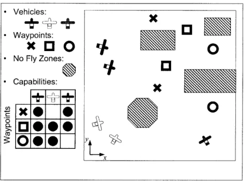
Before trajectories can be designed for the UAVs in the fleet, the control architecture solves an allocation problem to determine a sequence of waypoints for each vehicle to visit. An example of a fleet coordination scenario is shown in Fig. 1-1. In the simplest form of the waypoint allocation problem, every waypoint must be visited while avoiding obstacles. Additional constraints can be added to this problem to capture different types of waypoints representing sites at which to collect sensor information, high value targets which must be destroyed, or anti-aircraft defenses whose destruction might increase the probability of mission success. Only a subset of the fleet might be capable of visiting each waypoint. Timing constraints can be added to enforce simultaneous, delayed or ordered arrival at waypoints. Designing a detailed overall coordination plan for this mission can be viewed as two coupled decisions. Tasks that achieve the fleet goals must be assigned to each team member, and a path must be

-

Vehicles:

-

Waypoints:

-

No Fly Zones:

-

Capabilities:

xe

₀

1.0000

2000

Y

4

x

Fig. 1-1: Schematic of a typical mission scenario for a UAV fleet with numerous waypoints,

No Fly Zones and capabilities

designed for each team member that achieves their tasks while adhering to spatial constraints, timing constraints, and the dynamic capabilities of the aircraft. The coordination plan is designed to minimize some mission cost, such as completion time or probability of failure.

Consideration of each of the fleet coordination decisions in isolation shows that they are computationally demanding tasks. For even moderately sized problems, the number of combinations of task allocations and waypoint orderings that must be considered for the team formation and task assignment decisions is very large. For the relatively simple coordination problem shown in Fig. 1-1, there are 1296 feasible allocations, and even more possible ordered arrival permutations. Coupling exists between the cost of visiting a particular waypoint and the other waypoints visited by the same vehicle, since the length of the trajectory between them depends on their order. There is also considerable uncertainty in this problem; there

is a probability that a UAV will be destroyed by anti-aircraft defenses during its mission, and the waypoint location information may be uncertain and incomplete. The problem of planning kinematically and dynamically constrained optimal paths, even for one aircraft, is also a very high dimension nonlinear optimization problem due to its size and non-convexity, as described in Section 1.1.1. Furthermore, each UAV trajectory is coupled to all other UAV trajectories by collision avoidance constraints.

As difficult as each of these decisions is in isolation, they are in fact strongly coupled to each other. The optimality of the overall coordination plan can be strongly limited

by incompatible team partitioning or unsuitable task allocation. However, the cost to be

minimized by these decisions is a function of the resulting detailed trajectories. While it is not clear how to partition teams and allocated tasks without full cost information, evaluating the cost of all options would require designing detailed trajectories for an exponential number of possible choices.

1.2.1

Summary Previous Work on the Allocation Problem

This coupling has been handled in one approach [24] by forming a large optimization problem that simultaneously assigns the tasks to vehicles and plans corresponding detailed trajec-tories. This method is computationally intensive, but it is guaranteed to find the globally-optimal solution to the problem and can be used as a benchmark against which approximate techniques can be compared.

Recent research has examined several aspects of the UAV allocation problem. Tabu search has been successfully applied to find near optimal coordination plans for many UAVs and many waypoints which minimize total flight time [16 and the expectation of waypoint visitation value [12]. These approaches include fixed time windows for visiting individual waypoints, but do not include constraints on relative timing of waypoint visits and do not capture the ability of one UAV to decrease risk to another UAV by destroying a threatening

SAM site. A stochastic formulation of allocating weapons to targets has also been

targets, but some targets may be discovered in the future. To maximize the expectation of destroyed target value over the entire engagement, a stochastic integer program is solved to balance the value of firing weapons at the detected targets against the value of holding weapons to fire at undetected targets. This formulation does not involve timing constraints, and each weapon may be fired against only one target.

Recent research that has focused on the structure of UAV coordination systems gives special attention to the Low Cost Autonomous Attack System (LOCAAS). Researchers have suggested a hierarchical decomposition of the problem into levels that include team forming, intra-team task allocation, and individual vehicle control [5]. Recent research has proposed methods for decision making at each of these levels [4]. Minimum spanning trees are found to group together the tasks for each team. The intra-team assignment is then performed using an iterative network flow method. At each iteration, this method temporarily assigns all remaining tasks to vehicles, and fixes the assignment that would be performed first in time. This is repeated until all the tasks are assigned. An approach to the allocation problem has also been suggested that involves a network minimum cost flow formulation [31]. The formulations can be solved rapidly, and model the value of searching for additional targets.

There are disadvantages associated with both the iterative and the minimum cost flow formulations. The iterative network formulation has problems with robustness, feasibility and occasional poor performance. These are related to the inclusion of fixed time windows for certain tasks to be performed. The iterative and minimum cost flow approaches cannot incorporate these constraints directly, and incomplete approaches to adding these constraints are used. Furthermore, the minimum cost flow formulation requires penalties for modifying the allocation so that it does not make frequent reassignments as the mission is performed. This formulation permits only one task to be assigned to each vehicle at a time, resulting in suboptimal results. Market-based allocation methods have been considered for the LOCAAS problem [30] and for the general UAV allocation problem [32]. The types of coupling that these problem formulations address is relatively simple; these control systems realize ben-efits through de-conflicting UAV missions and information sharing, and are not capable of

using more subtle cooperation between UAVs such as opening corridors through anti-aircraft defenses.

Approaches to the allocation problem which emphasize timing constraints have also been proposed [21, 18, 28]. In this approach, detailed paths are selected for each of the vehicles in order to guarantee simultaneous arrival at an anti-aircraft defense system, while minimizing exposure to radar along the way. This is performed through the use of coordination func-tions; each vehicle finds its own minimum arrival time as a function of radar exposure, and communicates their coordination function to the rest of the fleet. Each member of the fleet then solves the same optimization problem to determine the arrival time which minimizes radar exposure and allows all members to arrive simultaneously.

Research has also applied rollout algorithms to UAV control problems [34]. These

algorithms are an approach to solving stochastic scheduling problems [2]. Rollout algorithms repeatedly optimize the next scheduling decision to be made. This scheduling decision is selected to minimize the expectation of the sum its cost and the cost-to-go of applying a base scheduling policy from the resulting state to completion. Since the problem is stochastic, some form of simulation is performed to find the expectation of cost, given the first scheduling decision. The UAV control problem is represented in this framework by the aggregation of finite state automata representing aircraft and targets, and a greedy heuristic is used as the base policy. It has been reported [34] that the rollout algorithm is able to learn strategies such as opening attack corridors to decrease attrition.

1.2.2

Outline of Allocation Problem Approach

Chapter 4 of this thesis presents an approach to the combined resource allocation and tra-jectory optimization aspects of the fleet coordination problem. This approach calculates

and communicates the key information that couples the two problems. This algorithm es-timates the cost of various trajectory options using distributed platforms and then solves a centralized assignment problem to minimize the mission completion time. It performs this estimation by using the same straight line path approximation examined in Chapter 2

for evaluating the receding horizon controller's terminal penalty. The allocation problem is solved as a MILP, and can include sophisticated timing constraints such as "Waypoint A must be visited t minutes before Waypoint B". This approach also permits the cost esti-mation step and detailed trajectory planning for this assignment to be distributed between parallel processing platforms for faster solution.

Chapter 5 considers a stochastic MILP formulation of the allocation problem, which maximizes the expectation of the mission's score. This formulation addresses one of the most important forms of coupling in the allocation problem; the coupling between the mission that one UAV performs and the risk that other UAVs experience. Each UAV can reduce the risk for other UAVs by destroying the anti-aircraft defenses that threaten them. While the approach in Ref. [12] assumes a fixed risk for visiting each of the waypoints, the ability to reduce this threat is not addressed directly by any approach in the allocation literature. The formulation presented in Chapter 5 associates not only a score but also a threat with each waypoint. A waypoint's threat captures the probability that an anti-aircraft defense at that waypoint destroys a nearby UAV during its mission. A waypoint poses no threat if the waypoint does not represent an anti-aircraft defense, or if a UAV has already destroyed it. The solution optimizes the use of some vehicles to reduce risk for other vehicles, effectively balancing the score of a mission, if it were executed as planned, against the probability that the mission can be executed as planned.

Chapter 2

Receding Horizon Control Trajectory

Design

2.1

Introduction

This chapters presents an approach to minimum time trajectory optimization for autonomous fixed-wing aircraft performing large scale maneuvers. These trajectories are essentially pla-nar, and are constrained by no-fly zones and the vehicle's maximum speed and turning rate. MILP is used for the optimization, and is well suited to trajectory optimization because it can incorporate logical constraints, such as no-fly zone avoidance, and continuous constraints, such as aircraft dynamics. MILP is applied over a receding planning horizon to reduce the computational effort of the planner and to incorporate feedback. In this approach, MILP is used to plan short trajectories that extend towards the goal, but do not necessarily reach it. The cost function accounts for decisions beyond the planning horizon by estimating the time to reach the goal from the plan's end point. This time is estimated by searching a graph representation of the environment. This approach is shown to avoid entrapment behind ob-stacles, to yield near-optimal performance when comparison with the minimum arrival time found using a fixed horizon controller is possible, to work on a large trajectory optimization problem that is intractable for the fixed horizon controller, and to plan trajectories that can

be followed by vehicles in a hardware testbed.

This chapter will first present a fixed horizon version of the trajectory planner and a receding horizon controller with a simple terminal penalty for comparison. The control architecture of the improved trajectory planner is presented, including the cost map prepa-ration algorithm and the constraints required to evaluate the new terminal penalty. Finally, simulation and hardware testing results are shown.

2.2

Fixed Horizon Minimum Time Controller

A minimum arrival time controller using MILP over a fixed planning horizon was presented

in Ref. [26]. It designs a series of control inputs {u(i) E R2

: i = 0,1, ... , N - 1}, that give

the trajectory {x(i) E 7?2 :i = 1, 2,... , _{N}. Constraints are added to specify that one of} the N trajectory points x(i) = [Xk+i,1 Xk+i,2]T must equal the goal xgoal. The optimization minimizes the time along this trajectory at which the goal is reached, using N binary decision variables bgoai

E

{0,

1} as

N

min

#1(bgoa,

t) = bgoal,iti (2.1)

u(-)i1

subject to

Xk+i,1 - Xgoal,1 < M(1 - bgoal,i)

Xk+i,1 - Xgoal,1 > -M(1 - bgoal,i)

Xk+i,2 - Xgoal,2 < M(1 - bgoal,i)

Xk+i,2 - Xgoal,2 > -M(1 - bgoal,i)

(2.2)

N

S

bgoal,i = 1 (2.3)

where M is a large positive number, and ti is the time at which the trajectory point x(i) is reached. When the binary variable bgoal,i is 0, it relaxes the arrival constraint in Eqn. 2.2. Eqn. 2.3 ensures that the arrival constraint is enforced once.

To include collision avoidance in the optimization, constraints are added to ensure that

none of the N trajectory points penetrate any obstacles. Rectangular obstacles are used in this formulation, and are described by their lower left corner [uiOW Viow]T and upper right corner [Uhigh Vhigh]T. To avoid collisions, the following constraints must be satisfied by each trajectory point

Xk+i,1

ulow

+ M bobst,1

Xk+i,1 > Uhigh - M bobst,2

Xk+i,2 Ulow + M bobst,3

Xk+i,2 Vhigh - M bobst,4 (2.4)

4

Z

bobst,j 3 (2.5)

j=1

The

jth

constraint is relaxed if basstj = 1, and enforced if bassij = 0. Eqn. 2.5 ensures that at least one constraint in Eqn. 2.4 is active for the trajectory point. These constraints are applied to all trajectory points

{x(i)

: i = 1, 2,. .., N}. Note that the obstacle avoidance

con-straints are not applied between the trajectory points for this discrete-time system, so small incursions into obstacles are possible. As a result, the obstacle regions in the optimization must be slightly larger that the real obstacles to allow for this margin.

The trajectory is also constrained by discretized dynamics that model a fixed-wing aircraft as a point of mass m [26]

zi+1,

0 0 1 0 xi+1,1 0 0

zi+

1,2 0 0 0 1 Xi+1,2 0 0 Ui,1

zi+1,1

0 0 0 0

zi+1,

1 0 ui,2

Xi+1,2 _ 0 0 0 0 . _ 1,2 _ 0 1

The model also includes a limited speed and turning rate. The latter is represented by a limit on the magnitude of the turning force u(i) that can be applied

(2.8)

The constraints of Eqns. 2.7 and 2.8 make use of a linear approximation L2(r) of the 2-norm

of a vector r = (ri, r2)

V [Pi P21 E P

:

L2(r) > r1p1 + r2P2, (2.9) where P is a finite set of unit vectors whose directions are distributed from 0' - 3600. The projection of r onto these unit vectors gives the length of the component of r in the direction of each unit vector. When a sufficient number of unit vectors is used in this test, the resulting maximum projection is close to the length of r. The set of unit vectors P is provided to the MILP problem as a parameter.

Note that in this implementation of the problem, there is only an upper bound on the speed. It is feasible for the speed to fall below vmax, allowing tighter turns. However, for the minimum time solution, it is favorable to remain at maximum speed [26].

This formulation finds the minimum arrival time trajectory. Experience has shown that the computational effort required to solve this optimization problem can grow quickly and unevenly with the product of the length of the trajectory to be planned and the number of obstacles to be avoided [29, 26]. However, as discussed in the following sections, a receding horizon approach can be used to design large-scale trajectories.

2.3

Simple Terminal

Cost

Formulation

In order to reduce the computational effort required and incorporate feedback, MILP has been applied within a receding horizon framework. To enable a more direct comparison of the effects of the terminal penalty, the following provides a brief outline of the receding horizon approach suggested in Ref. [29]. The MILP trajectory optimization is repeatedly applied over a moving time-window of length N. The result is a series of control inputs {u(i)

e R

2 : i = 0, 1, . .. ,

N

- 1}, that give the trajectory {x(i) E R2 _{: i = 1,2,. .. ,N}. The}

28

first part of this input trajectory, of length Ne < N, is executed before a new trajectory is planned. The cost function of this optimization is the terminal penalty

#

2(x(N)), which finds

the 1-norm of the distance between the trajectory's end point and the goal. The formulation is piecewise-linear and can be included in a MILP using slack variables as

min

4

2(x(N)) = Li(xgoai - x(N)) (2.10)

u(-)

where L1(r) evaluates the 1-norm of r as the sum of the absolute values of the components

of r. Slack variables s, and s, are used in the piecewise linear relationships

LI(r) = su

+

s,

su > U

su > -U

sv > V

sV > -v (2.11)

Obstacle avoidance and dynamics constraints are also added. This formulation is equivalent to the fixed horizon controller when the horizon length is just long enough to reach the goal. However, when the horizon length does not reach the goal, the optimization minimizes the approximate distance between the trajectory's terminal point and the goal.

This choice of terminal penalty can prevent the aircraft from reaching the goal when the approximation does not reflect the length of a flyable path. This occurs if the line connecting x(N) and the goal penetrates obstacles. This problem is especially apparent when the path encounters a concave obstacle, as shown in Fig. 2-1. When the first trajectory segment is designed, the terminal point that minimizes the 1-norm distance to the goal is within the concavity behind the obstacle, so the controller plans a trajectory into the concavity. Because the path out of the concavity would require a temporary increase in the 1-norm distance to the goal, the aircraft becomes trapped behind the obstacle. This is comparable to the entrapment in local minima that is possible using potential field methods.

o

$2 as terminal penalty

g₀a

b o0O ₀₀ >o o oo o oo o0o

Fig. 2-1: Trajectory Planned using 1-Norm as Terminal Penalty. Starting point at left, goal at right. Circles show trajectory points. Receding horizon controller using simple terminal penalty

#

2 and N = 12 becomes entrapped and fails to reach the goal.

2.4

Improved Receding Horizon Control Strategy

This section presents a novel method for approximating the time-to-go along a path to the goal which avoids obstacles in order to avoid entrapment. This terminal penalty is implemented in a MILP program, using only linear and binary variables.

2.4.1

Control Architecture

The control strategy is comprised of a cost estimation phase and a trajectory design phase. The cost estimation phase computes a compact "cost map" of the approximate minimum distance to go from a limited set of points to the goal. The cost estimation phase is per-formed once for a given obstacle field and position of the goal, and would be repeated if the environment changes.

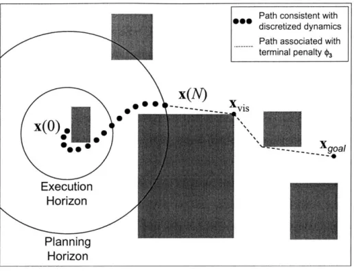
Path consistent with discretized dynamics Path associated with terminal penalty $3

x(O).fl

-x(N) *..*M XXo

0~'

%A

_goal

Execution

Horizon

Planning

Horizon

Fig. 2-2: Resolution Levels of the Planning Algorithm

of the receding horizon optimization. This division of computation between the cost esti-mation and trajectory design phases enables the trajectory optimization to use only linear relationships. This approach avoids the difficulties associated with nonlinear programming, such as choosing a suitable initial guess for the optimization.

An example of a result that would be expected from the trajectory design phase is shown schematically in Fig. 2-2. In this phase, a trajectory consistent with the discretized aircraft dynamics is designed from x(O) over a fine resolution planning horizon of N steps. The trajectory is optimized using MILP to minimize the terminal penalty. This cost estimates the distance to the goal from this point as the distance from x(N) to a visible point xvi,,

whose cost-to-go was estimated in the previous phase, plus the cost-to-go estimate c'is for

xvis. As described in Section 2.4.2, cvis is estimated using a coarser model of the aircraft dynamics that can be evaluated very quickly. Only the first Ne steps are executed before a

new plan is formed starting from the state reached the end of the execution horizon.

The use of two sets of path constraints with different levels of resolution exploits the trajectory planning problem's structure. On a long time-scale, a successful controller need only decide which combination of obstacle gaps to pass through in order to take the shortest dynamically feasible path. However, on a short time-scale, a successful controller must plan the dynamically feasible time-optimal route around the nearby obstacles to pass through the chosen gaps. The different resolution levels of the receding horizon controller described above allow it to make decisions on these two levels, without performing additional computation to "over plan" the trajectory segment to an unnecessary level of detail.

The cost estimation is performed in MATLAB. It produces a data file containing the cost map in the AMPL [9] language, and an AMPL model file specifies the form of the cost function and constraints. The CPLEX [10] optimization program is used to solve the MILP problem and outputs the resulting input and position trajectory. MATLAB is used to simulate the execution of this trajectory up to x(Ne), which leads to a new trajectory optimization problem with an updated starting point.

2.4.2

Computation of Cost Map

The shortest path around a set of polygonal obstacles to a goal, without regard for dynamics, is a series of joined line segments that connect the starting point, possibly obstacle vertices, and the goal. To find this path, a visibility graph can be formed whose nodes represent these points. Edges are added between pairs of nodes if the points they represent can be connected by a line that does not penetrate any obstacles. The visibility graph is searched using Dijkstra's Single Source Shortest Path Algorithm [6], starting at the goal, to find the shortest path from the each node of the graph to the goal, and the corresponding distances.

Dijkstra's Algorithm takes advantage of the fact that if the shortest path from xi to the goal passes through xj, then the portion of this path from xj to the goal is also xj's shortest path. The algorithm maintains two sets of nodes:

K,

whose path to the goal has been fixed, and K, whose path to the goal could still be improved.

K

is initially empty, and

K

initially

algorithm (c, s)

= DIJKSTRA(Xgoai, Xobst, x(O), d)

Place xgoal, all obstacle vertices, and x(O) in

N;

ci := 0,

si

:=

1;

\\

Node 1 is goal

Set all other costs in c to oo;

while

K

#

0

do

Choose the node xj in

A

with minimum c; Move node xj from K to M;

RELAX(jK, C, s, d);

end while

procedure RELAX(j,KV, C, s, d)

for all

nodes xi

E

K

that are connected to xj

do

if

dij

+ cj <

ci

then

ci =dij + cj; \\ Shorten by going through

j

si :=j;

end if

end for

Algorithm 1: Dijkstra's Algorithm. This algorithm provides the basis for Alg. 2

contains all obstacle vertices, the start node, and the goal node. Since optimal trajectories tend to head towards obstacle vertices, these points are a good choice of points at which to find the cost-to-go. Additional points can be added to K.

At each iteration, the algorithm chooses a point of known cost xj to move from

K

to

K,

effectively fixing its path to the goal. In the procedure RELAX, all of the nodes xi that are both connected to xj and in

K

are then examined. If the current route from xi to the goal is longer than the route from xi through xj to the goal, then xi's current minimum distance

ci is updated to this lower value, and

j

is recorded as si, the successor of node i on the path to the goal.

After the distances are updated for all the connected nodes, the minimum of the distance values corresponding to nodes in V is now known with certainty. The node with this

minimum distance is moved to

K.

This process continues until the shortest path from all

nodes to the goal has been found.

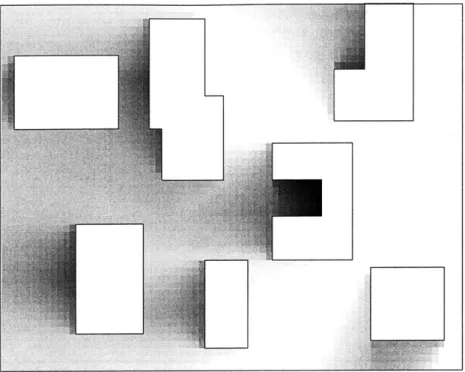
In order to illustrate how the resulting cost map accounts for obstacles, their contribution to the cost is isolated in Fig. 2-3. To produce this graph, cost values were found over a fine

Fig. 2-3: Effect of Obstacles on Cost Values. Difference between actual cost at various

points in an obstacle field and cost in same region with no obstacles, larger differences shown with darker shading. This shows the effects of obstacles on cost values. Goal is at center right.

grid of points in two fields of equal size, one with obstacles, and one without1. The cost values found in the obstacle-free field were subtracted from the cost values found in the obstacle field to remove the contribution of straight line distance to costs. Areas of larger difference are shown in Fig. 2-3 by darker shading. Note that the cost is increasing into the concave obstacle. This increase is crucial to avoiding the entrapment shown in Fig. 2-1.

The major computational activities in the cost estimation phase are determining whether lines intersect with obstacles, and searching through the visibility graph for shortest paths. Computationally efficient ways of doing each are readily available [6], and the entire cost estimation portion of the computation can be performed in a fraction of the time required to form one plan.

'Cost values need not be found over such a fine grid to plan trajectories successfully. Since optimal large-scale trajectories tend to connect the starting point, obstacle vertices, and the goal, costs need only be found at these points. Many extra grid points are added here to more clearly demonstrate the trend in cost values.

2.4.3

Modified MILP Problem

The results of the cost estimation phase are provided to the trajectory design phase as pairs of a position where the approximate cost-to-go is known and the cost at that point (x cSj). This new formulation includes a significantly different terminal cost that is a function of x(N), and (xvis, cis), a pair from the cost estimation phase. The optimization seeks to minimize the distance that must be covered from x(N) to reach the goal by choosing x(N) and the pair (xvi, cviS) that minimize the distance from x(N) to xvi, plus the estimated

distance cvr to fly from xvis to xgoal.

min <3(x(N)) = L2(xvis - x(N)) + c.iS (2.12)

u(

A key element in the algorithm is that the optimization is not free to choose x(N) and xvis independently. Instead, xvi, is constrained to be visible from x(N). Note that visibility constraints are, in general, nonlinear because they involve checking whether every point along a line is outside of all obstacles. Because these nonlinear constraints cannot be included in a MILP problem, they are approximated by constraining a discrete set of interpolating points between x(N) and xvi, to lie outside of all obstacles. These interpolating points are a portion r of the distance along the line-of-sight between x(N) and xvis

V r

C

T : [x(N) + T - (xvis - x(N))] V (2.13) where T C [0, 1] is a discrete set of interpolation distances and XbeSt is the obstacle space.

The visibility constraint ensures that the length of the line between x(N) and xvi, is a good estimate of the length of a path between them which avoids obstacles. The interpolating points are constrained to lie outside obstacles in the same way that the trajectory points are constrained to lie outside obstacles in the previous formulations (see Eqns. 2.4 and 2.5), so it is possible that portions of the line-of-sight between interpolating points penetrate obstacles. However, the number of interpolating points can be chosen as a function of the distance to the goal and the narrowest obstacle dimension to guarantee that the line-of-sight will only be

able to "cut corners" of the obstacles. In this case, the extra distance required to fly around the corner is small, and the accuracy of the terminal penalty is not seriously affected.

The values of the position xvis and cost cvis are evaluated using the binary variables bcost

and the n points on the cost map as

n xvis =

bcostjxcostj

(2.14)

j=1 n C =is = bcost~jCj (2.15) j=1 n

Sbcostj=

1

(2.16)

j=1

Obstacle avoidance constraints (Eqns. 2.4 and 2.5) are enforced without modification at

{x(i) : i = 1,2,... ,

N}.

_{The dynamics model (Eqn. 2.6), the velocity limit (Eqn. 2.7),}

and the control force limit (Eqn. 2.8) are also enforced in this formulation. This provides a completely linear receding horizon formulation of the trajectory design problem.

2.5

Results

The following examples demonstrate that the new receding horizon control strategy pro-vides trajectories that are close to time-optimal and avoid entrapment, while maintaining computational tractability.

2.5.1

Avoidance of Entrapment

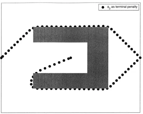
In order to test the performance of the improved cost penalty around concave obstacles, the improved terminal penalty <0₃ was applied to the obstacle field shown in Fig 2-1, and the resulting trajectories are shown in Fig. 2-4. The new cost function captures the difference between the distance to the goal and the length of a path to the goal that avoids obstacles, allowing the receding horizon controller to plan trajectories that reach the goal.

g $3 as terminal penalty

,* 0 _0e

0 0 ,

0 0

0 0'

Fig. 2-4: Trajectories designed using receding horizon controller with

#3

terminal penalty

avoid entrapment. Trajectories start at left and at center, goal is at right. Circles show trajectory points. N = 12.

2.5.2

Performance

The computational effort required by the receding horizon control strategy is significantly less than that of the fixed horizon controller because its planning horizon is much shorter. However, for the same reason, global optimality is not guaranteed. To examine this

trade-off, a set of random obstacle fields was created, and a trajectory to the goal was planned

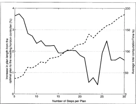
using both the receding and fixed horizon controllers. The receding horizon controller was applied several times to each problem, each time with a longer planning horizon. The results are shown in Fig. 2-5. The extra number of time steps in the receding horizon controller's trajectory is plotted as a percentage of the minimum number of steps found using the fixed horizon controller, averaged over several obstacle fields. The plot shows that, on average, the receding horizon controller is within 3% of the optimum for a planning horizon longer than 7 time steps. The average total computation time for the receding horizon controller is also plotted, showing that the increase in computation time is roughly linear with plan

Fig. 2-5: The Effects of Plan Length. Increase in arrival time from optimal to that found by receding horizon controller is plotted with a solid line. Average total computation time

is plotted with a dashed line.

length.

2.5.3

Computation Savings

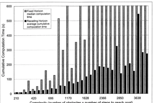
The effects of problem complexity on computation time were also examined by timing the fixed and receding horizon controllers' computation on a 1 GHz PIII computer. The com-plexity of a MILP problem is related to its number of binary variables. For the fixed horizon trajectory designer, the number of binary variables required for obstacle avoidance domi-nates the total number of binary variables as the problem size grows. Four binary variables are required for every obstacle at every time step, so the product of the number of time steps required to reach the goal and the number of obstacles was chosen as a metric of com-plexity. A series of obstacle fields was created with increasing values of this metric, and a trajectory through each obstacle field was planned using both the receding and fixed horizon controllers. Unlike the previous test, the receding horizon controller was applied here with

600 W i I- r ..-it-t u-u-nu L-r 500 --- 1 *Receding Horizon ---- --- --- - - - - - - - -average cumulative computation time E J400 --- -- - - - --- -.0

~-

300 - ---- - -S200- _{1L 0 0 -- --} - -- ---- --- - - - -- -E 0 210 420 686 1170 1628 2366 2850 3638

Complexity (number of obstacles x number of steps to reach goal)

Fig. 2-6: Cumulative Computation Time vs. Complexity

a fixed-length planning horizon. The optimization of each plan was aborted if the optimum was not found in 600 seconds.

The results of this test are shown in Fig. 2-6, which gives the average cumulative com-putation time for the receding horizon controller, and the median comcom-putation time for the fixed horizon controller. The median computation time for the fixed horizon controller was over 600 seconds for all complexity levels over 1628. At several complexity levels for which its median computation time was below 600 seconds, the fixed horizon controller also failed to complete plans. The cumulative time required by the receding horizon controller to design all the trajectory segments to the goal was less than this time limit for every problem. All but the first of its plans can be computed during execution of the previous, so the aircraft can begin moving towards the goal much sooner.

Fig. 2-7: Sample Long Trajectory Designed using Receding Horizon Controller. Executed

trajectory (plan plus velocity disturbance) shown with thick line, planned trajectory seg-ments shown with thin lines.

receding horizon controller. It successfully designed a trajectory that reached the goal in

316 time steps, in a cumulative computation time of 313.2 seconds. This controller took 2.97 seconds on average to design one trajectory segment. The fixed horizon controller

could not solve this problem in 1200 seconds of computation time. A trajectory through the same obstacle field was also planned in the presence of velocity disturbances, causing the followed trajectory to differ significantly from each of the planned trajectory segments.

By designing each trajectory segment from the state that is actually reached, the receding

horizon controller compensates for the disturbance. The executed trajectory and planned trajectory segments are shown in Fig. 2-7.

2.5.4

Hardware Testing Results

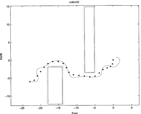
The receding horizon controller was also used to plan a trajectory for a hardware testbed system. This system was made up of radio-controlled trucks equipped with GPS for state estimation [20]. This trajectory was provided as a reference to a controller on board each truck, and is plotted along with the trajectory that the vehicles actually followed in Fig.

2-8. The truck successfully avoided the obstacles and reached its goal. Due mainly to a time

delay between state estimation and steering actuation, the reference trajectory is not followed exactly. However, the reference's selected minimum radius of curvature is clearly larger than the vehicle's turning radius, indicating that the model of the vehicle dynamics restricts the formulation to planning maneuvers that are compatible with the vehicle's turning radius.

video02 15 I 10- 5- 0--5-4 1 |1 -10--25 -20 -15 -10 -5 0 5 East

Fig. 2-8: Planned and Executed Trajectories for Single Vehicle. Time steps making up the planned trajectory are shown with circles. Positions recorded during execution are shown with solid line. Vehicle starts at right and finishes at left. Note that due to the discretization of obstacle avoidance, the obstacles were increased to guarantee that the original obstacles were not penetrated between time steps.

Next, trajectories were planned in a combined optimization for two trucks starting at opposite ends of an obstacle field. Inter-vehicle collision avoidance was enforced similarly to obstacle avoidance, but with a prohibited square of size 5m around each vehicle's time-varying position, instead of the fixed obstacle rectangle. The executed trajectories are plotted together with the planning trajectories in Fig. 2-9. This indicates that inter-vehicle colli-sion avoidance can be enforced by a receding horizon planner which simultaneously plans trajectories for both vehicles.

2.5.5

Planning with Incomplete Information

The examples presented so far have assumed that the position of all obstacles was known at the beginning of the trajectory design and execution process. To examine the effects of

0 Z 0-N -10-II i 1 i i1 -25 -20 -15 -10 -5 0 5 East

Fig. 2-9: Planned and Executed Trajectories for Two Vehicles. Time steps making up the

planned trajectory are shown with circles. Positions recorded during execution are shown with solid line. Grey vehicle starts at left, black vehicle starts at right and vehicles exchange sides. Note inter-vehicle collision avoidance at center.

imperfect obstacle position information, simulations were performed that model a vehicle which begins with no obstacle information, but detects obstacles when they come within some range of it. It is assumed that the obstacles do not move. The detection range was chosen to be longer than the distance that the vehicle could cover over the execution horizon, to avoid collisions.

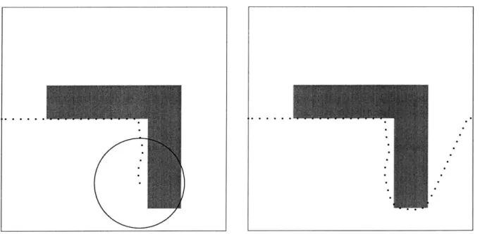
A simulation was performed in a relatively simple environment, and the vehicle's position

and obstacle information is shown in Figs. 2-10 - 2-13. In this simulation, the vehicle takes

an inefficient route, but still reaches the goal because its cost map is updated when new information is received. This update is performed rapidly, requiring a fraction of the time required to optimize one trajectory segment.

The long trajectory planning problem of Fig. 2-7 was also attempted with imperfect obstacle information, and the resulting trajectory to the goal is shown in Fig. 2-14. In this