Convergence in international output

Digitized

by

the

Internet

Archive

in

2011

with

funding

from

Boston

Library

Consortium

Member

Libraries

working paper

department

of

economics

Convergence

in

International Output

massachusetts

institute

of

technology

50 memorial

drive

Convergence

in

International

Output

Andrew

B.

Bernard

Steven

N.

Durlauf

Convergence

in

International

Output

1

Andrew

B.

Bernard

Department

of

Economics

M.I.T.

Cambridge,

MA

02139

Steven

N.

Durlauf

Department

of

Economics

Stanford

University Stanford,

CA

94305

May,

1993

*We

thank Suzanne Cooper,

Chad

Jones, and Paul

Romer

for useful discussions.

The

authors

alsothankparticipants at the

NBER

Summer

Workshop

on

Common

ElementsinTrends and Fluc-tuations,seminarsat Cambridge,Oxford, and LSE, and3

anonymous

referees forhelpfulcomments.

The

Center for Economic Policy Research provided financial support. Bernard gratefully

Summary

This

paper

proposes

and

tests

new

definitions ofconvergence

and

common

trends forper

capita output.

We

define convergence for a

group

ofcountries to

mean

that each country

has identical long-run trends, either stochastic or deterministic, while

common

trends allow

forproportionality ofthe stochastic elements.

These

definitions lead naturally tothe use of

cointegration techniques in testing. Using century-long time series for 15

OECD

economies,

we

reject convergence but find substantial evidence for

common

trends. Smaller samples of

European

countries also reject convergence but are driven

by a

lower

number

of

common

stochastic trends.

1

Introduction

One

of the

most

striking features of the neoclassical

growth model

is its implication for

cross-country convergence. In standard formulations ofthe infinite-horizon optimal

growth

problem, various turnpike theorems

show

that steady-state per capita output is

indepen-dent ofinitial output levels. Further, differences in

microeconomic

parameters will

gener-ate stationary differences in per capita output

and

will not imply different

growth

rates.

Consequently,

when

one

observes differences in per capita output

growth

across countries,

one

must

either

assume

that these countries

have

dramatically different

microeconomic

characteristics, such as different production functions or discount rates, or regard these

discrepancies as transitory.

Launched

primarily

by

the theoretical

work

of

Romer

(1986)

and Lucas

(1988),

much

attention has

been

focused

on

the predictions of

dynamic

equilibrium

models

for long-term

behavior

when

various

Arrow-Debreu

assumptions are relaxed.

Lucas

and

Romer

have

shown

that divergence in long-term

growth

can be generated

by

social increasing returns to

scale associated with

both

physical

and

human

capital.

An

empirical literature exploring

convergence has developed in parallel to the

new

growth

theory.

Prominent

among

these

contributions is the

work

of

Baumol

(1986),

DeLong

(1988),

Barro

(1991)

and

Mankiw,

Romer,

and

Weil (1992). This research has interpreted afinding ofanegative cross-section

correlation

between

initial

income

and growth

rates as evidence in favor ofconvergence.

The

useof cross-section results toinfer the long-run behavior of nationaloutput ignores

valuable information in the time series themselves,

which

can lead to a spurious finding of

convergence. First, it is possibleforaset of countries

which

are diverging to exhibit thesort

ofnegativecorrelation described

by

Baumol

et al. solong asthemarginalproduct of capital

is diminishing.

As shown

by Bernard

and

Durlauf (1992),

a

diminishing marginal product

ofcapital

means

that short-run transitional

dynamics and

long-run, steady-state behavior

will be

mixed up

in cross-section regressions. Second, the cross-section procedures

work

with the null hypothesis that

no

countries are converging

and

the alternative hypothesis

that all countries are,

which

leaves out a host ofintermediate cases.

In this paper

we

propose a

new

definition

and

set oftests ofthe convergence hypothesis.

Our

research differs

from most

previous empirical

work

in that

we

test convergence in an

explicitly stochastic

framework.

If long-run technological progress contains a stochastic

trend, or unit root, then convergenceimplies that the

permanent components

in output are

the

same

across countries.

The

theoryofcointegration provides a natural settingfortesting

cross-country relationships in

permanent

output

movements.

Our

analysis,

which

examines

annuallogreal output per capitafor 15

OECD

economies

from

1900 to 1987, leads to

two

basic conclusions

about

international output fluctuations.1

First,

we

find very little evidence of convergence across the economies. Per capita output

deviations

do

not

appear

to disappear systematically over time. Second,

we

find that there

is strong evidence of

common

stochastic elements in long-run

economic

fluctuations across

countries.

As

a result,

economic growth

cannot be explained exclusively

by

idiosyncratic,

country-specific factors.

A

relatively small set of

common

long-run factors interacts with

individual country characteristics todetermine

growth

rates.

Our

work

is related to studies

by

Campbell and

Mankiw

(1989), Cogley (1990),

and

Quah

(1990)

who

have

explored patterns of persistence in international output. Using

quarterly post-1957 data,

Campbell and

Mankiw

demonstrate

that 7

OECD

economies

exhibit

both

persistence

and

divergence in output. Cogley,

examining

9

OECD

economies

using a similar data set to the

one

here, concludes that persistence is substantial for

many

countries; yetat the

same

time he arguesthat

common

factors generatingpersistence imply

that "long run

dynamics

prevent output levels

from

diverging

by

too

much."

Quah

finds

a lack of convergence for a

wide

range of countries

on

the basis of post-1950 data.

Our

analysis differs

from

this previous

work

in three respects. First,

we

directly formulate the

relationship

between

cointegration,

common

factors,

and

convergence,

which

permits one

to distinguish

between

common

sources of

growth and

convergence. Second,

we

attempt

to

determine

whether

there are subgroups ofconverging countries

and

thereby

move

beyond

the all or nothing

approach

of previous authors. Third,

we

employ

different econometric techniques

and

data sets

which

seem

especially appropriate for the analysis of long-term

'The countries are: Australia, Austria, Belgium, Canada, Denmark, Finland, France, Germany, Italy,

growth

behavior.

The

spirit ofour analysis has

much

in

common

with

work

by Pesaran, Pierse

and

Lee (1993)

and

Lee, Pesaran,

and

Pierse (1992),

who

study multisector output persistence for

the

US

and

UK

respectively.

These

papers derive

methods

to

measure

the long run effects

ofa shock originating in one sector

on

all sectors in the

economy.

While

the focus of that

research has

been

on measuring

persistence rather than convergence, a useful extension

of the current

paper would

be the application of the multivariate persistence

measures

to

international

data

to

both

provide additional tests of convergence as well as to provide a

The

plan of the

paper

is as follows: Section 2 provides definitions of convergence

and

common

trends using a cointegration

framework.

Section 3 outlines the test statistics

we

use. Section 4 describes the data. Section 5 contains the empirical results.

The

evidence

from

the cross-country analysis argues against the notion of convergence for the whole

sample. Alternatively there

do appear

to be groups of countries with

common

stochastic elements.

2

Convergence

in

stochastic

environments

The

organizing principles ofourempirical

work

come

from employing

stochasticdefinitions for

both

long-term

economic

fluctuations

and

convergence.

These

definitions rely

on

the

notions of unit roots

and

cointegration in time series.

We

model

the individual output series as satisfying

Equation

2.1:

a(L)Y

i<t

=

m

4

£i,i (2.1)

where

a(L) has

one

root

on

the unit circle

and

£_1){ is a

mean

zero stationary process.

This formulation allows for

both

linear deterministic

and

stochastic trends in output.

The

interactions of

both

types of trends across countriescanbe formalizedintogeneraldefinitions

ofconvergence

and

common

trends.

Definition

2.1.

Convergence

in

per

capita output

Log

per capita outputs in countries 1,. ..,p converge if

1. Yi

tt,

•.-lYpj satisfy Equation 2.1,

2. /x,

=

fij Vi,j, 3. Yitt,

.

-,Y

Ptt are cointegrated with a cointegrating matrix, /3', such that

0'

=

_{[/„_!,}

-e

_p_i] (2-2)

where I

p-\ is a

p—\

identity matrix

and

ev-\

wop-lxl

vectorofones.

Definition

2.2.

Common

treadsin per capitaoutput

Long-run

logpercapita outputs in countries l,...,p aredetermined by

common

trends if

2.

m

=

fij

V

i,j, 3. yj.t,..

.,

Y

p j are cointegrated.

The

first definition gives us a formal definition ofconvergence. Ifcountries are to attain the

same

long-run

growth

rates withoutput levels separated only

by

astationary difference,

then they

must

satisfy Definition 2.1.

Each

series

must

contain the

same

time trend

and

be

cointegrated with every other series with the cointegrating vector (1,-1).

However,

ifa

group

ofoutput series does not satisfy Definition 2.1, but instead satisfies

the

weaker

Definition 2.2, then output levels will

be

cointegrated but the stochastic trends

for the

group

will not be equal. It will

remain

true that

permanent

shocks will be related

across countries. This is the natural definition to

employ

if

we

are interested in the

pos-sibility that there are a small

number

of stochastic trends affecting output

which

differ in

magnitude

across countries.

The

role oflinear deterministic trends in our analysis is straightforward. If countries'

outputs contain linear trends, then long-run levels

and growth

rates will be equal only if

those trends are identical across all countries.

Thus

both

convergence

and

common

in

any

group

require that all countries have the

same

linear trend. In practice

we

will find that

output for all countries in our

sample

is well

modeled by a

stochastic trend.2

Our

definitionofconvergenceis substantiallydifferent

from

that

employed by

Baumol

et

al.

who

have

defined convergence to

mean

that there is

a

negative cross-section correlation

between

initial

income

and

growth, thereby inferring long-run output behavior

from

cross-section behavior.

Our

analysis studies convergence

by

directly

examining

the time series

properties of variousoutput series,

which

places the convergence hypothesis in

an

explicitly

dynamic and

stochastic environment.

One

potential difficulty with the use of unit root tests to identify convergence is the

presence of a transitional

component

in the aggregate output of various countries.

Time

series tests

assume

that the data are generated

by an

invariant measure, i.e. the

sample

moments

ofthe

data

are interpretable as population

moments

fortheunderlying stochastic

process. Ifthecountriesinour

sample

startat different initial conditions

and

areconverging

to, but are not yet at a steady state output distribution, then the available

data

may

be

generated

by

a transitional law of

motion

rather than

by an

invariant stochastic process.

Consequently, unit root tests

may

erroneouslyaccept a

no

convergence null. Simulations in

Bernard and Durlauf

(1992) suggest that the size distortions are unlikely to be significant. Results are available upon requestfiom the authors.

3

Output

relationships across countries

3.1

Econometric methodology

In order to test for convergence

and

common

trends,

we

employ

multivariate techniques

developed

by

Phillips

and

Ouliaris (1988)

and

Johansen(1988)

Let _j/i

tt denote the log per capita output level ofcountry i

and

Z?y,if the deviation of

output incountry i

from

output in country 1, i.e. j/ijt

-

y,->t.

Y

_t is defined as the

n x

1 vector

ofthe individual output levels,

AY

t as thefirst differenceof

Y

t,

DY

t as the

(n-l)xl

vector

ofoutput deviations, Z?j/,,t,

and

ADY

t the first differences of the deviations.

The

starting point for the empirical

work

is the finding that the individual elements

ofthe per capita output vector are integrated of order one. It is then natural to write a

multivariate

Wold

representation ofoutput as

AY

t

=

n

+

C(L)e

t. _(3.1)

As shown

by

Engle

and Granger

(1987),ifthe

_p

output series arecointegratedin levels with

rcointegrating vectors then

C(l)

is ofrank

p—r

and

thereis

a

vector

ARMA

representation.

A

first test for the

number

oflinearly-independent stochastic trends has

been

developed

by

Phillips

and

Ouliaris (1988)

who

analyze the spectral density matrix at the zero frequency.

A

second test is

due

to

Johansen

(1988, 1989)

who

estimates the rank of the cointegrating matrix.

For a vector ofoutput series, convergence

and

common

trends

impose

different restric-tions

on

the zero frequency of the spectral density matrix of

AY

t,f^y(0)-

Convergence

requires that the persistent parts

be

equal;

common

trends require that thepersistent parts

of individual output series be proportional. In a multivariate

framework,

proportionality

and

equality ofthe persistent parts corresponds to linear dependence,

which

is formalized

as a condition

on

the rank ofthe zero-frequency spectral density matrix.

From

Engle

and

Granger

(1987),ifthe

number

ofdistinct stochastic trends in

Y

t isless

than

n, then

/Ay(0)

isnot offullrank. Ifall

n

countries areconverginginper capitaoutput, then /^dk(0),,,

=

Vt, or equivalently, the rank of

_/ady(0)

is 0.

On

the other hand, if several output series

have

common

persistent parts, the output deviations

from

a

benchmark

country

must

all have zero-valued persistent

components.

Spectral-based procedures devised

by

Phillips

and

Ouliaris permit

a

test for complete convergenceas well as the determination ofthe

number

of

common

trends forthe 15 output

series.

The

tests

make

use of the fact that the spectral density

matrix

offirst differences

stochastic trends in the data

and n

is the

number

ofseries in the sample. This reduction

in rank is captured in the eigenvalues of the zero frequency ofthe spectral density matrix.

If the zero frequency matrix is less than full rank, q

<

n

then the

number

of positive

eigenvalues will also be q

<

n.

The

particular Phillips-Ouliaris test

we

employ

is a

bounds

test that

examines

the smallest

m

=

n

—

q eigenvalues to determineiftheyare close to zero.

We

use

two

critical values for the

bounds

test,

C\

=

0.10^

and

Ci

=

0.05.

These

critical

values assess the averageof the

m

smallest eigenvalues in

comparison

to the average ofall

the eigenvalues.

The

first critical value, Cj, is

m

x

10%

of the average root.

The

second

critical value, C?, corresponds to

5%

ofthe total variance.

For the

Johansen

tests

we

impose

some

additional structure

on

the output series.

We

assume

that afinite-vector autoregressiverepresentation exists

and

rewrite theoutputvector

process as,

£Y

t

=

T(L)&Yt

+

nYt-i+ii

+

et (3.2)

where

and

T,

=

-(A

t+1

+

...-A

k), (t

=!,...,*-!),

ll

=

-(I-A

l

-...-A

k).

II represents the long-run relationship of the individual output series, while

T(L)

traces

out the short-run

impact

of shocks to the system.

We

are interested only in the long-run

relationships,

and

thus all the tests

and

estimates ofcointegrating vectors

come

from

the

matrix, II,

which

can be written as

II

=

a(3' (3.3)

with

q

and

0,

p x

r matrices of rank r

<

p. /? is the matrix of cointegrating vectors, as /3'Yt-k

must

be stationary in

Equation

3.2.

However,

/? is not uniquely determined; a

different choice of

a

satisfying

Equation

3.3 will

produce

a different cointegrating matrix.

Regardless of the normalization chosen, the rank of II is still related to the

number

of

cointegrating vectors. If the rank of II equals p, then Yt is a stationary process. If the

the

rank

of II is

<

r

<

p, there are r cointegrating vectors for the individual series

in

Y

t

and

hence the

group

of time series is being driven

by

p—r

common

shocks. If the

rank ofII equals zero, there are

_p

stochastic trends

and

the long-run output levels are not

related across countries. In particular,

from

Definition 2.1, for the individual output series

to converge there

must be

p—

1 cointegrating vectors of the

form

(1,-1) or

one

common

Two

test statistics proposed by

Johansen

to test the rank of the cointegrating matrix

are derived

from

the eigenvalues of the

MLE

estimate ofII. If

n

is offull rank, p, then it

will have

no

eigenvalues equal to zero. If, however, it isofless

than

full rank, r

<

p, then it

will

have

p—r

zero eigenvalues.

Looking

at the smallest

p-r

eigenvalues the statistics are

p p

trace

=

T ]T

A,;

«

-2ln(Q;r,p)

=

-T

^

/n(l

-

A,) (3.4)

«=r+l i=r+l

and

maximum

eigenvalue

= TA

_r+1 ss

—

2ln(Q;r,

r+

1)

= —

Tln{\

—

A

r+i) (3.5)

The

trace statistic tests the null hypothesis that the rank ofthe cointegrating matrix is r

against the alternative that the rank isp.

The

maximum

eigenvaluestatistic teststhe null

hypothesis that therankis r against the alternative that therankis

r+1.

Critical values for

the asymptotic distributions of

both

statistics are tabulated in

Osterwald-Lenum

(1992).

4

Data

The

data used in the empirical exercise are annual log real

GDP

per capita in 1980

in-ternational dollars.

The

series run

from

1900-1987for 15 industrialized countries with the

GDP

data

drawn

from

Maddison

(1989)

and

the population

data

from

Maddison

(1982).

Population for 1980-1987

comes from IFS

yearbooks.

The

population

data

as published in

Maddison

(1982) are not adjusted to

conform

to

current national borders, while the

GDP

data

are adjusted. Failure to account for border

changes canlead to large

one

time

income

per capita

movements

aspopulation is gained or

lost. For example,

GDP

per capita in the

UK

jumps

in 1920 without

a

correction for the

loss ofthe population of Ireland in that year.

To

avoid these discrete

jumps we

adjust the

population to reflect

modern

borders.3

The

GDP

data set also has a few

minor

problems.

The

year-to-year

movements

during the

two

world wars for

Belgium

and

during

WWI

for

Austriaare constructed

from

GDP

estimates ofneighboring countries.

5

Empirical

results

on

convergence

and

cointegration

In testingforconvergence

and

common

trends,

we

use threeseparate groupingsof countries:

all 15 countries together, the 11

European

countries

and

finally a subset of 6

European

3

This type of gain or loss affects Belgium, Canada, Denmark, Fiance, Italy, Japan, and the

UK

at least once. Ifterritory, and thus population, are lost by country

X

in year Ti, we adjust earlier years by extrapolating backward fromT\ using the year-to-year population changes ofcountry X.

countries

which

exhibit alarge degreeof pairwise cointegration.4 Results

from

the

Phillips-Ouliaris procedures

on

convergence

and

common

trends are in Tables 1

and

2 respectively.

Results using the

Johansen

methods

are in Table 3.

We

initially test for convergence in the 15 country

group

by performing the

Phillips-Ouliaris

bounds

tests

on

the first difference ofoutput deviations,

ADY

t , having subtracted

off the

US

output. If countries converge, then

we

would

expect to find 1 distinct root in

output levels

and no

roots in the deviations

from

a

benchmark

country. If idiosyncratic

trends

dominate

for every country, then

we

would

expect to find

n

distinct roots for

n

countries in the levels. Ifthe

number

ofsignificant roots lies

between

these extremes, this

indicates thepresence of

common

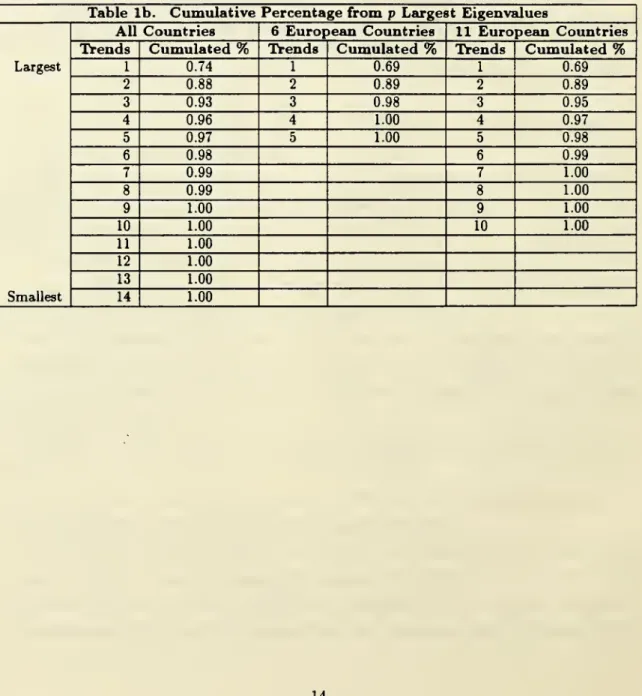
trends in internationaloutput.

As

an

alternative

measure

ofthe

number

of

common

trends,

we

look at the cumulative percentage ofthe

sum

ofthe

roots. Ifthe first

_p

<

n

largest roots contribute

95%

or

more

ofthe

sum,

then

we

conclude

that there are

p

important

common

stochastic trends for the block.5

Table 1 presents the Phillips-Ouliaris

bounds

tests for convergence

and

the cumulative

sums

of the eigenvalues for the groups

mentioned

above.6 Ifthe lower

bound

on

the largest

root is greater

than

the critical level

we

can cannot reject the

no

convergence null.

Ad-ditionally, if the largest root acounts for less than

95%

of the total variance

we

conclude

that there is

more

than one

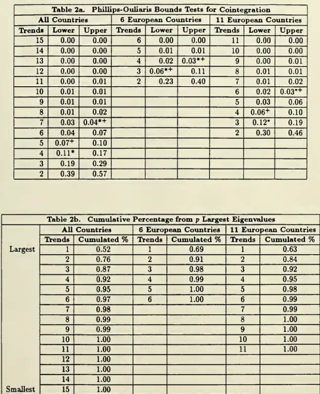
stochastic trend for the group. Table 2 presents

two

different

tests for the

number

of

common

trends in each group. First, ifthe

upper

bound

is less than

the critical value for a given p,

we

can reject the null hypothesis that there are

p

or

more

distinct roots. If the lower

bound

is greater than the

same

critical value then

we

cannot

reject the hypothesis that there are at least

_p

distinct roots.

We

also look for the

number

ofeigenvalues that account for

95%

or

more

of the total variance.

The

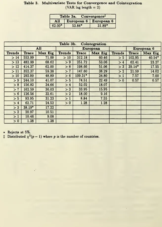
multivariate results

from

the

Johansen

trace

and

maximum

eigenvalue statistics

on

convergence

and

cointegration are presented in Tables

3a

and 3b

for a

VAR

lag length of

2.7

The

two

statistics give different estimates of the cointegrating vectors; the

maximum

eigenvalue test is often not significant for

any

number

of cointegrating vectors. Test results

are presented for null hypotheses

on

number

of

common

trends ranging

from

1 to 15.

The

evidence

on

convergence is quite striking. For all test statistics

and

in all three

samples the convergence hypothesis fails.

The

direct convergence test in Table 1 cannot

reject theno-convergencenullfor

both

critical levelsas thelargest eigenvalue isstatistically

*The 6 European countries are Austria, Belgium, Denmark, France, Italyand the Netherlands. Bernard

(1991) findscointegration in 10of 15 pairs. 5

Cogley (1990) uses asimilar measure.

6

K, thesizeofthe Daniell windowwaschosen to be

T

'6

, or 27for our sample.

7

different

from

zero for all three groupings. Additionally,

both

the trace

and

the

maximum

eigenvalue statistics reject convergence in every

group

in Table 3a.

Having

failed to find evidence for convergence, or a single long-run trend,

we

turn to the test for the

number

of

common

trends.

The

Phillips-Ouliaris statistics for the fifteen

country

sample

and

critical value

C\

(= ^)

reject the null hypothesis that there are 7 or

more

distinct roots

and

cannot reject the null that there are at least 4 distinct roots.

With

the alternative critical value of

5%

of the

sum

of the eigenvalues,Ci,

we

again reject for 7

or

more

distinct rootsbut

now

cannot rejectfor at least 5. This leads us to posit that there

is

a

large

common

stochastic

component

over the sample.

The

six largest roots account for

96.7%

ofthe total, coinciding with the results

from

thetest statistics.

On

the other hand,

the largest root accounts for barely

50%

and

the largest

two

roots for

about

75%

of total

variance,

which

argues against the existence ofjust

a

single

common

factor, as is required

for convergence.

The

Johansen

trace statistic rejects 12 or fewer cointegrating vectors at

the

5%

level

and

13 or fewer at the

10%

level for the entire fifteen country sample. This

implies that there are only

two

or three long-run shocking forces for theentire group.

The

maximum

eigenvalue statistic does not reject for

any

number

of trends.

Taking

all 11 ofthe

European

countries as a group,

we

reject the null hypothesis that

there are 6 or

more

trends

and

cannot reject that there are at least 4 trends with the

C2

statistic

and

that there are at least 3 trends with the

CI

statistic.

The

Johansen

trace

statistic rejects 5 or

more

trends, while the

maximum

eigenvalue test again cannot reject for

any

number

ofcointegrating vectors.

These

results suggest that there are

on

theorder

of 4-5 long-run processes driving output in the

European

countries.

Turning

to the results for the six

European

countries,

we

reject the null that there are

are4 or

more

distinct trends with

both

the

C\ and

Ci

critical values

and

cannot reject the

null that there are at least 3, again with

both

values.

97.8%

of the

sum

comes from

the

three largest eigenvalues. Using

MLE

statistics, the smaller six

European

country

group

rejects2 or

more

trendswith the tracestatistic

and

5or

more

with the

maximum

eigenvalue

test.

6

Conclusions

This

paper

attempts to

answer

empirically the question of

whether

there is convergence in

output per capita across countries.

We

first construct astochastic definition ofconvergence based

on

the theoryof integrated time series.

Time

series forper capita outputofdifferent

countries canfailtoconverge only ifthe persistent parts of thetimeseries aredistinct.

Our

analysis of the relationship

among

long-term output

movements

across countries reveals

little evidence of convergence. Virtually all of our hypothesis tests cannot reject the null

hypothesis of

no

convergence.

On

the other hand,

we

find evidence that there is substantial

cointegration across

OECD

economies.

The number

of integrated processes driving the 15

countries' output series appears to be

on

the order of 3 to 6.

Our

results therefore imply

that there is

some

set of

common

factors which jointly determines international output

growth.

7

References

Barro, R. (1991).

"Economic

Growth

in a Cross Section of Countries." Quarterly Journal of

Economics,

106, 407-443.

Baumol,

W.

(1986). "Productivity

Growth,

Convergence,

and

Welfare:

What

the

Long-Run

Data

Show."

American Economic

Review, 76, 1072-1085.

Bernard, A. (1991). " Empirical Implications ofthe

Convergence

Hypothesis."

Working

Paper, Center for

Economic

Policy Research, Stanford University.

Bernard, A.

and

S. Durlauf. (1992). "Interpreting Tests of the

Convergence

Hypothe-sis."

Working

Paper, Center for

Economic

Policy Research, Stanford University.

Campbell,

J. Y.

and

N. G.

Mankiw.

(1989). "International Evidence

on

the Persistence of

Economic

Fluctuations." Journal of

Monetary Economics,

23, 319-333.

Cogley,T. (1990). "InternationalEvidence

on

The

Sizeofthe

Random

Walk

in Output."

Journal ofPolitical

Economy,

98, 501-518.

DeLong,

J. B. (1988). "Productivity

Growth,

Convergence,

and

Welfare:

Comment."

American

Economic

Review, 78, 1138-1154.

Engle, R. F.

and

C.

W.

J. Granger. (1987). "Cointegration

and

Error-Correction:

Representation, Estimation,

and

Testing." Econometrica,55, 251-276.

Johansen, S. (1988). "Statistical Analysis of Cointegration Vectors." Journal of

Eco-nomic

Dynamics

and

Control, 12, 231-54.

(1991). "Estimation

and

Hypothesis TestingofCointegration Vectorsin

Gaus-sian Vector Autoregressive Models." Econometrica, 59, 1551-1580.

Lee, K.,

M.

Pesaran,

and

R. Pierse. (1992). "Persistence ofShocks

and

their Sources in

aMultisectoral

Model

of

UK

Output Growth."

Economic

Journal, 102,

(March)

342-356.

Lucas, R. E. (1988).

"On

the

Mechanics

of

Economic Development."

Journal of

Mone-tary

Economics,

22, 3-42.

Maddison,

A. (1982).

Phases

of Capitalist Development. Oxford,

Oxford

University Press.

.. (1989).

The

World

Economy

in the 20th Century. Paris,

Development

Centre

ofthe Organisation for

Economic

Co-operation

and Development.

Mankiw,

N.G.,

D.

Romer,

And

D. Weil. (1992).

"A

Contribution to the Empirics of

Economic Growth."

Quarterly Journal of

Economic,

107, 407-438.

Ostewald-Lenum,

M.

(1992). "

A

note with Quantiles ofthe

Asymptotic

Distribution

of the

Maiximum

Likelihood Cointegration

Rank

Test Statistics." Oxford Bulletin of

nomics and

Statistics. 54, 3, 461-472.

Pesaran, M., R. Pierse,

and

K. Lee. (1993). "Persistence, Cointegration,

and

Aggrega-tion:

A

Disaggregated Analysis of the

US

Economy."

Journal ofEconometrics, 56, 57-88.

Phillips, P.C.B.

and

S. Ouliaris. (1988). "Testing for Cointegration Using Principal

Components

Methods."

Journal of

Economic

Dynamics

and

Control, 12, 205-30.

Quah,

D. (1990). "International Patterns of

Growth:

Persistence in

Cross-Country

Disparities."

Working

Paper,

MIT.

Romer,

P. (1986). "Increasing Returns

and

Long

Run

Growth."

Journal of Political

Economy,

94,

1002-1037-Summers,

R.,

and

A. Heston. (1988).

"A

New

Set of International

Comparisons

ofReal

Product and

Price Levels Estimates for 130 Countries, 1950-1985."

Review

of

Income and

Wealth, 34, 1-25.

Table

la. Phillips-Ouliaris

Bounds

Tests for

Convergence

Bounds

Tests**

All

Countries

6

European

Countries

11

European

Countries

Trends

Lower

Upper

Trends

Lower

Upper

Trends

Lower

Upper

<1

1.60+ 3.09

<1

0.68+ 1.32

<1

0.29+ 0.46

Ifthe upper

bound

is below the critical valuefor the largest root, reject null ofno convergence.

Ifthelower

bound

isabovethecriticalvalueforthelargest root,cannotreject nullofnoconvergence.

+

Significant for critical value of0.05.

** _{These statistics are calculated on the vector of first differences of}

_GDPi

_{— GDPk.}

_For

all

countries, the

US

is subtracted off. Forthe 6 European countries, France issubtracted off. For the 11 European countries, France is subtracted off.

Table

lb.

Cumulative

Percentage

from

p Largest Eigenvalues

Largest

Smallest

All

Countries

6

European

Countries

11

European

Countries

Trends

Cumulated

%

Trends

Cumulated

%

Trends

Cumulated

%

1 0.74 1 0.69 1 0.69 2 0.88 2 0.89 2 0.89 3 0.93 3 0.98 3 0.95 4 0.96 4 1.00 4 0.97 5 0.97 5 1.00 5 0.98 6 0.98 6 0.99 7 0.99 7 1.00 8 0.99 8 1.00 9 1.00 9 1.00 10 1.00 10 L 1.00 11 1.00 12 1.00 13 1.00 14 1.00 14

Table

2a. Phillips-Ouliaris

Bounds

Tests for

Cointegration

All

Countries

6

European

Countries

11

European

Countries

Trends

Lower

Upper

Trends

Lower

Upper

Trends

Lower

Upper

15 0.00 0.00 6 0.00 0.00 11 0.00 0.00 14 0.00 0.00 5 0.01 0.01 10 0.00 0.00 13 0.00 0.00 4 0.02 0.03*+ 9 0.00 0.01 12 0.00 0.00 3 0.06*+ 0.11 8 0.01 0.01 11 0.00 0.01 2 0.23 0.40 7 0.01 0.02 10 0.01 0.01 6 0.02 0.03"

+

9 0.01 0.01 5 0.03 0.06 8 0.01 0.02 4 0.06+ 0.10 7 0.03 0.04*+ 3 0.12* 0.19 6 0.04 0.07 2 0.30 0.46 5 0.07+ 0.10 4 0.11* 0.17 3 0.19 0.29 2 0.39 0.57

Table

2b.

Cumulative

Percentage

from

p Largest

Eigenvalues

Largest

Smallest

All

Countries

6

European

Countries

11

European

Countries

Trends

Cumulated

%

Trends

Cumulated

%

Trends

Cumulated

%

1 0.52 1 0.69 1 0.63 2 0.76 2 0.91 2 0.84 3 0.87 3 0.98 3 0.92 4 0.92 4 0.99 4 0.95 5 0.95 5 1.00 5 0.98 6 0.97 6 1.00 6 0.99 7 0.98 7 0.99 8 0.99 8 1.00 9 0.99 9 1.00 10 1.00 10 1.00 11 1.00 11 1.00 12 1.00 13 1.00 14 1.00 15 1.00

Ifthe upper

bound

is below the critical value, reject nullof

P

or

more

distinct roots. Ifthe lower

bound

is above the criticalvalue, cannot reject null ofat least

P

distinct roots.

• Significant atO.lOm/n,

n

is the

number

of countries,

m

isthe

number

of roots

=

0.

+

Significant at

5%

of the

sum

of theroots.

Table

3. Multivariate Tests for

Convergence and

Cointegration

(VAR

lag length

=

2)

Table

3a.

Convergence*

All

European

6

European

6

62.00* 53.84* 31.89*

Table

3b.

Cointegration

All

European

European

6

Trends

Trace

Max

Eig

Trends

Trace

Max

Eig

Trends

Trace

Max

Eig

>

14 553.99 71.00

>

10 312.18 60.46

>5

102.95 40.54*

>13

482.99 68.62

>9

251.72 53.06

>4

62.41 23.27

>

12 414.37 62.00

>8

198.66 51.06

>3

39.14* 17.55

>

11 352.37 59.38

>7

147.60 38.29

>2

21.59 14.02

>

10 292.99 48.89

>6

109.31* _34.80J

>

1 7.57 7.00

>9

244.10 41.07

>5

74.51 22.49

>0

0.57 0.57

>8

156.82 34.66

>4

52.02 18.07

>7

162.59 36.03

>3

33.95 15.95

>6

126.56 32.61

>2

18.00 9.16

>5

93.95 31.23

>

1 8.84 7.55

>4

62.71 24.52

>0

1.28 1.28

>3

38.19* 17.22

>2

20.97 10.51

>

1 10.46 9.08

>0

1.38 1.38 * Rejects at 5%.

t Distributed

x

2(p

—

1) where

p

is the

number

of countries.

7'5

₇₉

16

MIT LIBRARIES DUPL