HAL Id: hal-02001080
https://hal.archives-ouvertes.fr/hal-02001080v2
Submitted on 4 Apr 2019
HAL is a multi-disciplinary open access
archive for the deposit and dissemination of
sci-entific research documents, whether they are
pub-lished or not. The documents may come from
teaching and research institutions in France or
abroad, or from public or private research centers.
L’archive ouverte pluridisciplinaire HAL, est
destinée au dépôt et à la diffusion de documents
scientifiques de niveau recherche, publiés ou non,
émanant des établissements d’enseignement et de
recherche français ou étrangers, des laboratoires
publics ou privés.
Accurate Complex Multiplication in Floating-Point
Arithmetic
Vincent Lefèvre, Jean-Michel Muller
To cite this version:
Vincent Lefèvre, Jean-Michel Muller. Accurate Complex Multiplication in Floating-Point Arithmetic.
ARITH 2019 - 26th IEEE Symposium on Computer Arithmetic, Jun 2019, Kyoto, Japan. pp.1-7.
�hal-02001080v2�
Accurate Complex Multiplication in Floating-Point
Arithmetic
Vincent Lefèvre
*, Jean-Michel Muller
** Univ Lyon, EnsL, UCBL, CNRS, Inria, LIP, F-69342, LYON Cedex 07, France
Abstract—We deal with accurate complex multiplication in binary floating-point arithmetic, with an emphasis on the case where one of the operands is a “double-word” number. We provide an algorithm that returns a complex product with normwise relative error bound close to the best possible one, i.e., the rounding unit 𝑢.
Keywords. Floating-point arithmetic, Complex multiplica-tion, Rounding error analysis.
I. INTRODUCTION AND NOTATION
This paper deals with accurate (from a normwise point of view) complex multiplication in binary floating-point arith-metic, with an emphasis on the case where the real and imaginary parts of one of the operands are “double-word” numbers. This is of interest, for instance, when that operand is a root of one (which is the case in fast Fourier transforms), pre-computed and stored in higher precision than standard floating-point precision. This can also be of interest for computing iterated products of several complex numbers accurately. In the following, we assume a radix-2, precision-𝑝 floating-point arithmetic, with correctly rounded (to nearest) arithmetic operations. We assume that an FMA (Fused Multiply-Add) instruction is available and, to simplify our study, we also assume an unbounded exponent range. This means that the results presented in this paper apply to “real-life” IEEE 754 Floating-Point arithmetic [6] as long as underflows and overflows do not occur.
We will denote 𝑢 = 2−𝑝 the “rounding unit”. For instance in the binary64 format of the IEEE 754 Standard (a.k.a. “double precision”), 𝑢 = 2−53. RN is the round-to-nearest function (with any choice in case of a tie). For instance, when performing the operation 𝑎+𝑏, where 𝑎 and 𝑏 are floating-point numbers, the obtained result is RN(𝑎 + 𝑏), and it satisfies:
|RN(𝑎 + 𝑏) − (𝑎 + 𝑏)| 6 𝑢
1 + 𝑢 · |𝑎 + 𝑏| < 𝑢 · |𝑎 + 𝑏|. When implementing complex operations or functions, if the computed result ^𝑧 has the form ^𝑧𝑅+ 𝑖 · ^𝑧𝐼, where ^𝑧𝑅 and ^𝑧𝐼 are floating-point numbers, and if the exact result is 𝑧 = 𝑧𝑅+ 𝑖 · 𝑧𝐼, one may be interested in minimizing the componentwise relative error max {︂⃒ ⃒ ⃒ ⃒ ^ 𝑧𝑅− 𝑧𝑅 𝑧𝑅 ⃒ ⃒ ⃒ ⃒ ; ⃒ ⃒ ⃒ ⃒ ^ 𝑧𝐼 − 𝑧𝐼 𝑧𝐼 ⃒ ⃒ ⃒ ⃒ }︂ , or the normwise relative error
⃒ ⃒ ⃒ ⃒ ^ 𝑧 − 𝑧 𝑧 ⃒ ⃒ ⃒ ⃒ .
An algorithm that would always return the best possible result (i.e., a real part equal to the floating-point number nearest to the exact real part, and an imaginary part equal to the floating-point number nearest to the exact imaginary part) would have worst case componentwise and normwise relative error 𝑢/(1 + 𝑢) ≈ 𝑢: this is therefore the best error bound achievable by an algorithm that returns the real and imaginary parts of the result in floating point. Our goal here is to obtain small normwise relative errors when computing complex products, i.e., small values of |(^𝑧 − 𝑧)/𝑧|, where 𝑧 is the exact product and ^𝑧 is the computed product.
We will need to represent some variables by double-word numbers. A double-word number (frequently called “double-double” in the literature, because the underlying floating-point format is, in general, the binary64 format) [9], [4] is a pair of floating-point numbers 𝑣ℎand 𝑣ℓthat represents a real number
𝑣 such that
𝑣 = 𝑣ℎ+ 𝑣ℓ,
|𝑣ℓ| 6 12ulp(𝑣)6 𝑢 · |𝑣|.
To compute an approximation ^𝑧𝑅+ 𝑖^𝑧𝐼 to 𝑧𝑅+ 𝑖𝑧𝐼 =
(𝑥𝑅+ 𝑖𝑥𝐼) · (𝑦𝑅+ 𝑖𝑦𝐼), where 𝑥𝑅, 𝑥𝐼, 𝑦𝑅, 𝑦𝐼, ^𝑧𝑅, and ^𝑧𝐼
are floating-point numbers, one may consider the following “naive” formulas:
∙ if no FMA instruction is available {︂
^
𝑧𝑅 = RN(RN(𝑥𝑅𝑦𝑅) − RN(𝑥𝐼𝑦𝐼)), ^
𝑧𝐼 = RN(RN(𝑥𝑅𝑦𝐼) + RN(𝑥𝐼𝑦𝑅)). (1) ∙ if an FMA instruction is available
{︂ ^
𝑧𝑅 = RN(𝑥𝑅𝑦𝑅− RN(𝑥𝐼𝑦𝐼)),
^
𝑧𝐼 = RN(𝑥𝑅𝑦𝐼 + RN(𝑥𝐼𝑦𝑅)). (2)
Formulas (1) and (2), as well as the algorithm we give in this paper (Algorithm 3), can lead to large componentwise relative errors. To obtain small componentwise errors, one needs to use significantly different algorithms, such as an algorithm attributed to Kahan by Higham [5, p. 65], analyzed in [8], or Cornea et al’s algorithm for 𝑎𝑏 + 𝑐𝑑 presented in [2].
Asymptotically optimal bounds on the normwise relative error of formulas (1) and (2) are known: Brent et al. [1] show a bound√5 · 𝑢 for (1), and Jeannerod et al. [7] show a bound 2 · 𝑢 for (2).
We aim at obtaining smaller normwise relative errors, closer to the best possible one, at the cost of more complex algorithms. We consider the product
with
𝑥 = 𝑥𝑅+ 𝑖 · 𝑥𝐼, where 𝑥𝑅 and 𝑥𝐼 are floating-point numbers.
In Section II we deal with the case where the real and imaginary parts 𝜔𝑅 and 𝜔𝐼 of 𝜔 are double-word numbers and the real and imaginary parts of the product are floating-point numbers. The obtained algorithm (Algorithm 3) will then be somehow simplified to consider two cases of interest: the case where the real and imaginary parts of the product are double-word numbers (Section III-A) and the case where 𝜔𝑅
and 𝜔𝐼 are floating-point numbers (Section III-B).
We will need two well-known algorithms of the floating-point literature: Algorithm 2Sum (Algorithm 1 below), that takes two floating-point numbers 𝑎 and 𝑏 as input and returns two floating-point numbers 𝑠 and 𝑡 such that 𝑠 = RN(𝑎 + 𝑏) and 𝑡 = 𝑎 + 𝑏 − 𝑠 (that is, 𝑡 is the error of the floating-point addition of 𝑎 and 𝑏), and Algorithm Fast2Mult (Algorithm 2 below), that requires the availability of an FMA instruction, and takes two floating-point numbers 𝑎 and 𝑏 as input and returns two floating-point numbers 𝜋 and 𝜌 such that 𝜋 = RN(𝑎𝑏) and 𝜌 = 𝑎𝑏 − 𝜋 (that is, 𝜌 is the error of the floating-point multiplication of 𝑎 and 𝑏).
ALGORITHM 1: 2Sum(𝑎, 𝑏). The 2Sum algorithm [12], [11]. 𝑠 ← RN(𝑎 + 𝑏) 𝑎′ ← RN(𝑠 − 𝑏) 𝑏′← RN(𝑠 − 𝑎′) 𝛿𝑎← RN(𝑎 − 𝑎′) 𝛿𝑏← RN(𝑏 − 𝑏′) 𝑡 ← RN(𝛿𝑎+ 𝛿𝑏)
ALGORITHM 2: Fast2Mult(𝑎, 𝑏). The Fast2Mult algo-rithm (see for instance [10], [14], [13]). It requires the availability of a fused multiply-add (FMA) instruction for computing RN(𝑎𝑏 − 𝜋).
𝜋 ← RN(𝑎𝑏) 𝜌 ← RN(𝑎𝑏 − 𝜋)
II. THE MULTIPLICATION ALGORITHM
In this section, we assume that the real and imaginary parts of 𝜔 are double-word numbers, i.e.,
𝜔 = 𝜔𝑅+ 𝑖 · 𝜔𝐼 = (𝜔ℎ𝑅+ 𝜔ℓ𝑅) + 𝑖 · (𝜔𝐼ℎ+ 𝜔ℓ𝐼), where 𝜔𝑅
ℎ, 𝜔ℓ𝑅, 𝜔ℎ𝐼, and 𝜔ℓ𝐼 are floating-point numbers that
satisfy:
∙ |𝜔𝑅ℓ| 6 (1/2)ulp(𝜔𝑅) 6 𝑢 · |𝜔𝑅|; ∙ |𝜔𝐼ℓ| 6 (1/2)ulp(𝜔𝐼) 6 𝑢 · |𝜔𝐼|.
For performing the complex multiplication 𝜔 · 𝑥, we intro-duce Algorithm 3 below. The real part (lines 1 to 9) and the imaginary part (lines 10 to 18) can obviously be computed
in parallel, and within these parts, additional parallelism is possible. For instance lines 3 and 5 can run in parallel with line 1, and line 7 can run in parallel with line 6. This parallelism is easily exploited by recent compilers. This explains the good performance we obtain (see Section IV). Roughly speaking, Algorithm 3 computes the real part 𝑧𝑅 of the result by computing the difference 𝑣𝑅ℎ of the high-order parts of the products 𝜔𝑅ℎ𝑥𝑅 and 𝜔ℎ𝐼𝑥𝐼, and adding the approximated sum 𝛾𝑅
ℓ of all the error terms that could have a significant influence
on the normwise relative error. The imaginary part 𝑧𝐼 of the result is computed in a similar way.
ALGORITHM 3: Accurate complex multiplication 𝜔 · 𝑥, where the real and imaginary parts of 𝜔 = (𝜔ℎ𝑅+ 𝜔𝑅
ℓ ) +
𝑖 · (𝜔𝐼 ℎ+ 𝜔
𝐼
ℓ) are double-word numbers, and the real and
imaginary parts of 𝑥 are floating-point numbers.
1: 𝑡𝑅← RN(𝜔𝐼 ℓ𝑥𝐼) 2: 𝜋𝑅 ℓ ← RN(𝜔ℓ𝑅𝑥𝑅− 𝑡𝑅) 3: (𝑃𝑅 ℎ, 𝑃ℓ𝑅) ← Fast2Mult(𝜔ℎ𝐼, 𝑥𝐼) 4: 𝑟𝑅 ℓ ← RN(𝜋𝑅ℓ − 𝑃ℓ𝑅) 5: (𝑄𝑅 ℎ, 𝑄𝑅ℓ) ← Fast2Mult(𝜔ℎ𝑅, 𝑥𝑅) 6: 𝑠𝑅ℓ ← RN(𝑄𝑅 ℓ + 𝑟 𝑅 ℓ) 7: (𝑣ℎ𝑅, 𝑣𝑅ℓ) ← 2Sum(𝑄𝑅ℎ, −𝑃ℎ𝑅) 8: 𝛾ℓ𝑅← RN(𝑣𝑅 ℓ + 𝑠 𝑅 ℓ) 9: return 𝑧𝑅= RN(𝑣𝑅ℎ + 𝛾 𝑅 ℓ ) (real part) 10: 𝑡𝐼 ← RN(𝜔𝐼 ℓ𝑥 𝑅) 11: 𝜋𝐼ℓ ← RN(𝜔ℓ𝑅𝑥𝐼+ 𝑡𝐼) 12: (𝑃ℎ𝐼, 𝑃ℓ𝐼) ← Fast2Mult(𝜔ℎ𝐼, 𝑥𝑅) 13: 𝑟𝐼ℓ ← RN(𝜋𝐼ℓ+ 𝑃ℓ𝐼) 14: (𝑄𝐼ℎ, 𝑄𝐼ℓ) ← Fast2Mult(𝜔ℎ𝑅, 𝑥𝐼) 15: 𝑠𝐼 ℓ ← RN(𝑄 𝐼 ℓ+ 𝑟 𝐼 ℓ) 16: (𝑣𝐼 ℎ, 𝑣ℓ𝐼) ← 2Sum(𝑄𝐼ℎ, 𝑃ℎ𝐼) 17: 𝛾𝐼 ℓ ← RN(𝑣𝐼ℓ + 𝑠𝐼ℓ) 18: return 𝑧𝐼 = RN(𝑣𝐼 ℎ+ 𝛾ℓ𝐼) (imaginary part)
Our main result is
Theorem 1. As soon as 𝑝> 4, the normwise relative error 𝜂 of Algorithm 3 satisfies
𝜂 < 𝑢 + 33𝑢2.
The condition “𝑝 > 4” of Theorem 1 always holds in practice. Note that Algorithm 3 can easily be transformed into an algorithm that returns the real and imaginary parts of the product as double-word numbers, in order to reduce the error: it suffices to replace the floating-point additions of lines 9 and 18 by a call to 2Sum (or to the somehow simpler Fast2Sum algorithm, see for instance [13]). We deal with this solution in Section III-A.
Theorem 1 uses the following lemma, that we will prove first.
Lemma 1 (Componentwise absolute error of Algorithm 3). We have
|𝑧𝑅− ℜ(𝑤𝑥)|
6 𝛼𝑛𝑅+ 𝛽𝑁𝑅,
|𝑧𝐼− ℑ(𝑤𝑥)|
with 𝑁𝑅 = |𝜔𝑅𝑥𝑅| + |𝜔𝐼𝑥𝐼|, 𝑛𝑅 = |𝜔𝑅𝑥𝑅− 𝜔𝐼𝑥𝐼|, 𝑁𝐼 = |𝜔𝑅𝑥𝐼| + |𝜔𝐼𝑥𝑅|, 𝑛𝐼 = |𝜔𝑅𝑥𝐼 + 𝜔𝐼𝑥𝑅|, 𝛼 = 𝑢 + 3𝑢2+ 𝑢3, 𝛽 = 15𝑢2+ 38𝑢3+ 39𝑢4+ 22𝑢5+ 7𝑢6+ 𝑢7.
Proof. We will focus on the calculation of the real part of the complex product (i.e., lines 1 to 9 of the algorithm), since the results for the real part hold for the imaginary part through a simple symmetry argument (namely, the imaginary part of (𝑎 + 𝑖𝑏) · (𝑐 + 𝑖𝑑) is equal to the real part of (𝑏 − 𝑖𝑎) · (𝑐 + 𝑖𝑑)). A. Lines 1-2 of Algorithm 3: computation of an approximation 𝜋𝑅 ℓ to(𝜔𝑅ℓ𝑥𝑅− 𝜔𝐼ℓ𝑥𝐼). We have |𝑡𝑅− (𝜔𝐼 ℓ𝑥 𝐼 )| 6 𝑢2· |𝜔𝐼𝑥𝐼|, (4) and |𝑡𝑅| 6 (𝑢 + 𝑢2) · |𝜔𝐼𝑥𝐼|, so that |𝜔𝑅 ℓ 𝑥 𝑅− 𝑡𝑅| 6 𝑢 · |𝜔𝑅𝑥𝑅| + (𝑢 + 𝑢2) · |𝜔𝐼𝑥𝐼| 6 (𝑢 + 𝑢2) · (|𝜔𝑅𝑥𝑅| + |𝜔𝐼𝑥𝐼|) = (𝑢 + 𝑢2) · 𝑁𝑅, a consequence of which is |𝜋𝑅 ℓ − (𝜔𝑅ℓ𝑥𝑅− 𝑡𝑅)| 6 (𝑢2+ 𝑢3) · 𝑁𝑅, (5) and |𝜋𝑅 ℓ | 6 (𝑢 + 2𝑢 2+ 𝑢3) · 𝑁𝑅.
From (4) and (5), we obtain ⃒ ⃒𝜋ℓ𝑅− (𝜔ℓ𝑅𝑥𝑅− 𝜔ℓ𝐼𝑥𝐼) ⃒ ⃒6 𝜖1, (6) with 𝜖1= (2𝑢2+ 𝑢3) · 𝑁𝑅. B. Line 3. We have 𝑃ℎ𝑅+ 𝑃ℓ𝑅= 𝜔ℎ𝐼𝑥𝐼, (7) with |𝑃ℓ𝑅| 6 𝑢 · |𝜔 𝐼 ℎ𝑥 𝐼 | 6 𝑢(1 + 𝑢) · |𝜔𝐼𝑥𝐼|, and |𝑃𝑅 ℎ| 6 (1 + 𝑢) 2· |𝜔𝐼𝑥𝐼|. C. Line 4. From |𝜋𝑅 ℓ − 𝑃ℓ𝑅| 6 (𝑢 + 𝑢2) · |𝜔𝐼𝑥𝐼| + (𝑢 + 2𝑢2+ 𝑢3) · 𝑁𝑅 6 (2𝑢 + 3𝑢2+ 𝑢3) · 𝑁𝑅, we obtain |𝑟𝑅 ℓ − (𝜋 𝑅 ℓ − 𝑃 𝑅 ℓ )| 6 𝜖2, (8) with 𝜖2= (2𝑢2+ 3𝑢3+ 𝑢4) · 𝑁𝑅, and |𝑟𝑅 ℓ| 6 (2𝑢 + 5𝑢 2+ 4𝑢3+ 𝑢4) · 𝑁𝑅, (9)
and, using (6) and (8), ⃒ ⃒𝑟𝑅 ℓ − (𝜔𝑅ℓ𝑥𝑅− 𝜔𝐼ℓ𝑥𝐼− 𝑃ℓ𝑅) ⃒ ⃒ 6 (4𝑢2+ 4𝑢3+ 𝑢4) · 𝑁𝑅. (10) D. Lines 5 and 6. We have 𝑄𝑅ℎ + 𝑄𝑅ℓ = 𝜔ℎ𝑅𝑥𝑅, (11) and |𝑄𝑅 ℓ| 6 𝑢(1 + 𝑢) · |𝜔 𝑅𝑥𝑅|.
From this bound on |𝑄𝑅ℓ| and (9), we obtain ⃒
⃒𝑄𝑅ℓ + 𝑟𝑅ℓ⃒⃒6 (3𝑢 + 6𝑢2+ 4𝑢3+ 𝑢4) · 𝑁𝑅, from which we deduce
⃒ ⃒𝑠𝑅ℓ − (𝑄𝑅 ℓ + 𝑟 𝑅 ℓ) ⃒ ⃒6 𝜖3, (12) with 𝜖3= (3𝑢2+ 6𝑢3+ 4𝑢4+ 𝑢5) · 𝑁𝑅, and ⃒ ⃒𝑠𝑅ℓ⃒ ⃒6 (3𝑢 + 9𝑢 2+ 10𝑢3+ 5𝑢4+ 𝑢5) · 𝑁𝑅. (13) All this gives
(𝑄𝑅 ℎ − 𝑃 𝑅 ℎ + 𝑠 𝑅 ℓ) = (𝑄 𝑅 ℎ − 𝑃 𝑅 ℎ + 𝑄 𝑅 ℓ + 𝑟 𝑅 ℓ) +𝜉3 = (𝑄𝑅 ℎ + 𝑄 𝑅 ℓ − 𝑃 𝑅 ℎ + (𝜋 𝑅 ℓ − 𝑃 𝑅 ℓ )) +𝜉3+ 𝜉2 = (𝜔𝑅 ℎ𝑥 𝑅− 𝜔𝐼 ℎ𝑥 𝐼+ 𝜔𝑅 ℓ𝑥 𝑅− 𝜔𝐼 ℓ𝑥 𝐼) +𝜉3+ 𝜉2+ 𝜉1, with |𝜉3| 6 𝜖3= (3𝑢2+ 6𝑢3+ 4𝑢4+ 𝑢5) · 𝑁𝑅, (from (12)), and |𝜉2| 6 𝜖2= (2𝑢2+ 3𝑢3+ 𝑢4) · 𝑁𝑅, (from (8)), and |𝜉1| 6 𝜖1= (2𝑢2+ 𝑢3) · 𝑁𝑅,
(from (6), (7), and (11)). This implies ⃒ ⃒(𝑄𝑅 ℎ − 𝑃 𝑅 ℎ + 𝑠 𝑅 ℓ) − (𝜔 𝑅𝑥𝑅− 𝜔𝐼𝑥𝐼)⃒ ⃒ 6 (7𝑢2+ 10𝑢3+ 5𝑢4+ 𝑢5) · 𝑁𝑅. (14) E. Lines 7 to 9. We have |𝑄𝑅 ℎ − 𝑃ℎ𝑅| = |𝜔ℎ𝑅𝑥𝑅− 𝜔ℎ𝐼𝑥𝐼− 𝑄𝑅ℓ + 𝑃ℓ𝑅| 6 𝑛𝑅+ (2𝑢 + 𝑢2) · 𝑁𝑅, hence, |𝑣𝑅 ℓ | 6 𝑢 · 𝑛 𝑅+ (2𝑢2+ 𝑢3) · 𝑁𝑅, and |𝑣𝑅 ℎ| 6 (1 + 𝑢) · 𝑛 𝑅+ (2𝑢 + 3𝑢2+ 𝑢3) · 𝑁𝑅. Therefore, using (13), |𝑣𝑅 ℓ + 𝑠 𝑅 ℓ| 6 𝑢 · 𝑛 𝑅+ (3𝑢 + 11𝑢2+ 11𝑢3+ 5𝑢4+ 𝑢5) · 𝑁𝑅, so that ⃒ ⃒𝛾𝑅 ℓ − (𝑣ℓ𝑅+ 𝑠𝑅ℓ) ⃒ ⃒ 6 𝑢2· 𝑛𝑅 +(3𝑢2+ 11𝑢3+ 11𝑢4+ 5𝑢5+ 𝑢6) · 𝑁𝑅, (15)
and ⃒ ⃒𝛾ℓ𝑅⃒⃒6 (𝑢 + 𝑢2) · 𝑛𝑅 +(3𝑢 + 14𝑢2+ 22𝑢3+ 16𝑢4+ 6𝑢5+ 𝑢6) · 𝑁𝑅. This gives ⃒ ⃒𝑣𝑅 ℎ + 𝛾 𝑅 ℓ ⃒ ⃒ 6 (1 + 2𝑢 + 𝑢2) · 𝑛𝑅 +(5𝑢 + 17𝑢2+ 23𝑢3+ 16𝑢4+ 6𝑢5+ 𝑢6) · 𝑁𝑅,
so that the error of the final addition 𝑣ℎ𝑅+ 𝛾ℓ𝑅 is bounded by (𝑢 + 2𝑢2+ 𝑢3) · 𝑛𝑅
+(5𝑢2+ 17𝑢3+ 23𝑢4+ 16𝑢5+ 6𝑢6+ 𝑢7) · 𝑁𝑅. (16)
The bound on the total error (i.e., |𝑧𝑅−ℜ(𝑤𝑥)|) is obtained by adding the bounds (14), (15), and (16), i.e.,
(𝑢 + 3𝑢2+ 𝑢3) · 𝑛𝑅
+(15𝑢2+ 38𝑢3+ 39𝑢4+ 22𝑢5+ 7𝑢6+ 𝑢7) · 𝑁𝑅. (17)
This gives Lemma 1.
Let us now prove Theorem 1.
Proof. Lemma 1 gives a bound on the componentwise abso-lute error of Algorithm 3. However, it does not allow one to infer a useful bound on the componentwise relative error, since |𝑁𝑅/𝑛𝑅| and |𝑁𝐼/𝑛𝐼| can be arbitrarily large. However, the
normwise relative error is always small, as we are going to see.
The square of the normwise relative error 𝜂 is
𝜂2= (𝑧 𝑅− ℜ(𝜔𝑥))2+ (𝑧𝐼− ℑ(𝜔𝑥))2 (ℜ(𝜔𝑥))2+ (ℑ(𝜔𝑥))2 . From (3), we have (𝑧𝑅− ℜ(𝜔𝑥))2+ (𝑧𝐼− ℑ(𝜔𝑥))2 6 𝛼2(︁(︀𝑛𝑅)︀2 +(︀𝑛𝐼)︀2)︁ + 2𝛼𝛽(︀𝑛𝑅𝑁𝑅+ 𝑛𝐼𝑁𝐼)︀ +𝛽2(︁(︀𝑁𝑅)︀2 +(︀𝑁𝐼)︀2)︁ . We also have (ℜ(𝜔𝑥))2+ (ℑ(𝜔𝑥))2=(︀𝑛𝑅)︀2+(︀𝑛𝐼)︀2 =(︀𝜔𝑅𝑥𝑅)︀2+(︀𝜔𝐼𝑥𝐼)︀2+(︀𝜔𝑅𝑥𝐼)︀2+(︀𝜔𝐼𝑥𝑅)︀2. Hence, 𝜂2 6 𝛼2+ 2𝛼𝛽𝑛 𝑅𝑁𝑅+ 𝑛𝐼𝑁𝐼 (𝑛𝑅)2+ (𝑛𝐼)2 +𝛽2(︀𝑁 𝑅)︀2 +(︀𝑁𝐼)︀2 (𝑛𝑅)2+ (𝑛𝐼)2 . (18)
We can notice that 𝑛𝑅𝑁𝑅+ 𝑛𝐼𝑁𝐼 (𝑛𝑅)2+ (𝑛𝐼)2 6 (︀𝑁𝑅)︀2 +(︀𝑁𝐼)︀2 (𝑛𝑅)2+ (𝑛𝐼)2 , and (︀𝑁𝑅)︀2 +(︀𝑁𝐼)︀2 (𝑛𝑅)2+ (𝑛𝐼)2 = 1 + 4 · ⃒ ⃒𝜔𝑅𝑥𝑅𝜔𝐼𝑥𝐼⃒ ⃒ (𝜔𝑅𝑥𝑅)2+ (𝜔𝐼𝑥𝐼)2+ (𝜔𝑅𝑥𝐼)2+ (𝜔𝐼𝑥𝑅)2. (19)
In the denominator of the right-hand part of (19), the sum of the two terms(︀𝜔𝑅𝑥𝑅)︀2
and(︀𝜔𝐼𝑥𝐼)︀2
is larger than or equal to 2 ·⃒⃒𝜔𝑅𝑥𝑅𝜔𝐼𝑥𝐼⃒ ⃒, since (︀𝜔𝑅𝑥𝑅)︀2 +(︀𝜔𝐼𝑥𝐼)︀2 − 2 ·⃒ ⃒𝜔𝑅𝑥𝑅𝜔𝐼𝑥𝐼⃒ ⃒ = (|𝜔𝑅𝑥𝑅| − |𝜔𝐼𝑥𝐼|)2 > 0.
The same holds for the sum of the two terms (︀𝜔𝑅𝑥𝐼)︀2 and (︀𝜔𝐼𝑥𝑅)︀2
. This immediately gives 1 + 4 ·
⃒
⃒𝜔𝑅𝑥𝑅𝜔𝐼𝑥𝐼⃒ ⃒
(𝜔𝑅𝑥𝑅)2+ (𝜔𝐼𝑥𝐼)2+ (𝜔𝑅𝑥𝐼)2+ (𝜔𝐼𝑥𝑅)2 6 2.
Combined with (18), this gives
𝜂26 𝛼2+ 4𝛼𝛽 + 2𝛽2, from which we obtain
𝜂2
6 𝑢2+ 66𝑢3+ 793𝑢4+ 2958𝑢5+ 5937𝑢6
+ 7696𝑢7+ 6982𝑢8+ 4596𝑢9+ 2216𝑢10
+ 772𝑢11+ 186𝑢12+ 28𝑢13+ 2𝑢14.
(20)
This bound can be rewritten
𝜂26(︀𝑢 + 33𝑢2)︀2− (296 − 𝜈) · 𝑢4
with
𝜈 = 2958𝑢 + 5937𝑢2+ 7696𝑢3+ 6982𝑢4+ 4596𝑢5 + 2216𝑢6+ 772𝑢7+ 186𝑢8+ 28𝑢9+ 2𝑢10. One easily checks that for 𝑢6 1/16 (i.e., 𝑝 > 4), 𝜈 < 296 (since it is an increasing function of 𝑢, it suffices to check its value for 𝑢 = 1/16). Theorem 1 immediately follows from that.
III. TWO SPECIAL CASES
A. Obtaining the real and imaginary parts of the product as double-word numbers
As explained above, one may wish to obtain the real and imaginary parts of the product 𝜔 · 𝑥 as double-word numbers, by replacing the floating-point addition 𝑧𝑅 = RN(𝑣𝑅
ℎ + 𝛾ℓ𝑅)
of line 9 of Algorithm 3 by a call to 2Sum(𝑣𝑅
ℎ, 𝛾𝑅ℓ), and by
replacing the floating-point addition 𝑧𝐼 = RN(𝑣𝐼
ℎ+ 𝛾𝐼ℓ) of line
18 by a call to 2Sum(𝑣𝐼
ℎ, 𝛾ℓ𝐼). The resulting componentwise
error bound is obtained by adding (14) and (15), so that the values 𝛼 and 𝛽 of Lemma 1 must be replaced by
𝛼′ = 𝑢2 and
With these new values, the square 𝜂′2 of the normwise error now satisfies 𝜂′2 6 241𝑢4+ 924𝑢5+ 1586𝑢6 + 1608𝑢7+ 1060𝑢8+ 468𝑢9 + 136𝑢10+ 24𝑢11+ 2𝑢12, (21)
so that the normwise relative error becomes less than √241 · 𝑢2+ 𝒪(𝑢3) ≈ 15.53𝑢2+ 𝒪(𝑢3).
That variant is of interest if one wishes to accurately evaluate the product
𝑧1× 𝑧2× · · · × 𝑧𝑛
of 𝑛 complex numbers. One can evaluate that product iter-atively, keeping the real and imaginary parts of the partial product of all already considered terms as double-word num-bers, and just using the unmodified Algorithm 3 (i.e., a simple FP addition and not a 2Sum at lines 9 and 18) for the last multiplication. Still assuming that overflow or underflow do not occur (which may become unlikely if 𝑛 is very large and the 𝑧𝑖are arbitrary numbers), the total relative error is bounded
by
(1 + 𝜂′)𝑛−2· (1 + 𝜂) − 1.
For instance, assuming binary64 arithmetic (𝑢 = 2−53), one can multiply 1000 numbers and still have a normwise relative error bounded by 1.000000000001724𝑢.
B. If𝜔𝐼 and 𝜔𝑅 are floating-point numbers
If 𝜔𝐼 and 𝜔𝑅are floating-point numbers (i.e., if 𝜔ℓ𝐼 = 𝜔𝑅ℓ = 0), Algorithm 3 becomes simpler, and we obtain Algorithm 4 below. Each separate part (computation of the real part, lines 1 to 6, or computation of the imaginary part, lines 7 to 12) in Algorithm 4 is similar to Cornea et al’s algorithm for 𝑎𝑏 + 𝑐𝑑 presented in [2] (with an addition replaced here by a call to 2Sum), and to Algorithm 5.3 in [15] (with an inversion in the order of summation of 𝑃𝑅
ℓ , 𝑄𝑅ℓ, and 𝑣ℓ𝑅for the real part, and
of 𝑃𝐼
ℓ, 𝑄𝐼ℓ, and 𝑣ℓ𝐼 for the imaginary part).
ALGORITHM 4: Accurate complex multiplication 𝜔 · 𝑥, where the real and imaginary parts of 𝜔 and the real and imaginary parts of 𝑥 are FP numbers, derived from Algorithm 3. 1: (𝑃𝑅 ℎ, 𝑃ℓ𝑅) ← Fast2Mult(𝜔𝐼, 𝑥𝐼) 2: (𝑄𝑅 ℎ, 𝑄𝑅ℓ) ← Fast2Mult(𝜔𝑅, 𝑥𝑅) 3: 𝑠𝑅 ℓ ← RN(𝑄𝑅ℓ − 𝑃ℓ𝑅) 4: (𝑣𝑅 ℎ, 𝑣ℓ𝑅) ← 2Sum(𝑄𝑅ℎ, −𝑃ℎ𝑅) 5: 𝛾𝑅 ℓ ← RN(𝑣ℓ𝑅+ 𝑠𝑅ℓ) 6: return 𝑧𝑅= RN(𝑣ℎ𝑅+ 𝛾 𝑅 ℓ) (real part) 7: (𝑃ℎ𝐼, 𝑃ℓ𝐼) ← Fast2Mult(𝜔𝐼, 𝑥𝑅) 8: (𝑄𝐼ℎ, 𝑄𝐼ℓ) ← Fast2Mult(𝜔𝑅, 𝑥𝐼) 9: 𝑠𝐼ℓ ← RN(𝑄𝐼 ℓ+ 𝑃 𝐼 ℓ) 10: (𝑣𝐼ℎ, 𝑣ℓ𝐼) ← 2Sum(𝑄𝐼ℎ, 𝑃ℎ𝐼) 11: 𝛾𝐼ℓ ← RN(𝑣ℓ𝐼+ 𝑠𝐼ℓ)
12: return 𝑧𝐼 = RN(𝑣ℎ𝐼 + 𝛾ℓ𝐼) (imaginary part)
Of course the error bounds given by (20) and Theorem 1 still apply. However, one can redo the calculations taking into account the zero terms, and obtain new error bounds with smaller higher-order terms, more precisely, we find
𝜂2 6 𝑢2+ 38𝑢3+ 299𝑢4+ 782𝑢5+ 1025𝑢6 + 768𝑢7+ 336𝑢8+ 80𝑢9+ 8𝑢10. (22) Therefore 𝜂26(︀𝑢 + 19𝑢2)︀2 − (62 − 𝜈) · 𝑢4 with 𝜈 = 782𝑢 + 1025𝑢2+ 768𝑢3+ 336𝑢4+ 80𝑢5+ 8𝑢6. This gives
Theorem 2. As soon as 𝑝> 4, the normwise relative error 𝜂 of Algorithm 4 satisfies
𝜂 < 𝑢 + 19𝑢2.
IV. IMPLEMENTATION AND EXPERIMENTS
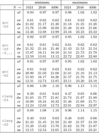
Algorithm 3, implemented in binary64 arithmetic (i.e., 𝑝 = 53 and 𝑢 = 2−53), was compared with other solutions, using a loop over 𝑁 random inputs, itself inside another loop doing 𝐾 iterations. The goal of the external loop is to get precise timings without having to choose a large value of 𝑁 , with input data that would not fit in the cache: we do not want to include memory transfers in the timings. For each test, we chose (𝑁, 𝐾) = (1024, 65536), (2048, 32768) and (4096, 16384).
The other considered solutions were: use of the naive formula (1) in binary64 arithmetic; use of (1) in binary128 (a.k.a. “quad precision”) arithmetic; use of GNU MPFR [3] with precision ranging from 53 to 106 bits either with fused multiplications/subtractions fmma/fmms (thus implementing the formulas, correctly rounded) or with separate additions, subtractions and multiplications.
The tests were run on two machines with a hardware FMA:
∙ an x86_64 machine with Intel Xeon E5-2609 v3 CPUs, under Linux (Debian/unstable), with GCC 8.2.0 and a Clang 8 preversion, using -march=native;
∙ a ppc64le machine with POWER9 CPUs, under Linux (CentOS 7), with GCC 8.2.1, using -mcpu=power9. The following optimization options were used: -O3 and -O2. With GCC, -O3 -fno-tree-slp-vectorize was also used in order to avoid a loss of performance with some vectorized codes. In all the cases, -static was used to avoid the overhead due to function calls to dynamic libraries.
The tests were run on several random data sets, giving a range of timings and a range of ratios. The smallest 10 % values and largest 10 % values have been excluded to take into account inaccuracies in the timings.
We checked that the various timings were globally consis-tent, in particular between the three chosen parameters for (𝑁, 𝐾), and rejected some anomalies manually: for Algo-rithm 3, (𝑁, 𝐾) = (2048, 32768) and (4096, 16384) with
TABLE I
SUMMARY OF THE TIMINGS ON AN X86_64MACHINE(IN SECONDS,FOR 𝑁 𝐾 = 226OPERATIONS). “A3”STANDS FOR“ALGORITHM3” (IN
BINARY64ARITHMETIC), “SW”CORRESPONDS TO THE NAIVE FORMULA (1)IN BINARY64ARITHMETIC, “DW”CORRESPONDS TO(1)IN
BINARY128ARITHMETIC, “CR”ISGNU MPFRWITH FUSED MULTIPLICATIONS/SUBTRACTIONS FMMA/FMMS,AND“NA”ISGNU
MPFRWITH SEPARATE ADDITIONS,SUBTRACTIONS AND MULTIPLICATIONS. minimums maximums 𝑁 → 1024 2048 4096 1024 2048 4096 gcc -O3 a3 0.94 0.97 0.97 0.96 1.02 1.02 sw 0.61 0.62 0.62 0.61 0.62 0.62 dw 21.02 21.17 21.20 21.18 21.25 21.28 cr 15.76 15.99 16.08 21.48 21.63 21.66 na 12.46 12.88 12.99 23.16 23.23 23.22 gcc -O3 -f... a3 0.92 0.97 0.97 0.95 1.02 1.02 sw 0.61 0.61 0.62 0.61 0.62 0.62 dw 21.32 21.44 21.46 21.43 21.53 21.54 cr 15.87 16.11 16.16 21.54 21.73 21.78 na 12.59 13.01 13.12 22.72 22.85 22.80 gcc -O2 a3 0.91 0.97 0.97 0.95 1.02 1.02 sw 0.61 0.62 0.62 0.61 0.62 0.62 dw 20.90 21.03 21.08 21.01 21.10 21.13 cr 15.93 16.17 16.26 21.57 21.70 21.75 na 12.31 12.74 12.85 23.11 23.20 23.18 clang -O3 a3 0.86 1.09 1.10 0.96 1.15 1.15 sw 0.39 0.61 0.63 0.47 0.65 0.66 dw 21.65 21.77 21.81 21.74 21.87 21.88 cr 16.00 16.24 16.32 21.46 21.69 21.71 na 12.24 12.63 12.72 22.91 22.94 22.97 clang -O2 a3 0.88 1.08 1.10 0.96 1.14 1.15 sw 0.40 0.61 0.63 0.48 0.65 0.66 dw 21.33 21.45 21.50 21.49 21.57 21.59 cr 15.38 15.62 15.70 21.62 21.79 21.87 na 12.15 12.54 12.65 23.15 23.21 23.21
Clang gave running times larger than those obtained with GCC, affecting the comparison with GNU MPFR. The timings are given in Table I (x86_64) and Table II (Power9). Note that reading the inputs is included in the timings (thus the ratios will be closer to 1 than one could expect), but these inputs are already in the right format for each implementation.
As a summary from the tables:
∙ Implementation based on the naive formula (1) in
binary64 (inlined code): It is about two times as fast as our implementation of Algorithm 3, but it is significantly less accurate.
∙ Implementation based on the naive formula in bi-nary128, using the __float128 C type (inlined code): On the x86_64 platform, it is from 19 to 25 times as slow as our implementation of Algorithm 3, the reason being that this format is implemented in software. The case of the POWER9 platform is particularly interesting as it has binary128 support in hardware. Here, the implementation is about 2.3 times as slow. This shows that even though
TABLE II
SUMMARY OF THE TIMINGS ON APOWER9MACHINE(IN SECONDS,FOR 𝑁 𝐾 = 226OPERATIONS). “A3” , “SW”, “DW”, “CR”,AND“NA”HAVE THE
SAME MEANING AS INTABLEI.
minimums maximums 𝑁 → 1024 2048 4096 1024 2048 4096 gcc -O3 a3 0.97 0.97 0.97 0.99 0.99 1.00 sw 0.47 0.47 0.51 0.48 0.48 0.52 dw 2.22 2.22 2.22 2.24 2.24 2.24 cr 19.44 19.56 19.62 23.94 24.07 24.06 na 16.41 16.60 16.66 30.07 30.34 30.63 gcc -O3 -f... a3 0.97 0.97 0.97 0.98 0.99 1.00 sw 0.47 0.47 0.51 0.48 0.48 0.52 dw 2.22 2.22 2.22 2.24 2.24 2.24 cr 19.45 19.59 19.61 24.11 24.08 24.07 na 16.42 16.59 16.66 30.06 30.39 30.44 gcc -O2 a3 0.98 0.98 0.98 0.99 1.01 1.01 sw 0.47 0.47 0.51 0.47 0.47 0.51 dw 2.22 2.22 2.22 2.24 2.24 2.24 cr 19.50 19.66 19.68 24.14 24.11 24.05 na 16.36 16.58 16.63 30.29 30.29 30.49
one has hardware support for binary128, there is still interest in algorithms using a mix of binary64 and double-binary64.
∙ Implementation based on GNU MPFR, using
pre-cisions from 53 (corresponding to binary64) to 106 (roughly corresponding to double-binary64). Both codes based on fmma/fmms (thus implementing the formulas, correctly rounded) and based on separate additions, sub-traction and multiplication operations were tested. This is from 11 to 26 times as slow as our implementation of Algorithm 3 on x86_64, and from 17 to 31 times as slow on POWER9.
Algorithm 3 has also been tested on random inputs to search for large normwise relative errors. For binary32, the input values (in ISO C99 / IEEE 754-2008 hexadecimal format) and the corresponding largest error found until now are
𝜔𝑅 = 0x1.b3fdfcp−1 + 0x1.77f658p−26
𝜔𝐼 = 0x1.53c918p−28 + −0x1.ca53e6p−53
𝑥𝑅 = 0x1.2ca11ep−1 𝑥𝐼 = 0x1.9c641ap−18
𝜂 ≃ 0.99999933401292962563 𝑢 and for binary64, we have obtained
𝜔𝑅 = 0x1.d1ef9ea4aa013p−1 + 0x1.ae88ba2a277ep−56 𝜔𝐼 = 0x1.f5c28321df365p−81 + 0x1.c4c3e7b506d06p−135 𝑥𝑅 = 0x1.194f298b4d152p−1 𝑥𝐼 = 0x1.5c1fdca444f7cp−14 𝜂 ≃ 0.99999900913907117123 𝑢.
This corroborates the bound given by Theorem 1. CONCLUSION
We have given algorithms for complex multiplication in floating-point arithmetic, that either return the real and
imag-inary parts of the product as floating-point numbers with a normwise relative error bound close to the best one that one can guarantee, namely 𝑢/(1 + 𝑢), or as double-word numbers. Our implementation is only twice as slow as a significantly less accurate naive implementation. It is much faster than an implementation based on binary128 or multiple-precision software.
ACKNOWLEDGMENT
The authors thank the anonymous reviewers for their very helpful comments. This work has been partly supported by the FastRelax project of the French Agence Nationale de la Recherche (ANR-14-CE25-0018-01).
REFERENCES
[1] R. P. Brent, C. Percival, and P. Zimmermann. Error bounds on complex floating-point multiplication. Mathematics of Computation, 76:1469– 1481, 2007.
[2] M. Cornea, J. Harrison, and P. T. P. Tang. Scientific Computing on Itanium○R-based Systems. Intel Press, Hillsboro, OR, 2002.
[3] L. Fousse, G. Hanrot, V. Lefèvre, P. Pélissier, and P. Zimmermann. MPFR: A multiple-precision binary floating-point library with correct rounding. ACM Transactions on Mathematical Software, 33(2), 2007. 15 pages. Available at https://www.mpfr.org/.
[4] Y. Hida, X. S. Li, and D. H. Bailey. Algorithms for quad-double pre-cision floating-point arithmetic. In 15th IEEE Symposium on Computer Arithmetic (ARITH-15), pages 155–162, June 2001.
[5] N. J. Higham. Accuracy and Stability of Numerical Algorithms. SIAM, Philadelphia, PA, 2nd edition, 2002.
[6] IEEE Computer Society. IEEE Standard for Floating-Point Arithmetic. IEEE Standard 754-2008, August 2008. Available at https://doi.org/10. 1109/IEEESTD.2008.4610935.
[7] C.-P. Jeannerod, P. Kornerup, N. Louvet, and J.-M. Muller. Error bounds on complex floating-point multiplication with an FMA. Mathematics of Computation, 86(304):881–898, 2017.
[8] C.-P. Jeannerod, N. Louvet, and J.-M. Muller. Further analysis of Kahan’s algorithm for the accurate computation of 2 × 2 determinants. Mathematics of Computation, 82(284):2245–2264, 2013.
[9] M. Jolde¸s, J.-M. Muller, and V. Popescu. Tight and rigourous error bounds for basic building blocks of double-word arithmetic. ACM Transactions on Mathematical Software, 44(2), 2017.
[10] W. Kahan. Lecture notes on the status of IEEE-754. Available at https: //people.eecs.berkeley.edu/~wkahan/ieee754status/IEEE754.PDF, 1997. [11] D. E. Knuth. The Art of Computer Programming, volume 2.
Addison-Wesley, Reading, MA, 3rd edition, 1998.
[12] O. Møller. Quasi double-precision in floating-point addition. BIT, 5:37– 50, 1965.
[13] J.-M. Muller, N. Brunie, F. de Dinechin, C.-P. Jeannerod, M. Joldes, V. Lefèvre, G. Melquiond, N. Revol, and S. Torres. Handbook of Floating-Point Arithmetic. Birkhäuser Boston, 2018. ACM G.1.0; G.1.2; G.4; B.2.0; B.2.4; F.2.1., ISBN 978-3-319-76525-9.
[14] Y. Nievergelt. Scalar fused multiply-add instructions produce floating-point matrix arithmetic provably accurate to the penultimate digit. ACM Transactions on Mathematical Software, 29(1):27–48, 2003.
[15] T. Ogita, S. M. Rump, and S. Oishi. Accurate sum and dot product. SIAM Journal on Scientific Computing, 26(6):1955–1988, 2005.