Distinguishing exotic states from scattering states in lattice QCD

Distinguishing Exotic States from Scattering

States in Lattice QCD

by

Dmitry Sigaev

Submitted to the Department of Physics

in partial fulfillment of the requirements for the degree of

Doctor of Philosophy in Physics

at the

MASSACHUSETTS INSTITUTE OF TECHNOLOGY

June 2008

@

Massachusetts Institute of Technology 2008. All rights reserved.

Author ... -...

Department of Physics

May 19, 2008

Certified by ...

John W. Negele

Professor of Physics

Thesis Supervisor

Accepted by ...

Associate Department Head for Education,

T4omas .

reytak

Professo of Physics

ARCHIVES

MASSACHUSETTS INSTITUTE OF TECHNOLOGY OCT 0 9 2008

LIBRARIES

Distinguishing Exotic States from Scattering States in

Lattice QCD

by

Dmitry Sigaev

Submitted to the Department of Physics on May 19, 2008, in partial fulfillment of the

requirements for the degree of Doctor of Philosophy in Physics

Abstract

This work explores the problem of distinguishing potentially interesting new exotic states in QCD from conventional scattering states using lattice QCD, and addresses the specific case of the search for localized resonances in a system of five quarks. We employ a complete basis of local interpolating operators, as well as a number of spatially distributed operators, to search for localized resonances in the system of five quarks. Motivated by initially promising experimental searches for the 8+(1540) pentaquark, we have set out to implement new approaches, both on the theoretical and computational side, to allow for calculations deemed infeasible by other groups searching for pentaquarks on the lattice. We restrict our system of five quarks to the quantum numbers of the E+(1540) pentaquark and get an insight into the structure of its states, calculate their energies and explore their properties. Finally, we use the obtained results to discriminate between scattering and exotic states. The calculation is performed in the quenched approximation with heavy Wilson fermions.

Thesis Supervisor: John W. Negele Title: Professor of Physics

Acknowledgments

I would like to thank Oliver Jahn and John Negele for their continuing help and inspiration. I am grateful to Andrew Pochinsky, Drew Renner and Jonathan Bratt for valuable discussions of this work. And I couldn't have done it without Ilya Sigalov, Gregory Pelts, Cyril Shmatov, and Si-Hui Tan, to whom I would like to say a big thank you.

Contents

1 Introduction

1.1 Background and context ... 1.2 Objectives ...

2 Sources

2.1 Step 1: fixing color structure . . . . 2.2 Step 2: fixing flavor structure . . . 2.3 Step 3: fixing spin/parity . . . . 2.4 Behavior under complex conjugation 2.5 Operators with a definite number of 2.6 Relation between the bases . . . . . 2.7 Relation to other operators . . . . . 2.8 Nucleons and kaons . . . ... 2.9 Scattering states ... 2.10 Operators for scattering states .

upper 21 22 23 27 27 29 30 31 and lower components

3 Spectroscopic analysis

3.1 Equal-time correlation function and the transfer matrix . . . . 3.2 A variation on the traditional variational method . . . .

4 Calculational details 5 Optimizing contractions 5.1 SS block ... ... 39 39 41 45 49 50

5.2 VV block ... ... 52

5.3 SV and VS blocks ... ... 55

6 Lattice results 57 6.1 Nucleons and kaons ... ... 57

6.2 Scattering operators ... ... . 57 6.2.1 Negative parity ... ... . 62 6.2.2 Positive parity ... ... 67 6.3 Local operators ... ... .. 70 6.4 Expansion coefficients ... . ... 73 7 Summary 87

List of Figures

6-1 Sums of nucleon and kaon energies with negative total parity. Different relative momenta have the same line type for the same constituent

hadrons . . . . 59 6-2 Sums of nucleon and kaon energies with positive total parity. Notation

is the same as in Fig. 6-1. ... 60 6-3 Effective masses of eigenvalues for scattering operators with fits and

sums of single-particle energies for a 243 x 64 lattice with mq = m. and negative parity. pl = (0, 0, Po), P2 = (O, po, Po), where po = 2r/L. . . . 63 6-4 Eigenvectors normalized by true norms Ni for a 243 x 64 lattice with

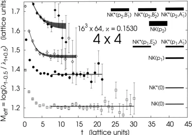
mq = m. and negative parity. ... 64 6-5 Effective masses of eigenvalues for scattering operators with fits and

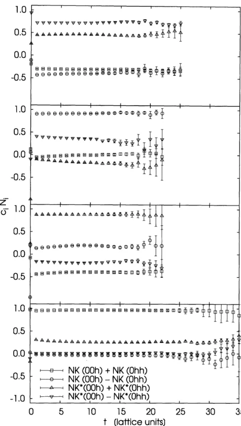
sums of single-particle energies for a 163 x 64 lattice with mq = m. and negative parity. pl = (0, 0,Po), P2 = (O, po, Po), where po = 27/L. . . . 65 6-6 Eigenvectors normalized by true norms Ni for a 163 x 64 lattice with

mq = m. and negative parity. ... 66

6-7 Effective masses of eigenvalues for scattering operators with fits and sums of single-particle energies for a 243 x 64 lattice with mq = ms and

positive parity. pl = (0, 0, po), P2 = (0, po, Po), where po = 27/L. . . . 68

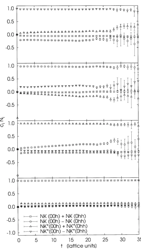
6-8 Eigenvectors normalized by true norms Ni for a 243 x 64 lattice with mq = m. and positive parity ... 69

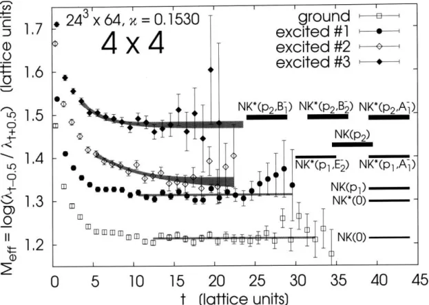
6-9 Effective masses for the lowest three negative parity eigenstates of the 19 x 19 correlation matrix on the 163 x 64 lattice with 'light = 0.1530

and on the 243 x 64 with Klight = 0.1530 and ilight = 0.1558 (top to

bottom). ... 76

6-10 Diagonal matrix elements for three common sources on the 243 x 64 lattice with = 0.1530 ... =light 77 6-11 Diagonalization in two subspaces in the small volume for heavy mass. 78 6-12 Diagonalization in two subspaces in the large volume for heavy mass. 79 6-13 Diagonalization in two subspaces in the large volume for light mass.. 80 6-14 Diagonalization in the space defined by the dominant components. .. 81 6-15 Dependence of energies on to. . ... ... 82 6-16 Dependence of ci(t, to) on t for select to. . ... . 83 6-17 Dependence of cCi(t, to) on to, 243 x 64, , = 0.1530. 7 values of the

coefficients for to = 0..6 are plotted from left to right with the error

band shown in black... 84

6-18 Final expansion coefficients for the lowest three eigenstates. Positive values are shown in dark gray, while negative ones are light gray. . ... 85 6-19 Final expansion coefficients for lowest three eigenstates: alternative

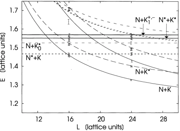
basis . . . .. . . . .. .. 86 7-1 Volume dependence of lowest three states for negative parity. ... 88

7-2 Comparison of energies of lowest three states against the relevant hadron states (refer to Tab. 2.5 for non-zero momentum notation). ... . 89

List of Tables

2.1 Norms squared at infinite quark mass of the two sets of operators used

in this paper. ... 25

2.2 Hadron operators for zero momentum. The superscript ± refers to charge conjugation for the cases with mq = mi. We write 9 = (9_, s+). 32 2.3 Little groups for non-zero momenta and normal vectors to reflection

planes. 0 < a, b, c < 7/alat are assumed to be all different ... . 32 2.4 Decomposition of continuum representations with non-zero momentum

into lattice representations ... 32 2.5 Hadron operators for non-zero momentum. For E representations, sign

alternatives + refer to the two helicity components of the representation. 34 2.6 Representations in 20; induced by product representations of the

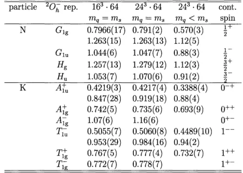
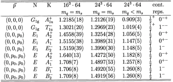
var-ious little groups. ... 35 6.1 Masses of nucleons and kaons at rest. Charge-conjugation labels apply

to the cases with nq = m. only ... 58 6.2 Energies of nucleons and kaons with momentum, where Po = 27/L

denotes the lowest non-zero momentum on the periodic lattice. .... 58 6.3 Sums of nucleon and kaon energies with negative total parity ... 59

Chapter 1

Introduction

Supported by vast experimental evidence, quantum chromodynamics has been es-tablished as the correct theory of strong interactions for decades. Looking at its remarkably simple Lagrangian, one could hope that many aspects of it can be easily developed and understood. However, despite the seeming simplicity and constant effort of the world's best talent, QCD has so far eluded exhaustive mathematical ex-planation. Its significance and difficulty is well illustrated by the fact that one of its fundamental challenges, proving confinement, is among the seven Millennium Prize Problems selected by the scientific advisory board of the Clay Mathematics Institute. We take as a starting line the spectroscopy arm of quantum chromodynamics. One of the things that theorists have long sought was bound states that would not fall into the category of either a quark-antiquark meson or a three-quark baryon. Nothing explicitly prohibits such states, called exotic for their rarity, in the funda-mentals of QCD. Nonetheless, not a single experimental observation has confirmed their existence for many years, adding up to the list of QCD mysteries.

That's why the apparent observation of the 0+ _{particle with minimal quark} con-tent uuddg created tremendous interest in high-energy and nuclear physics. Upon solid confirmation, this particle could pave the way to a manifold of other exotics, ultimately taking us significantly further in our understanding of QCD.

However, reality has put this plan to a serious test. As the flurry of experimental searches following the original discovery was running into problems trying to

con-firm the observation, the effort on the part of lattice QCD theorists reflected that spirit, yielding inconclusive, ambiguous calculations. Lattice theorists were facing a multitude of problems, most of them new and unexpected. Major ones were correct identification of localized narrow resonances, weeding out scattering states from the spectrum, and the enormous computational cost of the new calculation. Taking the analogous baryon spectroscopy calculations as a start, one would expect to keep the cost under control as it has been low by the lattice QCD standards. However, group theory results for pentaquark spectroscopy has set a remarkably different scale on such calculations, forcing most LQCD collaborations to compromise by employing non-physical cost-reduction recipes.

Hence, in this work we have developed a thorough theoretical approach to the issues unique to lattice pentaquark spectroscopy. We explore a few sets of inter-polating operators, including a complete basis of local interinter-polating operators, in high-statistics, high-cost calculations.

1.1

Background and context

Studies of what we would now call exotics began as early as the late 1950's, before the introduction of quarks, when the KN(K+p) system was explored. The area had attracted an increasing amount of attention through the 1970's as it was realized that three quarks cannot produce S = +1 baryon resonances, or Z-resonances. Consider-able experimental effort was going into the area. The experimental activity was dying out, however, as no positive results were found.

Robert Jaffe suggested the possible existence of pentaquarks in 1977. Then in the early 1980's Lipkin considered the uudse pentaquark, while the

E

+ emerged in 1983 with new developments of the Skyrme model, a low-energy approximation to large Nc

QCD. The latter, while not applying directly to the real world, is remarkably close in many features to real-world QCD. In the Skyrme model and a more general class of chiral soliton models, the baryons are associated with solitons, while the fundamental degrees of freedom are non-linearly coupled quasi-Goldstone SU(3)f pseudoscalars. In

the chiral soliton models, the second excited state soliton is a i SU(3)1 antidecuplet requiring more than 3 quarks to construct. The first two states are a I+SU(3)f octet and a ý+SU(3)f decuplet.

The mass of the antidecuplet's lightest member was estimated at roughly 1540 MeV, although the fact that it cannot be constructed out of 3 quarks was widely perceived as a fundamental flaw in the model as no such states had been experimen-tally found. There was, however, one paper by Diakonov, Petrov and Polyakov [1], appearing in 1997, that had a different view. Assuming the model is valid despite the lack of experimental evidence, they calculated masses and widths of various members of the antidecuplet. The important lesson learned from the calculation was that the lightest state had a width of less than 15 MeV, making it feasible to hope for its experimental observation. This anomalously narrow state inspired more theoretical papers on the subject and the first experiment in Japan.

One of the most counter-intuitive predictions of the chiral soliton models is that

E

+_{, containing one anti-strange quark, is actually lighter than any non-strange}

mem-bers of the antidecuplet. This follows from the SU(3) breaking in the antidecuplet being linear in hypercharge, a property analogous to that of the baryon decuplet.

We can illustrate this as follows. All states in the antidecuplet can be generated from

IO

+) = luudds) by applying a U-spin lowering operator which replaces d by s: U_ d) = Is), UIS) = -Id). This would give us the non-strange member N* after the first iteration, eliminating the anti-strange quark:

IN*) = U_ audds) = -

I uuddd)

+

d ss).

(1.1)

Thus, N* being heavier is no longer a mystery as its wave function contains a strange-anti-strange pair in one of its components. Its net strangeness is, of course, zero, while its mass is higher compared to 6+ _{by approximately 2x ( 2 -1 = 1/3}

of the mass of the strange quark.

That's why the first experiment based on photo-production on Carbon at LEPS-C [7] targeted specifically

E+.

Positive results were reported, generating considerable

excitement in high-energy and nuclear physics. The state was observed at 4.6a with the mass of 1.54(1) GeV and width of less than 25 MeV. Naturally, it inspired many more experimental searches and theoretical developments. The role of providing an exhaustive QCD analysis of the pentaquarks, however, rested with lattice QCD. It was understood that the analysis was a difficult problem requiring considerable time, since sorting out unstable resonances in lattice QCD is notoriously tedious. The main problem of filtering out scattering states is especially difficult for 6+ as it lies above the scattering state KN and is thus shadowed by the corresponding tower of states.

Positive results in a variety of channels started pouring in after the initial dis-covery of O+. Somewhat miraculously, however, much of the independently collected experimental evidence is now suspect as the three-star status of O+ in the 2004 Re-view of Particle Properties has been downgraded to one star in the 2006 edition and omitted from the summary table [2]. We review the history and status briefly here and refer readers to other experimental reviews [3, 4, 5, 6] for details, with Fig. 1 of

Ref. [4] being particularly useful.

The initial positive experimental report at LEPS-C was followed by a positive result in photo-production on Deuterium at CLAS [9] and LEPS [10]. A subsequent

high-statistics measurement at CLAS [8] in a similar setting was negative. In photo-production from the proton, the initial positive result in the 7w+rK-K+(n) channel at SAPHIR was not confirmed at CLAS [13], but a positive result in the 7+K-K+(n) at CLAS [14] is one of three surviving candidates. In K+ + n scattering, the positive result at DIANA [15] was followed by a negative result at BELLE [16]. A second surviving candidate is the reaction pp - E+O+ using time-of-flight at COSY [17]. In scattering electromagnetic probes at higher energy, positive e+d results at HER-MES [18] were followed by negative results with higher statistics form BaBar [20, 21], but the positive e + p results at ZEUS [19] still stands as the third candidate. Re-analysis of five neutrino bubble chamber experiments at CERN and Fermilab yielded evidence of a pentaquark peak but also unexplained excess events at higher masses. Hadronic probes at high energy have also yielded mixed results, with SVD-2 reporting a positive signal for protons on nuclei [22, 23], but with negative results for E- on

nuclei by WA-89 [24] and for protons on nuclei by SPHINX [25], HyperCP [26], and HERA-B [27]. Additional negative searches were reported by BES [28], CDF [29], and ALEPH [30]. The present status [6] is that a number of early observations have been refuted by subsequent measurements, the three surviving first generation exper-iments mentioned above and second generation results at LEPS and SVD-2 are still positive, and new analyses and measurements underway at COSY, HERMES, KEK, LEPS, CLAS, H1, and ZEUS should bring further clarity.

Although models, such as the chiral soliton models [1] or diquark model [31] are a valuable exploratory tool in suggesting exotic states, the only quantitative method to study them from first principles, in a model-independent way, is lattice quantum chromodynamics. Starting immediately after the first apparent observation of the

O+ , a number of lattice QCD analyses have now been carried out [32, 33, 34, 35,

36, 37, 38, 39, 40, 41, 42, 43, 44]. However, reflecting the difficulty of the problem,

the conclusions varied even more than the experimental results. We summarize the salient features and results of these lattice QCD calculations to motivate the present work.

Because of the resources required for dynamical quarks, all these calculations were carried out in the quenched approximation and used Wilson [32, 33, 37, 38, 40, 41, 42, 44], overlap [34, 35], or various improved fermion actions [36, 39, 43].

With one exception, all these works have considered at most three simple inter-polating operators, or "sources", for spin-1/2 pentaquarks: the diquark source

yIdiquark - EabcEbefEcgh _{(UTeCdf) (uTg C}

5dh) C Tc

(1.2)

the K-N source

IKN

Eab(UTa

C75d b)Y5U('y5d) - Cabc(UCTa 5db)d( y5U), (1.3)

and the color-fused K-N source

where C is the charge conjugation matrix.

The choice of operators has been motivated by their relatively small computational cost, since these three are nowhere near any possible fourth as far as computer time is concerned.

Reference [40] also considers a spatially displaced K - N source and a spatially displaced source composed of two "good" diquarks of the form (uTC75d). This form is favored by the most attractive channel of the one-gluon exchange potential or 't Hooft interaction. Although a displaced interpolating operator is always more complicated than the similar local operator, considering a small number of displacements does not lead to a significant overall computational cost increase as propagator generation remains the bottleneck consuming most resources.

Initially, there was a hope that one might distinguish localized resonance states and scattering states by using diquark or fused sources having a small overlap with K - N scattering states, and the K - N source having a large overlap with it re-spectively, and hence observe states of interest in diagonal matrix elements [32, 33, 35, 36, 37, 39]. A more general approach is to diagonalize the correlation matrix in the space generated by several sources, with the hope that it will contain and distin-guish both resonant and scattering states, and several works calculated in the space of two [38, 41, 42, 43], three [34], and five [40] sources. One limitation is the fact that the basis must be somewhat larger than the number of states that one expects to accurately approximate physical eigenstates.

The most common criterion for distinguishing scattering states and resonances was comparing the volume dependence of the calculated energies with those determined using the calculated N and K masses and the lowest momenta on the periodic lattice, and in the majority of cases, the results were consistent with scattering states. Ref-erence [36] also showed that when the boundary conditions were changed to shift the K-N energy but not the 6+ energy, the energy of the would-be resonance also shifted, indicating a scattering state. Several works considered the volume-dependence of the spectral weight, which is proportional to the overlap between the localized source and lattice eigenstate, and would vary as V-1 for scattering states and be volume

independent for a localized resonance. Reference [35] observed volume dependence indicating a scattering state, whereas the results in Refs. [37, 41] were roughly vol-ume independent, compatible with a resonance. The most suggestive evidence of a resonance arises from the diagonalization of a 2 x 2 matrix in Refs. [38, 42]. The lowest state has a volume independent energy close to the mass of an N + K and a weight - V- 1, indicating a K - N scattering state. The excited state has an energy below the first excited N + K scattering state and a volume independent weight, suggesting a resonance, but suffering from the limitation of using both states in a two-dimensional space.

1.2

Objectives

Given the limitations of lattice calculations to date, this work seeks to explore and improve pentaquark spectroscopy in several ways.

One objective is to increase the basis of pentaquark sources by systematically con-structing and using all the independent local sources. Hence, we have derived below the 8 Lorentz covariant and 19 rotationally covariant operators with the quantum numbers of an isosinglet pentaquark. Although there are many equivalent bases, it is convenient and instructive to work in a basis in which pairs of light diquarks are coupled appropriately to a strange quark. Diagonalization in the full 19 x 19 basis allows calculation of low eigenstates without concern for the inaccuracy of the high-est few states and enables study of the physical content of the various eigenstates by calculating expansion coefficients and overlaps.

Given a set of independent source operators Hi, the conventional "variational method" for spectroscopy [45] is to calculate the correlation matrix

Cii(t)= (Ii(t)IIt(0)) (1.5)

and solve the generalized eigenvalue problem:

The time to is an arbitrary reference time that is chosen in practice for numerical convenience, but in principle affects the coefficients of the eigenvectors and thus their physical interpretation. Hence, we have developed a new way to understand and remove to dependence from the final physical problem. In doing so, and also in calculating overlaps between basis states and physical eigenstates, it is necessary to use the correlation matrix at equal time, Cij(O) = (Ki(0)HII(O)), which requires a correction to account for the proper definition of time ordering. We then seek to utilize expansion coefficients and overlaps to understand the physical content of the calculated eigenstates and to distinguish scattering states and resonance.

In order to understand spectroscopy in the 19 x 19 basis as fully as possible, our numerical calculations have focused on the optimal case of heavy quark masses and very high statistics, including as many as 4672 configurations where necessary. Hence, this work necessarily postpones the physically most interesting case of light quarks in full QCD, where both instanton-based arguments and arguments based on the static one gluon exchange interaction indicate that diquark correlations and interactions will be the strongest.

The second objective is to use another capacity for extending the set of pentaquark sources by allowing them to be non-local. The possibilities here are manifold, and we cannot realistically speak of constructing a basis of operators if we allow them to be spatially distributed. Hence, we limit ourselves to the most computationally cheap operators, the KN and K*N sources, but put their components in various spatial locations. Then we proceed analogously to the local case by combining different operators in sets and calculating the corresponding correlation matrices. The goal here is to measure scattering states populating the relevant energy region so as to compare them against the local basis results. The choice of operators is also due to our observation that K, K* and N, mesons and baryons with the lowest energy, alone comprise a significant portion of the energy spectrum of our system of five quarks when we allow for a non-zero relative momentum. Had we added other hadrons, additional states would have appeared far above the KN threshold.

Chapter 2

Sources

In our construction of interpolating operators (sources) we do not impose any restric-tions other than the right quantum numbers. We also consider only local (single-site) sources that do not have any spatial structure. We require that the sources belong to the flavor antidecuplet of states, have strangeness S = +1, are color singlets and have spin G1 corresponding to continuum spin of 1/2. The construction develops in steps.

2.1

Step 1: fixing color structure

As we have at our disposal four quarks and one antiquark, in order to form a color-singlet with the antiquark, the four quarks must couple to a color triplet. The fourfold product

E =

B

@

)(

EBE

)

(2.1)

contains three triplets, one in each of the following products:

D

B

D

E0iD·' 0 0 ED S ~efg6fab~gcd _, E~abc6dS + Eabd6c , f Eacd6b + Ebcd6a (2.2) (2.3) (2.4)

We will need to consider all three. The first one gives a start to operators of the following form:

a b c d C

IIiajpkylkE = EefgEfabfgcd qiaq3qkyqld~s, C , (2.5)

where a, ... are color indices, i, ... flavor indices, a, ... Dirac indices and sc = CT with C the charge conjugation matrix. As for the other two triplets, we can use the identity

Eabcad + abd6c = ECefgEfad'-gbc + EefgfacEgbd (2.6)

and permute quark operators to show that the resulting operators can be rewritten

as Ilia 16 jp k•y e + •Iia kjp16 and HIia kyj• 6E - Hiia l6j lkyE, the exact same form obtained

from the first triplet.

2.2

Step 2: fixing flavor structure

We want all states forming the flavor antidecuplet. The only way to achieve it is to couple the four quarks to an antisextet:

E1

O

DE

(2.7)

The same product (2.1), now interpreted in flavor space, contains two sextets, one in each of the following products

S=

,

(2.8)

-0 D M. (2.9)

Since the four quarks are all light in the S = +1 component, we can write the corresponding operators with SU(2) flavor indices,

fIIao6- = Eij6 e gcd iaqqk b 6 • , (2.10)

=

(11

2

l i ef b b .

(2.11)

where T, are Pauli matrices.

Hence, we now have two general possibilities for our interpolating operators.

2.3

Step 3: fixing spin/parity

We shall now couple the Dirac indices to total spin G₁. The operator HIIo is antisym-metric under interchange of a and 0 or 7 and 6, while I"1 is symantisym-metric. Both are antisymmetric under interchange of the pairs (a, /) and (y, 6). This suggests that we first couple each of the index pairs (a, /) and (7, 6) to spin A1 or T1 (0 or 1 in the

continuum), then couple the two pairs according to

A₁, A₁ = A₁ , (2.12)

Al O TI = T1 , (2.13)

TI T= A1 D T E e T2. (2.14)

After this, we couple the result to the antiquark. To obtain G1, we cannot couple E

and T2, corresponding to continuum spin 2, with the G1 of the antiquark. Therefore,

the representation theory is the same as in the continuum, and so we can use con-tinuum techniques to formulate the operators. We shall first contract pairs of indices with appropriate gamma matrices. This is where we have to lock in on a gamma matrix convention. We choose the Montvay and Miinster gamma matrix convention for its computational convenience following from the diagonal form of the y4 matrix:

(0

ii) 1 0

0 -1

i = , /4 ,5 7 71727374 i 0 0 -1 -1 0 iT 0) C =

7472

iT2 , C75 2 - i-2 0 0 iT2

the antisymmetric matrices C, Cy5 and CY%-y,,, as symmetric matrices give zero. If

we assume 3D-rotational covariance of the operators, antisymmetry between the two pairs leaves seven possibilities for the remaining couplings:

(qaTC

q )

(qaTC~

5

q)

(qaTCy 5 q3)

(qW

T

_C

q)

(qi

T

_C

_qjb)

(qaTC

yy

4

(qaTCy

5

_y,qb)

cT_C 5 _d) (q TC y₅ q,) kqT C757₅ y₄q91) cT _5p1d) (q Cy57pql cT _d) (q C7y5,y4ql) cT 5pd) cT _d) (q TC-y5 pql) (qT C ₅ ql)qy

where se = OgT. Later on, we also consider an additional restriction of

Lorentz-covariance, which yields four operators generated by IlOO instead of seven.

For H11, the possible gamma matrices are symmetric matrices Cy, and Cu,,, where a,,, = [-[, •y,]. This yields additional 12 3D-rotationally covariant spin cou-plings: 1 7 = IIA' IH7 = ₁I = II9e =V = q) (qC'puql ₄ d) qb) (q' Cp 4q,1)

(172n)i j (T2TE)kl CefgCfabEgcd (qaTC~yp qb) (qTC pqgqld)

lo10E = H = ipqr (27)2 (27) fgEfab~Egcd

(QaT C

qb) (qTC pq

HI 1 IAV

-- xPC i~pq, (r27)ij pqr (T2Tn) efgaT (qk Cqql)

k l Eefg~fab~qcd (qi C'p qjb) QC~Tgr d (5Y5YpS)E ,

(2.22)

(Y574S)C ,

(2.23)

(Y5YqS, ) ,

(2.24) ('yrS, C),

(2.25)

(2.26)

PC

SE = nsv_VE SIIPS'_PE r IPV

_AE

= IISIV=

_VE

I VV =

Eij fij ci HoE H2E II3 H4e Eefgcfab~gcd e fg E fabigcd 6efgcfabEgcd Sefg fabEgcd ef gEf abEgcd fefgEfabEgcd ipqr i C-pqr

(Se ), ,

(Y5YpSeC)E , 9YS

)E

,: ( eqrs,)e, (2.15) (2.16) (2.17) (2.18) (2.19) (2.20) (2.21) i (T2Tn) i j (72T) k l efgfabEgc d (qaTCy4 i (72Tn)ij (T2Tn)k l efgEfabgcd (qzaTCy,

Table 2.1: Norms squared at infinite quark mass of the two sets of operators used in this paper. i n,/6144 'h?/128 =-IIAA' 1--12c s - A e i i /6144 ii2/128 8 9 9 18 27 54 1 1 12 11 9 108 2 3 6 12 18 54 3 1 18 13 9 432 5 3 18 14 36 108 6 12 36 15 18 648 16 36 108 17 36 432

=E,,pqr 72T)J (T27, kefgEfabEgcd (qaT Cp qb) (qkTC Uq4q1)

1113,

= P'A = Epqr ( 2Tr 2 efgfabEgcd (qaTCy4

q)

(qk

CyP

q')

"= 'VA iEpqr (T2Tn)Z3 (T2Tn)kl (efgfabgc aTCp qb) ('cT q )

1 1

14e = I'' = Pq, (T2T)z (T2T)l EefgEfabigcd (qaTC qqb) (qcTCq qad)

1sE = rIIA'V' = pqr 72n 72 kl efgfab~gcd gaT 4 (qcT P1

I = IIA'A' = pqr (T2T) (T2Tn)kl efgEfabEgcd (qaTCup4qb) (qTCT q4q1l)

1 = -8e I-IA'V 6 ~pqr (T₂Tn)j (T2T k l effabEgcd (qaTCop4qb) (qcTCq4ql) 18 9 324

(YTS )C ,

(2.27)

(UqrSe ,

(2.28)

Uar4SC)B

C

(2.29)

(qrS)e ,

(2.30)

(r4S~e)E

(2.31)

(r4S?)EC

(2.32)

(S)e.)

(2.33)

Imposing the additional Lorentz-covariance restriction would yield four operators that are linear combinations of the above twelve.

In order to verify linear independence of the 19 operators, we compute the inner product of the states created by the operators at infinite quark mass. We get the infinite mass by substituting delta-functions as propagators in the contractions. We

find that the operators are orthogonal (and therefore independent):

(vac|lIielt , |vac)o, = 6jj6 . (2.34)

The norms ni _{for a delta-function propagator (with unit prefactor) are given in}

Tab. 2.1.

All the 19 operators are products of two diquarks and an antiquark, with the diquarks of one of the following two forms:

Qf () = Efab •ij (qiaTCF) , (2.35)

Qf(F) = Efab (T2Tn)i j (aTCFqb) , (2.36)

e.g., the first operator can be written as

s _{= .fg Qf(1) Qg •5) C . (2.37)}

This special form is a result of our construction. However, since the construction did not omit any operators, we have proven that all local pentaquark interpolating operators can be written in this "diquark" form. The diquarks appearing in the operators are a useful construction. In particular, there is no reason they should all be "good" diquarks in the sense that QCD interactions would lead them to play a dynamical role.

We use the diquark form for notation. Namely, the superscripts on II indicate which spin/parity diquarks appear in each operator, while the subscript indicates to which spin/parity the two diquarks couple. The remaining e is the free Dirac index of a spin-1/2 interpolating operator.

2.4 Behavior under complex conjugation

The Wilson Dirac operator has the following behavior under complex conjugation:

D(U)* = C-ly 5D(U*)>, 5C. (2.38)

The above operators Hi(q, 9) all satisfy

IH(q, s)* = C-175lli(75Cq*, 9*C-1y5) . (2.39)

Since the gauge action is real and invariant under conjugation of the gauge field and -y5CyC-1y5 = 74, it follows that the spin- (but not parity-)averaged correlator

C (t) = (tr lYHII(t)IIW(0)) is real.

2.5

Operators with a definite number of upper and

lower components

Having constructed a complete basis of local interpolating operators, we are free to switch to any other basis by taking linear combinations of the constructed 19 operators. As we are interested in the structure of the states, an aptly chosen basis can give us additional insight into the structure if a state looks particularly simple in the new basis. We do observe that with the following new basis inspired by the non-relativistic limit.

We choose operators with a definite number of upper and lower components in a nonrelativistic representation of the 7 matrices by inserting projectors P± = (1 ± 0₎ This mixes operators which differ only by the presence or absence of 74 matrices. We write the resulting operators in terms of the upper and lower components qI of the Dirac spinor, i.e., q = (q+, q_) in a representation where -4 = diag(1, 1, -1, -1). Gamma matrices then reduce to Pauli matrices aom and the charge-conjugation matrix becomes c = -iU2. The resulting (two-component) negative-parity operators are

no II-f16

fI•

6ij kl €ij kl ij kl Fij kl cij kl Cmpq ij kl ('r27Tf)23 (_{7 7}T)kl (T2T7n)J (72TT)kl (727n T)i T727T)kl (Tr2Tn)j (T27T)kl (727T"ij (727T)kl (q c q (qj- c q d (q -c

q

d qk + Co7M ql_ (q+

comql-(q

c+mql-(q'

cap

q

CefgCfab~gcd (qi+ C qj+)

cefg fabigcd (qi+Tc qb+)

CefgCfab~gcd (qi+ c q_) CefgCfabCgcd (qiQ C qjb+) Cefgefabgcd (qaT C _)b efg CC (qa4T C 3 bmq

)

6efg~fabEgcd (qi- C qj_) C fgEfabigcd (a Tc qb

)

Cefg fabgcd (qi+ c qj_ )

efg CUmq>bq CefgCfabEgcd (qi+ Cmq _) efgEf gd (bLTCCUmq e fgEfabEged 9 C: m9 CefgCfabEgcd (qi+; Ccm q_) CefgCfabfgcd (qiC4 mq )

6efg fablgcd (qi+ Comqj+)

6efgfab~ged q i+ clmqj-) sc (2.40) sc (2.41) s , (2.42) amS< (2.43) (T+mSj , (2.44) 1mS S , (2.45) qse± , (2.46) OUmS , (2.47) c7MT S , (2.48) T _s , (2.49) s , (2.50)

s ,

(2.51)

Sc

(2.52)

asc (2.53) 7qS (2.54) SC+ ,

Eimpq

(T2T, )iJ(T27T)kl = i ECpq (T2Tn~ )iJ(72T•nk -

i[

mpq (T727T)i(T 2T7,k - mpq (727n)i"(2

n)kl

Cefg fabCgcd Cefg fabCgcd efg fabCgcd ce g fab~gcd a(Tc. qb qi+ COumqm-)

(q

cTp

(qT

cup (q CUP

(q

TCUP

k+~ca

(2.55)

uqS1

(2.56)

qS S (2.57) C Se+

07

Se.

(2.58)

The positive-parity operators are obtained by flipping the strange quark parity

(qc+ comq) cT dc

(q+ cu. q-)

(q _{CU qj- )} c T

m

q

)d

W-cTO C _. 1o TcT cT d (qc+coY p q+ ) (qk+ _(q+co-p cup q-d_)_{q,_}

II=7

19 12 -13 = 14 i 15 =i[

i

•mpq Smpq Empq

+

2 •mpq

fl6

II

II 3

(i.e., interchanging sc and se).

Just like the operators of the original basis, these operators are orthogonal:

(vacj IIvact ) = 6 j6, i ,

(~(valI, nli,,vac~oo = u _eif,

(2.59)

with norms given in the last row of Tab. 2.1.

2.6

Relation between the bases

The two sets of operators introduced above are related as follows:

rIf -=In - I , I 4 0 _o 4 3

II

=

_Ii•-

4

_{1 -}

I

4

_l

-II IIII-_o 3

It

= in- I+

,-4- 1- 1-t = --11,- ill-5 4 2 4 5

fI-

=

-

oi-ft- 1- 1 -9 4 7 4 13, t-o = _8I 11,-_{4 -10 ,} ft- = - ir- _11--[ +irl_{n ,} -i9 - 4 4I13 l1 •0 = 41 4 18 ll2 - 4 11

(2.60)

(2.61) (2.62) (2.63) (2.64) (2.65) (2.66) (2.67) (2.68) (2.69) (2.70)

(2.71)

(2.72)

(2.73)

(2.74)

(2.75)

(2.76)

- 18 ,, IIrz =II12 13 -_ 2 12 1-4 7 ,4

I14

- 4 ₉ 15 15 -- 14 2 16 4 17 I, = II₉ - II15 ,

17 = _{--1 -}2 - _{1 -}1 4 4 _{1 -}17 ,

(2.77)

-II-I + 11H- - 1i17 (2.78)

18

4 14

16

4 17 ,

(2.78)

where H- denotes the negative-parity component of the four-spinor II.

2.7

Relation to other operators

As our technique embraces all possible local operators, while most other works use three or less local operators, it is possible to write the diquark source, -IDiquark, the

K - N source, IIKN, and color-fused source, IIcfKN in eqs. 1.2 - 1.4 in terms of out 19

operators: IIDiquark = 1l-o , (2.79)

I

1KN

=

+

+

+2 13

+

3H4 ₃₂ ± ₃₂ IH5 + ₆₄ 6 ₃₂II10 11 H1+ 2 - L13 + 1 H14 1 11 5 - -4 1116 - 4I17 (2.80) I1cfKN 1ll-o 1-1-L I 2 +- 113

+ H

4

+

5

+ 11

6

+

10 - 1 + L12 - L ₁₃ + H14 S32I15 - - 116 - -H17. (2.81)

We see that while the diquark source is just our first operator, the two KN-inspired sources are rather long linear combinations of our operators. Expressing them in terms of our operators allows for a quick reduction of our correlation matrices to various

2.8

Nucleons and kaons

Since the pentaquark is expected to be close to the N-K threshold (and what's worse, above it), it is important to identify all scattering states in the relevant energy range. We therefore measure nucleon and kaon energies, both at zero and non-zero momen-tum.

Lattice states are characterized by the group of lattice translations, rotations and parity, Z3 >x 2_{0 where 20}

h = 20 x Z2, with 20 the double cover of the octahedral

group and Z2 generated by space inversion. (Oh has two double covers, O ,

corre-sponding to the two double covers Pint of the continuum rotation group 0(3).) In the case of mesons with degenerate quark masses, there is also charge conjugation.

For vanishing momentum, the representations are given by those of 20h, namely

Alp, A2P, Ep, T1p, T2P for bosons and Glp, G2P and Hp for fermions, where P = g, u

for even versus odd parity. We are interested in spin-1/2 pentaquark states, i.e., G₁.

Local operators (which don't have orbital angular momentum) can create the kaons

Al,g/u _{and Ti,g/u corresponding to spins 0± and 1' and nucleons Gi,g/u and Hg/u}

corresponding to spins 1± and 1. We have to consider all these representations as they can all couple to G1. _{Our choice of operators is given in Tab. 2.2. Charge} conjugation quantum numbers are also included.

Representations with non-zero momentum

f

are labeled by representations of the corresponding little groups H which are given in Tab. 2.3 (see also [49, 50]). Dicn is the dicyclic group of order 4n, generated by a rotation r by 27/n around the axis p7 and a reflection s from a plane that contains ',

Dic,, = (r, s; r2n =, n = s2, rsr = s) . (2.82)

Note that s squares to -1 on fermionic states. Dic2 is also known as the quaternion group Q8, Dic4 as the first generalized quaternion group Q16 and Dic3 is equivalent

to the semi-direct product C3 x> C4 where C4 acts on C3 by inversion. Note that

the two Dicl are inequivalent subgroups of 20_{h . The decomposition of continuum}

Table 2.2: Hadron operators for zero momentum. The superscript + refers to charge conjugation for the cases with mq = _{mi. We write s = (s_, s+).}

lattice rep. continuum rep. operator

A+g 0+ + sq A-g 0+ - sy4q A+ 0-+ s+q+ s_q_ T+ 1+ + 9_ uq+- s+oq_ 9 +-T 1 s_ eqjq T + +q TIn 1-- + q eij (q T cqj- ) q_

1-Glu "I Eij (qT_ cqj+) q+

ij

_{(q cqj_) q_}

Hg _Hg 3+ Ei qI_qi,+qj-q-3qY)

H3- (af 3 -y)

Hu 22 qi+q4-q+

Table 2.3: Little groups for non-zero momenta and normal vectors 0 < a, b, c < 7r/alat are assumed to be all different.

H

(0, 0, a) Dic4 (1,0,0)

(a, a, a) Dic3 (1, -1, 0) / v

(a, a,

0O)

Dic2 (0, 0, 1)

(a, b, 0) Dic1 = C4 (0, 0,1)

(a, a, b) Dic1 = C4 (1, -1, 0)/v/2

(a, b, c) C2

to reflection planes.

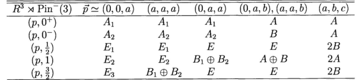
Table 2.4: Decomposition of continuum representations with non-zero moment into lattice representations.

R3 x Pin-(3)

f

-~ (0, 0, a) (a, a, a) (0, a, a) (0, a, b), (a, a, b) (a, b, c)

(p, 0+) A1 A1 A1 A A (p,O-) A2 A2 A2 B A (p, ) El E, E E 2B (p, 1) E2 E2 B1 D B2 A B 2A

(p, )

E

3

B1

B

22

E

E

2B

um

We use operators

ei

eO(v) (2.83)

with O given in Tab. 2.5. Here ni is a unit normal vector to one of the planes of reflection contained in the little group and Xy _{are spinors with definite helicity,}

"

3 X± = ±x+. (2.84)

The phases are chosen such that the reflection along n maps the spinors into each other, X_ = -i~i. 5-X+. Our choice of n is included in Tab. 2.3. As in the case of local pentaquark operators, the operators are defined such that all correlators are real.

2.9

Scattering states

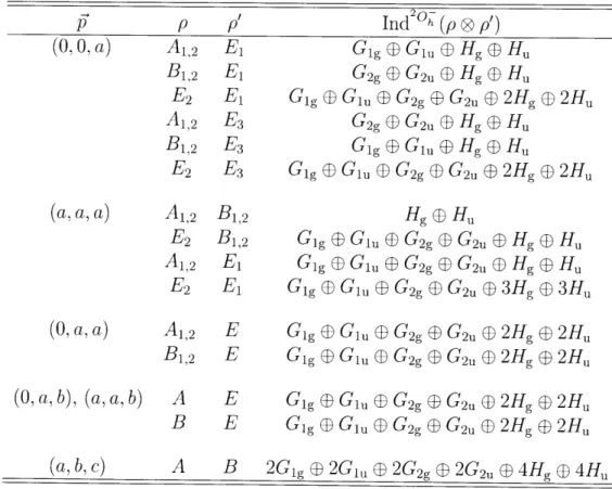
Once the masses of kaon and nucleon states are determined, we can make predictions for scattering states. We are interested in scattering states with total momentum zero and spin GI. The momentum-zero component of a product of two representations with non-zero momentum is the representation induced in 20 by the product of the

representations of the little group,

([p-, p) 0 (ý-, p') = (O, Ind20 (P p'))+... (f / 6).... (2.85)

The induced representations of all products of a bosonic and a fermionic state from Tab. 2.4 are given in Tab. 2.6. We need to consider all pairs that have a G1 in the

last column.

2.10

Operators for scattering states

We also attempt to measure scattering states directly (instead of the single-particle states they are made of) by using product operators. For negative parity, we couple

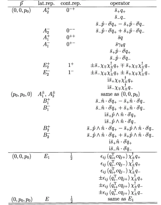
Table 2.5: Hadron operators for non-zero momentum. For E representations, sign alternatives + refer to the two helicity components of the representation.

P lat.rep. cont.rep. operator

(0, 0, po) A+ j+q+ 0- + sq_ s-:

i

p-q+ - s+±p

i

q-A 0-- s_-p. -•q+ + a+ . -q-A+ 0++ sq Al O+ - sY4q

s+p uq+

E 1+ sXrXt q, t E2

j

1- sxxQ+ s xt is+ XT

X

q+ i2-x

±x+q-(Po,Po, 0) A±, A± same as (0, 0, po)

B+ s_t. U q+ - s+• o q_

B-

s_-t *

5q+ + s++

f-q_

is+p A ft. aq+

ig_p A ft. aq

B+ s_- AnA a-- q+ - s+ A ft.

uq-B- g_i A ft - q + +9P A n a-q_ i+n - uq+ (0, O, po) E E (q2 +cqj+) X q+

Eij (q cqj )

Xt q+

Eij

(qi+cqj-) xt q -±Eij (q- ±tq+ ±Eij (qi+cq+)

xq-±ci (qT-cqj+) X

Table 2.6: Representations in 20h induced by product representations of the various little groups.

F P p' Ind 2 h(p ® p')

(0o, ,

a)

A

1

,

2

El

Gig Gu

E

Hg

@

Hu

B1,2 El G2g G2u (D Hg ( Hu

E2 E1 Gig D Glu D G2g q G2u D 2Hg D 2Hu

A1,2 E3 G2g

D

G2u e Hg ( Hu

B 1,2 E3 Gi, D Glu, _Hg ® _Hu

E2 E3 Gig D Glu e G2g ( G2u E 2Hg 1 2Hu

(a, a, a) A1,2 B1,2 Hg

a

Hu

E2 B1,2 Gig a Glu, G2g P G2u D Hg ( Hu A1,2 El Gig D Glu D Gg 2g G2u ( Hg ( Hu

E2 El Gig D GIu G₂g D G2u D 3Hg D 3Hu

(0, a, a) A1,2 E Gig D Glu D G₂g

aD

G2u 2Hg D 2Hu

B1,2 E Gig Glu, D G2g D G₂u E 2Hg D 2Hu

(O,

a,

b), (a, a, b) A

E

GigE Giu

G

2gO

G

2u

(

2Hg, 2Hu

B E Gig E Glu E G2g D G2u D 2Hg D 2Hu

(a, b, c) A B 2_GIg

_B

_2G1,

_D

_2G2g

_D

_2G

nucleon and kaon operators to G1u and isospin 0,

NKohh - cij

Y,m<k

UaONipc ()K, ,(+ ( (en + ek)) ,

Ki = 9+qi+ ,

Kn = +,'nqi+ ,

Nia = ckl (qk+cql+)qi+,a

are the unique K, K* and N operators with only large quark components. the operators have been chosen such that the correlators are real.

In momentum space,

NKooh =

>

e-iPmL/2i NI (pKj(-p) , g,m

NKOhh = e-i(Pm+Pk)L/2cij N i (pi K(-p g,m<k

NKohh ei(pm+Pk)L/- 2Eij auNi(p-fk(-p-. g,m<k

Since Pm = 27rnm/L, the phase factors are all ±1. Furthermore,

3

e-i(pm+pk)L/2 = ei(pl+P2+P3)L/2 e-ipmL/2

m<k

NKUOh = ij Nia (x)Kj

(+

-jKe) ,

x, m

NKo =O

j

apNip~(~K,

(*

+

ek),

NKOhh = ij i (£)K_i

(£+

-(e, + ek)) ,

g,m<k

(2.86)

(2.87)

(2.88)

(2.89) where (2.90) (2.91) (2.92) Again, (2.93) (2.94) (2.95) (2.96) (2.97)

The prefactor is ±1 for even/odd ni + n2 + n3. Therefore, the linear combinations

NKeven = NKooh + NKOhh , (2.98)

NKodd = NKOOh - NKOhh, (2.99)

NK00h + NKOhh = 2

E

e-ipmL/2Eij Nia (pj kj(-p) , (2.100)

geven,m

NK00h - NKOhh = 2 : e-ipmL/2Eij Nia (PpKj(-p•

(2.101)

fodd,m

(and similarly for NK*) contain only components with even resp. odd relative mo-mentum. Of course, due to nucleon-kaon interactions, all relative momenta mix. But we still expect these linear combinations to have good overlap with the cor-responding scattering states. In particular, '+' should have good overlap with the zero-momentum scattering state, and '-' with the state with ' = (0, 0, po).

We use translational and rotational invariance to replace the source operators by NK Oh = E•i Nia (03 Kj (L 3) , (2.102) NK h = Eij UlNip (0) KJ(fle 3) , (2.103)

NK hh Ei Nia ( 2)Kj ( 3 ) , (2.104)

NKhh = Eij UagpNi (-e ₂ )Kj,(ae3) . (2.105)

For positive parity, nucleon and kaon operators are coupled to Gig. If we only use positive parity nucleon and negative parity kaon operators, then this requires separations other than L/2. We use

NKOdo = Eij uamNi (Y)Kj ( ± 4aem) (2.106)

NK*A E ±cij N(x)Kjm

(•±

4a'm) , (2.107)

NKE = ijEmkn k i*(')K 3 ,(± 4a-m) , (2.108)

NKOdh = E -ij Or' Ni(Y)Kj (±4am + Lfk) ,

NK*AT = Ni( ,)Km -i (~14a e + k,

Odh ,k,

5,m n ,k,n,i

(2.109)

(2.110)

Chapter 3

Spectroscopic analysis

3.1

Equal-time correlation function and the

trans-fer matrix

We wish to extract information about energy eigenstates from the correlation matrix

C (t) = (I (t)II(0))

(3.1)

obtained from a lattice simulation. Here, HII are the operators from Eqs. (2.15)-(2.33), projected to zero spatial momentum. In order to talk about energy spectrum and eigenstates, we have to assume that a positive transfer matrix exists. Since this is not the case for the quenched theory, the analysis presented in this chapter is, strictly speaking, only approximate.

For t > 0, the above correlator is equal to a matrix element

Cij(t) = (vac

Hie-HfftIvac)

,

(3.2)

which is directly related to the spectrum of H.

For t = 0, the Euclidean correlator is no longer equal to the simple matrix element (3.2), but rather to the vacuum expectation value of the normal-ordered product of

Hi and IIH [47],

C(0)

=

(vac|N[HiUH ]lvac) ,

(3.3)

where normal ordering is defined by its action on quark operators: in a basis where

-yo = diag(1, 1, -1, -1),

N[()O()] =

{

()(YW) if oa, / = 1, 2

-qb3M(y)4a,(x) if

a , 3

= 3, 4.

(3.4)

In order to compute the matrix element (3.2) without normal-ordering, we have to sum the Euclidean expectation value over all contractions. In practice, this is achieved by replacing the naive quark propagator at equal time by the one corresponding to a non-normalordered expectation value,

Saia,bjp(_, t; -, t') = + CaiQ,bj/3(X, t; y, t') = where

(3.5)

(3.6)

depends on the fermion action. For the Wilson action [47],

Caia,bjO(*, t; Y, t') = --Si(1- -4)oaBd-1 (, Y)(t, t1)

with Bab(i, = 6abS(, 9) 3 -K Uiab + i, + U b((i)6( ,

i)

i=1 (3.7)

(3.8)

Sai

a,bj,(',

t; ', t')

Caia,bjO(/, t; , t1) ,

4aia(x, t)qýj

(Oy

t') N[qai, (x, t)bjp (y, t')]

3.2

A variation on the traditional variational method

In order to obtain approximate energy eigenstates, one usually solves the generalized eigenvalue problem

(3.9)

which is equivalent to the variational problem

6

(ue-

Htu)

6u

(u

e-Hto u) (3.10)

where u) = E 1i , vac)ui. The solutions for different eigenvalues are orthogonal with respect to C(to),

Unjiij(to )Umj = U if

An Am

.

We shall assume in the following that there are no degeneracies.

For large t, the lowest available energy eigenstate dominates the numerator in Eq. (3.10), so the solution

u"(to)- nt---0o limr un(t to) (3.12) maximizes the normalized overlap

I

(En-,l

(3.13)

under the constraint (3.11). It can be written as

) = I E -ar Ear)Mm~,1(E are-Hto E ar, (3.14)

where M is the (n - 1) x (n - 1) matrix with components

Mmm, = (Ear'le-Hto E") (

(3.11)

cij(t)

MUnj(t, to) = An (t, to) Cij (to) Uij(t, to) ,

and IE •₎

is the energy eigenstate projected to the variational space,

IE

var₎

= IIi)C(to)•l (HI j e-H t En) . (3.16)

Note that all quantities depend on to. The coefficients of the ground state solution, for instance, are

Uo(to) = NoC(to) 1(IIj Eo) (3.17)

where we have used that Eo) is an eigenstate of H.

In order to eliminate this dependence, we define coefficients

cni(t, to) - C(O)_lC(to)jkU nk(t, to) (3.18)

The large-t limit of Eo is to-independent,

(3.19)

&0.

-

_t-

lim

aoi(t,

to)

=

NoC(0)

l

₍

I j

_IE

_o).

O-*O0

They are the coefficients of the energy eigenstate projected to the variational space with respect to the natural metric Cij(0) = (IIlIlj₃),

(3.20)

lIIoi)a

=

Pn Eo),

where

PH = 1-i)(j 1(I1j • (3.21)

Note that, for to = 0, the new coefficients ₀oi are identical to the original uoi.

For excited states, an additional complication arises: the projected states u0), defined in (3.12), contain additional, to-dependent contributions from lower energy eigenstates. These introduce a to dependence in ",

(3.22)

ZIHi)an

= Pn

1

En)

+

PniEm)am(to).

This to dependence can be eliminated by orthogonalizing with respect to C(0),

ci (t, to) -- ni (t, to) - -miAm' 'CJk(O)ank ,(3.23)

where A is the (n - 1) x (n - 1) matrix with elements

Amm, = amiCij(O)amj (m,m' = 1,...,n - 1). (3.24)

The large-t limit c' of c satisfies

Sl

)nic = PnItEn) - Pl Em))B,• •(EmIPnIEn),, (3.25) where

Bm, = (EmlPnEm,) (m,m'= 1,..., n- 1). (3.26)

c' is to-independent and identical to ul(to=O). Explicitly,

lim cni(t, to) = lim uni(t, 0). (3.27)

t--+oo t-+oo

c, provides a means for computing the coefficient of the projected energy eigenstate PIE,) from the eigenvalue problem for any to. This turns out to be numerically advantageous in many cases.

Note that the components of PIE,), proportional to PniIEm) for m < n, which are lost in the orthogonalization appearing in (3.25), cannot be determined from the generalized eigenvalue problem even in principle. The corresponding components of the solution are determined solely from the requirement of orthogonality with respect to C(to). They are, of course, present only because of the truncation to the variational space. The full energy eigenstates are orthogonal.

Chapter 4

Calculational details

A preliminary version of the numerical calculation is reported in [44]. This work improves it in several ways. We still use quenched Wilson fermions with

f

= 6.0 and m, = 0.90 GeV(Ku,d = K = 0.1530) on same two spatial sizes 163 and 243, keeping Wuppertal and APE smearing parameters intact to allow for a direct comparison with the earlier results. In regards to the improvements, first off, we increase the time extent from 32 to 64 on both spatial volumes to catch longer plateaus, thus reducing both statistical and systematical errors on our system's energy levels. Sec-ondly, a lower light quark mass (r,d = 0.1558, m, = 0.55 GeV) was included in the analysis, with the strange quark mass kept fixed. Given the different variation of the pentaquark's, meson's, and baryon's masses with the light quark mass, this offers the potential to further distinguish localized states of the pentaquark system from scattering states of a baryon and a meson. Finally, the number of configurations was increased to 4672 on a 163 x 64 lattice (only the heavier quark mass) and 1024 on a 243 x 64 lattice (both quark masses), amounting to a total of 3.2 terabytes in propagators alone.

To improve the overlap of interpolating operators with low-lying energy eigen-states, we employ Wuppertal smearing, a well-established method based on the idea of increasing the spatial extent of the source to approximate that of a typical hadron. The quark field q(, t) is replaced in the interpolating operators with the smeared