HAL Id: hal-01300699
https://hal.archives-ouvertes.fr/hal-01300699
Submitted on 11 Apr 2016
HAL is a multi-disciplinary open access
archive for the deposit and dissemination of
sci-entific research documents, whether they are
pub-lished or not. The documents may come from
teaching and research institutions in France or
abroad, or from public or private research centers.
L’archive ouverte pluridisciplinaire HAL, est
destinée au dépôt et à la diffusion de documents
scientifiques de niveau recherche, publiés ou non,
émanant des établissements d’enseignement et de
recherche français ou étrangers, des laboratoires
publics ou privés.
Evolving Neural Networks That Are Both Modular and
Regular: HyperNeat Plus the Connection Cost
Technique
Joost Huizinga, Jean-Baptiste Mouret, Jeff Clune
To cite this version:
Joost Huizinga, Jean-Baptiste Mouret, Jeff Clune. Evolving Neural Networks That Are Both Modular
and Regular: HyperNeat Plus the Connection Cost Technique. GECCO ’14: Proceedings of the 2014
Annual Conference on Genetic and Evolutionary Computation, ACM, 2014, Vancouver, Canada.
pp.697-704. �hal-01300699�
To appear in: Proceedings of the Genetic and Evolutionary Computation Conference. 2014
Evolving Neural Networks That Are Both Modular and
Regular: HyperNeat Plus the Connection Cost Technique
Joost Huizinga
Evolving AI Lab Department of Computer Science University of Wyoming [email protected]Jean-Baptiste Mouret
ISIR, Université Pierre etMarie Curie-Paris 6 CNRS UMR 7222 Paris, France [email protected]
Jeff Clune
Evolving AI Lab Department of Computer Science University of Wyoming [email protected]ABSTRACT
One of humanity’s grand scientific challenges is to create ar-tificially intelligent robots that rival natural animals in intel-ligence and agility. A key enabler of such animal complexity is the fact that animal brains are structurally organized in that they exhibit modularity and regularity, amongst other attributes. Modularity is the localization of function within an encapsulated unit. Regularity refers to the compressibil-ity of the information describing a structure, and typically involves symmetries and repetition. These properties im-prove evolvability, but they rarely emerge in evolutionary algorithms without specific techniques to encourage them. It has been shown that (1) modularity can be evolved in neural networks by adding a cost for neural connections and, sepa-rately, (2) that the HyperNEAT algorithm produces neural networks with complex, functional regularities. In this pa-per we show that adding the connection cost technique to HyperNEAT produces neural networks that are significantly more modular, regular, and higher performing than Hyper-NEAT without a connection cost, even when compared to a variant of HyperNEAT that was specifically designed to en-courage modularity. Our results represent a stepping stone towards the goal of producing artificial neural networks that share key organizational properties with the brains of natu-ral animals.
Categories and Subject Descriptors
I.2.6 [Artificial Intelligence]: Learning—Connectionism and neural nets
Keywords
Artificial Neural Networks; Modularity; Regularity; Hyper-NEAT; NSGA-II
Permission to make digital or hard copies of all or part of this work for personal or classroom use is granted without fee provided that copies are not made or distributed for profit or commercial advantage and that copies bear this notice and the full citation on the first page. Copyrights for components of this work owned by others than the author(s) must be honored. Abstracting with credit is permitted. To copy otherwise, or republish, to post on servers or to redistribute to lists, requires prior specific permission and/or a fee. Request permissions from [email protected].
GECCO’14, July 12–16, 2014, Vancouver, BC, Canada.
Copyright is held by the owner/author(s). Publication rights licensed to ACM. ACM 978-1-4503-2662-9/14/07 ...$15.00.
http://dx.doi.org/10.1145/2576768.2598232.
1. INTRODUCTION
An open and ambitious question in the field of evolution-ary robotics is how to produce robots that possess the intel-ligence, versatility, and agility of natural animals. A major enabler of such complexity in animals lies in the fact that their bodies and brains are structurally organized in that they exhibit modularity and regularity, amongst other at-tributes [22, 30].
A network is considered modular if it contains groups of highly interconnected nodes, called modules, which are only sparsely connected to nodes outside the module [8, 17, 22]. In addition to such topological modularity, an even stronger case for modularity can be made if such topological modules correspond to the performance of sub-functions, a property called functional modularity [22].
Theoretical and empirical evidence suggests that modular-ity speeds up evolvabilmodular-ity, which is the rate of evolutionary adaptation [1, 8, 17–19]. Modularity improves evolvability by allowing building blocks (modules) to be rewired for new functions and—because the e↵ects of mutations tend to be confined within a module—by allowing evolution to tinker with one module without global e↵ects [17].
Regularity can be defined as: “the compressibility of the description of the structure” [22]; as a structure becomes more regular, less information is required to describe it. Common forms of regularity include repetition, symmetry and self-similarity. It has been shown that regularity im-proves both performance and evolvability [5, 7, 14, 15], and increasingly does so on more regular problems [10]. Legged locomotion, for example, can greatly benefit from the reuse of information [5, 10, 14–16].
Despite the advantages of modularity and regularity, these properties do not naturally emerge in evolutionary algo-rithms without special techniques to encourage them [8–10, 17]. While these properties enhance evolvability and ulti-mately performance, such long-term advantages do not typ-ically grant an immediate fitness boost to individuals that exhibit them. Evolution has been shown to forgo long-term benefits in performance and evolvability if there is no short-term benefit [7, 37, 38].
Encouraging the evolution of modularity has been a long-standing interest in the field, yielding a variety of strategies to promote it [8,12,14,15,17,31,32,35,36]. One general strat-egy is to design developmental systems featuring encodings biased towards modular structures [14, 15, 31, 32, 35]. While e↵ective, these heavily biased encodings often produce
net-works that adhere very closely to a specific structure, leaving little room to adapt when circumstances require a di↵erent topology. Another method was demonstrated by Kashtan and Alon [17], who showed that alternating environments with modularly varying goals can give rise to modular net-works. Unfortunately, it can be difficult to define modularly varying goals for many tasks. Moreover, the frequency of al-ternating between these environments must be finely tuned for the e↵ect to emerge [8, 12]. Espinosa-Soto and Wag-ner [12] found that modularity can be evolved by selecting for a new task while retaining selection for previously ac-quired functionalities. However, it is non-trivial to decide on a sequence of sub-tasks that will eventually provide a complex, functionally modular solution to a specific task.
In this paper we will build upon a di↵erent, recently pub-lished method that yields the evolution of modular networks. In 2013, Clune, Mouret and Lipson showed that applying a cost for network connections leads to modular networks [8], and does so in a wider range of environments than a previous leading method [17]. This connection-cost technique (CCT) is biologically plausible, as many connection costs exist in natural networks, such as the cost to build and maintain connections, slower propagation through long connections, and the physical space occupied by long connections [30]. Connection costs may thus help explain the ubiquitous mod-ularity found in natural networks [8, 30]. Furthermore, the CCT is computationally inexpensive and can be easily in-corporated into the fitness of any evolutionary algorithm, especially multi-objective algorithms [11].
The most common method for producing regular networks is to use a generative encoding (also called an indirect or de-velopmental encoding) [10, 14–16, 27, 29, 31]. The encoding of an individual defines how its genotype is mapped to its phenotype, and a generative encoding implies an indirect mapping such that elements in the genotype might describe more than just a single element in the phenotype. Gener-ative encodings are often based on natural developmental systems, such as gene regulatory networks, cell division, or chemical gradients, making them more biologically plausible than direct encodings [29]. In generative encodings, compact genomes describe a much larger phenotype via the reuse of genomic information, giving rise to regular structures. In fact, if we consider the genotype as a compression of the phenotype, large phenotypes encoded by small genotypes are regular by definition [22].
To generate regularity we employ the HyperNEAT [27] algorithm, which encodes neural networks with a generative encoding called Compositional Pattern Producing Networks (CPPNs) [26]. CPPNs produce spatial patterns that ex-hibit regularity with variation (Fig. 1a). These spatial pat-terns define the connectivity across the geometric layout of nodes, enabling HyperNEAT to produce networks that ex-hibit structural regularity [9]. This paper demonstrates that the combination of HyperNEAT with the Connection Cost Technique –HyperNEAT-CCT– produces networks that are both modular and regular.
2. METHODS
2.1 HyperNEAT
To generate a network, HyperNEAT requires a geometric layout of nodes (see Fig. 1b-d for the layouts for problems in this paper). Given one of these layouts and a CPPN, the
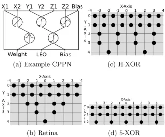
(a) Example CPPN (c) H-XOR
(b) Retina (d) 5-XOR
Figure 1: Example CPPN and geometric layouts. (a) A CPPN example (see section 2.1). (b) Geometric lay-out for the Retina Problem. (c) Geometric laylay-out for the H-XOR problem. (d) Geometric layout for the 5-XOR problem. Note that, the z coordinates of all nodes are 0. connectivity of a network is determined by supplying the x, y, and, z coordinates of two neurons as inputs to the CPPN, after which the weight of the connection between those neu-rons is set to the weight output of the CPPN (Fig. 1a). To set the biases of neurons, the x, y and z coordinates of a single node are supplied to the CPPN together with a null position for the other inputs, and the bias is read from a separate bias output node (Fig. 1a).
Because it has been demonstrated that the original Hyper-NEAT has trouble creating modular networks [4], we have implemented HyperNEAT with the Link-Expression Out-put (LEO) [36], an additional outOut-put neuron determining whether connections are expressed (Fig. 1a). This extension allows HyperNEAT to separate network connectivity from weight patterns, enhancing its ability to evolve sparsely con-nected, yet functional, sub-units. Connecting a Gaussian seed to LEO further increases HyperNEAT’s ability to pro-duce modular networks [36].
The Gaussian seed consists of an additional hidden node with a Gaussian activation function, added to the network upon initialization. This node is connected to two inputs by one inhibitory and one excitatory connection, such that their sum represents the di↵erence along one axis. Because the Gaussian activation function produces strong activations only for values close to 0, it will ‘fire’ only when distances between nodes are short, thus encouraging shorter connec-tions, which may help in discovering modular solutions [36]. However, by planting the Gaussian seed inside the CPPN, there is no guarantee that the seed will be preserved through-out evolution. Whenever there is no immediate benefit for shorter connections, which may occur at any point in a run, the Gaussian seed might disappear completely from the pop-ulation. We believe that, due to its persistence as a selec-tion pressure, the CCT will generally outperform the locality seed. That is because there exist many situations in which the advantages of short connections are not immediate while solving problems in challenging or changing environments. To test that hypothesis we include a treatment featuring HyperNEAT, LEO, and the Gaussian seed.
In our implementation the seed is exclusively employed for the x inputs, which was reported to be the most successful variant [36]. The weights from the input to the Gaussian seed are 0.6 and 0.6, respectively. The LEO node starts with a sigmoid activation function (a hyperbolic tangent) and a negative bias ( 1). A link is expressed when the LEO node returns a value 0, which provides a behavior similar to the step function used in [36].
HyperNEAT evolves CPPNs genomes via the NeuroEvo-lution of Augmenting Topologies (NEAT) algorithm [28]. The three important parts of the NEAT algorithm are (1) an intelligent method for crossover between networks, (2) protecting diversity through speciation and (3) complexifi-cation, which means starting with networks that have few nodes and connections, and adding them across evolution-ary time. In this paper we have implemented HyperNEAT within the PNSGA algorithm from [8], which is programmed within the Sferes21 platform [23]. The resulting algorithm
di↵ers from NEAT in two ways. First, speciation, which encourages genomic diversity in NEAT, is replaced by a be-havioral diversity objective, an adaptation employed in sev-eral other publications [20, 33]. Second, crossover has been removed for simplicity. We follow previous publications by the authors of HyperNEAT in maintaining the name Hyper-NEAT to algorithmic variants that have its key components (e.g. CPPNs, complexification, and diversity) [20, 33].
2.2 Experiments
There are four di↵erent treatments: (1) HyperNEAT, (2) HyperNEAT with the Gaussian Seed (HyperNEAT-GS) [36], (3) HyperNEAT with the Connection Cost Technique (HyperNEAT-CCT), and (4) a direct encoding with the Con-nection Cost Technique (DirectEncoding-CCT), which is the main algorithm from [8]. Each HyperNEAT treatment fea-tures LEO (explained above). All treatments are evolved according to the same evolutionary algorithm described in section 2.3, and every treatment optimizes at least two ob-jectives: performance on the test problem and behavioral diversity. Treatments employing CCT add minimizing con-nection costs as a third objective.
Behavioral diversity of an individual is calculated by stor-ing the output for every possible input in a binary vector (< 0 is false, 0 is true) and then taking the average Ham-ming distance to the binary vector of all other individuals in the population. The connection-cost is calculated as the sum of squared lengths of all connections in the phenotype [8].
2.3 Evolutionary Algorithm
We incorporate the CCT into the multi-objective PNSGA algorithm [8], an extended version of NSGA-II [11]. These algorithms optimize individuals on several tasks at once, and try to preserve and select for all individuals that have some unique trade-o↵ between between objectives, such as being very good at one task but terrible at the others, or being av-erage at all tasks. PNSGA extends NSGA-II by assigning a probability to an objective, which determines the frequency that this objective will factor into selection. By assigning a lower probability to the connection cost objective, we can implement the intuition that performance on the task is more important than a low connection cost. For these
ex-1All of the source code used to perform these experiments
is available on EvolvingAI.com.
periments, following [8], the probability of the connection cost factoring into a fitness comparison is 25%.
The population is initialized with randomly generated, fully connected networks without hidden nodes, as is pre-scribed for NEAT [28]. Parents are chosen via tournament selection (tournament size of 2), where the winner is the one that dominates the other, with ties broken randomly.
Parents are copied and the copies are mutated follow-ing [8]. The mutation operators: add connection (9%), re-move connection (8%), add node (5%), and rere-move node (4%), are executed at most once. Change weight (10%) and, for CPPNs, change activation function (10%) mutations are performed on a per connection and per node basis. Mutation rates were chosen as the result of a preliminary parameter sweep for high performance. For CPPN-based treatments the activation functions are randomly selected from the fol-lowing set: Gaussian, linear, sigmoid and sine. Biases are handled by an additional input that always has an activa-tion of 1, meaning the connecactiva-tion between a node and this input determines the bias for that node.
Survivors were selected from the mixed population of o↵-spring and parents. For all experiments the population size was 1000 and the only stopping condition was the maximum number of generations, which was either 25000 or 50000, de-pending on the problem.
2.4 Test problems
We have tested all treatments on three modular and reg-ular problems from [8]: the Retina Problem (originally introduced in [17]), the 5-XOR problem, and the Hier-archical XOR problem.
The Retina Problem simulates a simple retina that re-ceives visual input from 8 pixels (Fig. 2a). The left and right halves of the retina may each contain a pattern of interest known as an “object”. The patterns, shown in figure 2b, are flattened versions of those from [8] and are defined such that each pattern has a mirror image on the other side of the retina, providing at least one symmetry that can be discov-ered. The network is tested on all 256 possible patterns and the task for the network is to indicate whether there is (> 0) or is not (< 0) an object present at both the left and the right side of the retina. Note that, while the problem is modu-larly decomposable, there also exist perfect-performing, non-modular solutions [8, 17].
(a) Retina (b) Retina objects
(c) 5-XOR
(d) H-XOR Figure 2: Experimental Problems. (a) The general structure of the Retina Problem, where the network has to answer whether there is both a left and a right object present. (b) The patterns that count as objects for the Retina Problem. (c) The H-XOR problem, consisting of 2 identical, hierarchically nested XOR problems. (d) The 5-XOR problem, which contains 5 separate XOR problems.
The 5-XOR problem (Fig. 2c) includes five independent XOR problems that a network must solve in parallel. Per-formance on this task is the average perPer-formance over all five XOR tasks. The problem has regularity because of the repeated XORs and it is modularly decomposable because each XOR can be solved separately.
The Hierarchical XOR problem (H-XOR) (Fig. 2d) consist of two separable, hierarchically nested XOR lems (the XOR of two XORs). As with the 5-XOR prob-lem, separability and repetition make that both modularity and regularity are expected to be beneficial in this problem.
2.5 Metrics and Visualizations
When reporting the performance across runs we always consider the ‘best’ individual of the population, where ‘best’ means the first individual when sorting on performance first and modularity second. Ties are broken arbitrarily.
The structural modularity of our networks is measured by the widely-used modularity Q-score [24]. For functional modularity we use two measures from [8]: modular decom-position and sub-problems solved. To calculate modular de-composition we split the network to maximize modularity, as described in [24], with the maximum number of allowed splits equal to the number of sub-problems, and test whether inputs corresponding to di↵erent sub-problems end up in di↵erent modules. To calculate the number of sub-problems solved we check, for every sub-problem, whether there exists a node in the network that linearly separates the positive and negative classes of that sub-problem. If such a node exists the sub-problem is considered solved.
Following [8], we visualize modularity by moving nodes to the location that minimizes the summed length of their con-nections, while holding inputs and outputs fixed (Fig. 3c). This optimal neural placement (ONP) visualization is in-spired by the fact that neurons in some natural organisms are located optimally to minimize the summed length of the connections between them [2, 3]. Nodes in the ONP visual-izations are colored according to the best modular split. The maximum number of splits performed depends on the prob-lem: the Retina Problem and H-XOR problems are split in two parts, while the 5-XOR problem is split in 5 parts. Nodes that solve one of the sub-problems are depicted with a large colored border surrounding them. Because modularity di↵erences are not visually apparent at the lower and higher levels (all treatments produce some modular and some non-modular networks) the networks within each treatment are sorted according to their modularity and those around the middle of this list are depicted in this paper.
As mentioned in section 1, regularity can be defined as the compressibility of the data describing a structure. How-ever, since this minimum description length is impossible to calculate exactly [21], we approximate the regularity by compressing the network using the Lempel-Ziv-Welch com-pression algorithm. To approximate regularity, we write the network weights and biases to an ASCII string, compress it, and test by which fraction the string size was reduced. Be-cause order matters, we repeat this process for 500 di↵erent permutations of the weights and biases and take the average as the regularity value.
When visualizing regularity we leave nodes in their ac-tual geometric locations so as not to distort regularities (e.g. Fig. 4). In this visualization we color excitatory connections green and inhibitory connections red. The width of the
con-nection indicates the strength of that concon-nection. Similarly, we depict the bias of each node as a circle inside each node, where green circles indicate a positive bias, red circles indi-cate a negative bias, and the size of the circle indiindi-cates the strength of the bias.
Statistical tests are performed with the Mann-Withney-U rank sum test, unless otherwise specified. Shaded areas in graphs represent 95% bootstrapped confidence intervals of the median, generated by sampling the data 5000 times. Tri-angles below graphs indicate when values for HyperNEAT-CCT are significantly higher than for the treatment with the corresponding symbol and treatment color (p < 0.05).
3. RESULTS
3.1 The Retina Problem
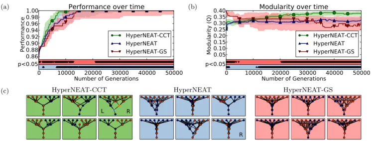
In the retina experiment, the performance of HyperNEAT-CCT is significantly higher at nearly every generation than both HyperNEAT and HyperNEAT-GS (Fig. 3a); even af-ter the medians of all treatments have reached perfect per-formance, lower-performing runs in the HyperNEAT and HyperNEAT-GS treatments make those treatments perform significantly worse than HyperNEAT-CCT. In terms of mod-ularity, the level for HyperNEAT hardly changes over time, while the modularity of HyperNEAT-CCT progressively in-creases; the di↵erence becomes significant after 12000 gen-erations (Fig. 3b). The modularity of HyperNEAT-GS, on the other hand, spikes during the first few generations, but then it decreases over time to a significantly lower level than HyperNEAT-CCT (Fig. 3b). This behavior is evidence for our hypothesis that the Gaussian seed may not be an e↵ec-tive way to promote modularity in cases where there is no immediate fitness benefit.
To examine functional modularity we look at the best net-works produced after 50000 generations. Our test for prob-lem decomposition, which in this case is having the inputs for the left and right sub-problems in di↵erent modules (sec-tion 2.5), shows that 75% of the HyperNEAT-CCT runs are left-right modular, which is higher than HyperNEAT, for which 64% of the networks are left-right modular, but the di↵erence is not significant (p = 0.124 Fisher’s exact test). In addition, when considering the number of sub-problems solved (section 2.5), HyperNEAT-CCT networks solve an average of 0.67 (out of 2) sub-problems, which is significantly (p = 0.024) higher than HyperNEAT networks, which solve an average of 0.41 sub-problems.
The di↵erences in modularity are also visually apparent (Fig. 3c). The networks of HyperNEAT-CCT look more modular, demonstrate left-right modularity more often, and have more nodes that solve sub-problems than the Hyper-NEAT and HyperHyper-NEAT-GS networks.
The reason HyperNEAT-CCT performs better is proba-bly because the problem is modular. Additionally, by guid-ing evolution towards the space of networks with fewer con-nections, fewer weights need to be optimized. As analy-ses in [8] revealed, the reason treatments that select for performance alone do not produce modularity despite its benefits is because the benefits of modularity come in the long term, whereas selection acts on immediate fitness ben-efits. Interestingly, most of the modularity increases occur after the majority of HyperNEAT-CCT runs have achieved near-perfect performance. That is likely because once per-formance is perfect, or nearly so, the only way a network
(a) (b)
(c) HyperNEAT-CCT HyperNEAT HyperNEAT-GS
Figure 3: Results for the Retina Problem. HyperNEAT-CCT significantly (a) outperforms and (b) has higher mod-ularity than both HyperNEAT and HyperNEAT-GS. (c) ONP visualizations (see section 2.5) for networks 54 to 60 (out of 100) for HyperNEAT and HyperNEAT-CCT and networks 27 to 33 (out of 50) for HyperNEAT-GS (sorted on modularity). Colored rings indicate neurons that solve the right (orange) and left (blue) sub-problems. HyperNEAT-CCT networks are visually more modular, exhibit left-right modularity more often, and solve significantly more sub-problems than HyperNEAT or HyperNEAT-GS networks.
(a) (b) HyperNEAT-CCT
DirectEncoding-CCT
Figure 4: CCT networks are more regular than DirectEncoding-CCT networks. (a) HyperNEAT-CCT networks compress significantly more (p < 0.00001). (b) Four perfectly-performing networks with the highest modularity scores from HyperNEAT-CCT and DirectEncoding-CCT. All four networks of HyperNEAT-CCT show some form of symmetry with variation, including switching excitatory and inhibitory connections. The DirectEncoding-CCT networks are irregular. can be selected over others is by reducing connection costs,
which tends to increase modularity [8].
While the results of HyperNEAT-GS are lower than ex-pected, the figures shown are for the highest-performing ver-sion of it that we found after experimenting with its key parameters (Fig 4a, b and c). Initially we ran HyperNEAT-GS with the default settings for the Gaussian seed [36] and a negative bias on the LEO output of 2, which resulted in fewer connections by enforcing stronger spatial constraints. After analyzing our results, we hypothesized that the poor performance of HyperNEAT-GS might have been because the distances between our nodes are greater than in [36], so we switched to settings (described in section 2.2) that compensate for the increased distances. These settings sig-nificantly improved performance (p < 0.05 for most gener-ations), but did not improve modularity. We subsequently changed the bias from 2 to 1, which is more suitable when applying locality to only a single axis, and while this
change improved modularity to the level reported in Fig. 3b, the overall results are still worse than those reported in [36]. This di↵erence in performance is likely due to di↵erences in the evolutionary algorithm (section 2.1) and in the prob-lem definition (in [36] the sub-probprob-lems did not have to be combined into a single answer).
Since changing its seed improved the performance ob-tained by HyperNEAT-GS, it is possible that it can be im-proved to a level where it outperforms HyperNEAT-CCT. However, the weights of the Gaussian seed were free to evolve, yet evolution was unable to adapt the seed to im-prove either performance or modularity, which shows that HyperNEAT-GS can fail to produce modularity in absence of direct rewards.
The di↵erences between the treatments with and without a connection-cost are not as pronounced as those demon-strated by Clune, Mouret and Lipson [8], indicating that the beneficial e↵ects of CCT on HyperNEAT are not as great as
was the case for the direct encoding. The reason for this is probably that HyperNEAT, even with the Link-Expression Output, has trouble pruning individual connections.
Comparing HyperNEAT-CCT with DirectEncoding-CCT (the main algorithm from [8]), the direct encoding is sig-nificantly higher performing in early generations and signif-icantly more modular throughout evolution. The indirect encoding of HyperNEAT seems to struggle more with the irregularities of this problem and is not as good at pruning connections. That is expected, since removing connections in the direct encoding is easy compared to doing so in Hy-perNEAT, which has to adapt the patterns produced by the LEO node such that it cuts o↵ the redundant parts while keeping the rest of the network intact.
A main advantage of HyperNEAT is its ability to produce regular patterns [9, 10, 27]. Compression tests (see methods, section 2.5) reveal that HyperNEAT-CCT networks are sig-nificantly more regular than the DirectEncoding-CCT (Fig-ure 4): the direct encoding with CCT becomes 38% smaller upon compression, but HyperNEAT-CCT compresses fur-ther down by 43%, making it significantly more compress-ible (p < 0.00001). Thus, HyperNEAT-CCT networks are regular in addition to being modular.
The regularity of HyperNEAT-CCT is also visually ap-parent (Fig. 4b). In many of its networks, the left side is mirrored on the right side, even though the signs of the con-nections are sometimes switched. Other networks feature alternating or mirrored patterns in the biases or connec-tions. While HyperNEAT-CCT networks also exhibit some clear variations in each of its patterns, on balance they are much more regular than the DirectEncoding-CCT networks (Fig. 4b), which do not show any discernible patterns.
3.2 The 5-XOR and H-XOR problems
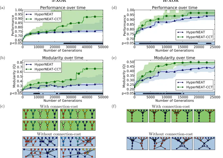
On the 5-XOR problem the treatments di↵er only slightly until after 25000 generations, where the performance and modularity of HyperNEAT-CCT becomes significantly bet-ter than HyperNEAT (Fig. 5a,b). The visual di↵erence in modularity is also clear for networks of intermediate modu-larity (Fig. 5c); HyperNEAT-CCT networks perfectly divide the problem into five individual networks while the networks produced by HyperNEAT are entangled.
On the H-XOR problem, HyperNEAT-CCT significantly outperforms HyperNEAT in both performance and modular-ity for most of the first 15000 generations (Fig. 5d,e). Hyper-NEAT eventually catches up, erasing the significant di↵er-ences. Network visualizations reveal clear examples where HyperNEAT-CCT networks modularly decompose the prob-lem, whereas HyperNEAT networks have not managed to disentangle the left and right problems (Figure 5f).
Due to computational and time constraints, we did not test HyperNEAT-GS on the 5-XOR and H-XOR problem. Given the results presented in section 3.1, it is likely that HyperNEAT-GS would underperform HyperNEAT and Hy-perNEAT-CCT. Also, because splitting the sub-problems is necessary to obtain perfect performance on these problems, there is no need to test for sub-problems solved as this will be directly reflected in performance.
4. FUTURE WORK
While we have shown the advantages of HyperNEAT-CCT on simple diagnostic problems, the real power of this method lies in its ability to create large-scale, modular networks.
HyperNEAT can create functional neural networks with mil-lions of connections, but the networks and tasks performed were simple [13, 27]. In future research we will increase the scale of networks that have both regularity and modular-ity and test whether these properties improve the abilmodular-ity to perform more complex tasks.
An other area to explore is to allow HyperNEAT to evolve the number and geometric location of its hidden neurons [25]. Because the patterns of neural connectivity HyperNEAT produces depend on the geometric location of nodes [9], adding the CCT to Evolvable-Substrate HyperNEAT [25] may further increase HyperNEAT’s ability to create func-tional neural modularity and could reduce the need for users to create geometric node layouts that encourage the appro-priate modular decomposition of problems.
Lastly, a recent technique showed that the regular pat-terns produced by a generative encoding, such as Hyper-NEAT, aids the learning capabilities of networks [34]. We will combine our method with intra-life learning algorithms to investigate whether learning is improved when it occurs in structurally organized neural networks. Such learning may also ameliorate HyperNEAT’s inability to cope with irregu-larity [6, 10].
5. CONCLUSION
One strategy to make robots more intelligent and agile is to evolve neural network controllers that emulate the struc-tural organization of animal brains, including their modular-ity and regularmodular-ity. Because these properties do not naturally emerge in evolutionary algorithms, some techniques have to be employed to encourage them to evolve. We have demon-strated how HyperNEAT with the connection-cost technique (HyperNEAT-CCT) can evolve networks that are both mod-ular and regmod-ular, which increases performance on modmod-ular, regular problems compared to both the default HyperNEAT algorithm and a variant of HyperNEAT specifically designed to encourage modularity. We have also shown that networks produced by HyperNEAT-CCT are more regular than net-works produced by adding the CCT to a direct encoding.
While other methods that lead to modular and regular networks exist, this work demonstrates a powerful, general way to promote modularity in the HyperNEAT algorithm, which has recently become one of the leading generative en-codings due to its ability to produce complex regularities, evolve extremely large-scale neural networks, and exploit the geometry of problems. Our work thus merges separate lines of research into evolving regularity and modularity, allowing them to be combined into a potentially powerful algorithm that can produce large-scale neural networks that exhibit key properties of structural organization in animal brains. Our work thus represents a step towards the day in which we can evolve computational brains that rival natural brains in complexity and intelligence.
6. ACKNOWLEDGMENTS
We thank Kai Olav Ellefsen and the members of the Evolv-ing AI Lab. JBM is supported by an ANR young researchers grant (Creadapt, ANR-12-JS03-0009).
5-XOR H-XOR
(a) (d)
(b) (e)
(c) With connection-cost (f) With connection-cost
Without connection-cost Without connection-cost
Figure 5: A Connection Cost Also Increases Modularity and Regularity on the 5-XOR and H-XOR Problems. (a) Median performance over time for the 5-XOR experiment. HyperNEAT-CCT performs significantly better than Hyper-NEAT after 25000 generations. ( b) Median modularity over time for the 5-XOR problem. HyperHyper-NEAT-CCT is significantly more modular than HyperNEAT after around 22000 generations (and for periods prior). (c) A comparison of 5-XOR networks 18-22 (sorted on modularity) showing ONP visualizations (see methods). HyperNEAT-CCT networks decompose the problem into the appropriate five modules while HyperNEAT without a connection cost makes unnecessary connections between the separate XOR problems. (d) On the H-XOR problem, HyperNEAT-CCT performs significantly better than HyperNEAT for most of the run. (e) HyperNEAT-CCT is significantly more modular for most early generations before HyperNEAT catches up. (f ) A visual comparison of H-XOR networks 24-28 (sorted on modularity) showing ONP visualizations (see methods). HyperNEAT-CCT splits the problem perfectly while HyperNEAT makes unnecessary connections between the left and the right problems.
7. REFERENCES
[1] S.B. Carroll. Chance and necessity: the evolution of morphological complexity and diversity. Nature, 409(6823):1102–1109, 2001.
[2] C. Cherniak, Z. Mokhtarzada, R. Rodriguez-Esteban, and K. Changizi. Global optimization of cerebral cortex layout. Proceedings of the National Academy of Sciences, 101(4):1081–6, January 2004.
[3] D.B. Chklovskii, T. Schikorski, and C.F. Stevens. Wiring optimization in cortical circuits. Neuron, 34(3):341–347, 2002.
[4] J. Clune, B.E. Beckmann, P.K. McKinley, and C. Ofria. Investigating whether HyperNEAT produces modular neural networks. In Proceedings of the
Genetic and Evolutionary Computation Conference, pages 635–642. ACM, 2010.
[5] J. Clune, B.E. Beckmann, C. Ofria, and R.T. Pennock. Evolving coordinated quadruped gaits with the HyperNEAT generative encoding. In Proceedings of the IEEE Congress on Evolutionary Computation, pages 2764–2771, 2009.
[6] J. Clune, B.E. Beckmann, R.T. Pennock, and C. Ofria. HybrID: A Hybridization of Indirect and Direct Encodings for Evolutionary Computation. In Proceedings of the European Conference on Artificial Life, 2009.
[7] J. Clune, D. Misevic, C. Ofria, R.E. Lenski, S.F. Elena, and R. Sanju´an. Natural selection fails to
optimize mutation rates for long-term adaptation on rugged fitness landscapes. PLoS Computational Biology, 4(9):e1000187, 2008.
[8] J. Clune, J-B. Mouret, and H. Lipson. The
evolutionary origins of modularity. Proceedings of the Royal Society B, 280(20122863), 2013.
[9] J. Clune, C. Ofria, and R.T. Pennock. The sensitivity of HyperNEAT to di↵erent geometric representations of a problem. In Proceedings of the Genetic and Evolutionary Computation Conference, pages 675–682, 2009.
[10] J. Clune, K.O. Stanley, R.T. Pennock, and C. Ofria. On the performance of indirect encoding across the continuum of regularity. IEEE Transactions on Evolutionary Computation, 15(4):346–367, 2011. [11] K. Deb, A. Pratap, S. Agarwal, and T.A.M.T.
Meyarivan. A fast and elitist multiobjective genetic algorithm: Nsga-ii. Evolutionary Computation, IEEE Transactions on, 6(2):182–197, 2002.
[12] C. Espinosa-Soto and A. Wagner. Specialization can drive the evolution of modularity. PLoS
Computational Biology, 6(3):e1000719, 2010. [13] J. Gauci and K.O. Stanley. Generating large-scale
neural networks through discovering geometric regularities. In Proceedings of the Genetic and Evolutionary Computation Conference, pages 997–1004. ACM, 2007.
[14] G.S. Hornby, H. Lipson, and J.B. Pollack. Generative representations for the automated design of modular physical robots. IEEE Transactions on Robotics and Automation, 19(4):703–719, 2003.
[15] G.S. Hornby and J. B. Pollack. Evolving L-systems to generate virtual creatures. Computers & Graphics, 25(6):1041–1048, December 2001.
[16] B. Inden, Y. Jin, R. Haschke, and H. Ritter.
Exploiting inherent regularity in control of multilegged robot locomotion by evolving neural fields. 2011 Third World Congress on Nature and Biologically Inspired Computing, pages 401–408, October 2011.
[17] N. Kashtan and U. Alon. Spontaneous evolution of modularity and network motifs. Proceedings of the National Academy of Sciences, 102(39):13773–13778, September 2005.
[18] N. Kashtan, E. Noor, and U. Alon. Varying
environments can speed up evolution. Proceedings of the National Academy of Sciences,
104(34):13711–13716, August 2007.
[19] C.P. Klingenberg. Developmental constraints, modules and evolvability. Variation: A central concept in biology, pages 1–30, 2005.
[20] J. Lehman, S. Risi, D.B. D’Ambrosio, and K.O. Stanley. Encouraging reactivity to create robust machines. Adaptive Behavior, 21(6):484–500, August 2013.
[21] M. Li. An introduction to Kolmogorov complexity and its applications. Springer, 1997.
[22] H. Lipson. Principles of modularity, regularity, and hierarchy for scalable systems. Journal of Biological Physics and Chemistry, 7(December):125–128, 2007. [23] J-B. Mouret and S. Doncieux. Sferes v2: Evolvin’ in
the multi-core world. IEEE Congress on Evolutionary Computation, (2):1–8, July 2010.
[24] M.E.J. Newman. Modularity and community structure in networks. Proceedings of the National Academy of Sciences, 103(23):8577–8582, 2006.
[25] S. Risi, J. Lehman, and K.O. Stanley. Evolving the placement and density of neurons in the hyperneat substrate. Proceedings of the 12th annual conference on Genetic and evolutionary computation - GECCO ’10, (Gecco):563, 2010.
[26] K.O. Stanley. Compositional pattern producing networks: A novel abstraction of development. Genetic Programming and Evolvable Machines, 8(2):131–162, 2007.
[27] K.O. Stanley, D.B. D’Ambrosio, and J. Gauci. A hypercube-based encoding for evolving large-scale neural networks. Artificial Life, 15(2):185–212, 2009. [28] K.O. Stanley and R. Miikkulainen. Evolving neural
networks through augmenting topologies. Evolutionary Computation, 10(2):99–127, 2002.
[29] K.O. Stanley and R. Miikkulainen. A taxonomy for artificial embryogeny. Artificial Life, 9(2):93–130, 2003.
[30] G.F. Striedter. Principles of brain evolution. Sinauer Associates Sunderland, MA, 2005.
[31] M. Suchorzewski. Evolving scalable and modular adaptive networks with Developmental Symbolic Encoding. Evolutionary intelligence, 4(3):145–163, September 2011.
[32] M. Suchorzewski and J. Clune. A novel generative encoding for evolving modular, regular and scalable networks. In Proceedings of the Genetic and Evolutionary Computation Conference, pages 1523–1530, 2011.
[33] P. Szerlip and K.O. Stanley. Indirectly Encoded Sodarace for Artificial Life. Advances in Artificial Life, ECAL 2013, pages 218–225, September 2013. [34] P. Tonelli and J-B. Mouret. On the relationships
between generative encodings, regularity, and learning abilities when evolving plastic, artificial neural networks. PLoS One, page To appear, 2013. [35] V.K. Valsalam and R. Miikkulainen. Evolving
symmetric and modular neural networks for distributed control. Proceedings of the 11th Annual conference on Genetic and evolutionary computation -GECCO ’09, page 731, 2009.
[36] P. Verbancsics and K.O. Stanley. Constraining connectivity to encourage modularity in hyperneat. In Proceedings of the 13th annual conference on Genetic and evolutionary computation, pages 1483–1490. ACM, 2011.
[37] G.P. Wagner, J. Mezey, and R. Calabretta. Modularity. Understanding the development and evolution of complex natural systems, chapter Natural selection and the origin of modules. MIT Press, 2001. [38] G.P. Wagner, M. Pavlicev, and J.M. Cheverud. The
road to modularity. Nature Reviews Genetics, 8(12):921–31, December 2007.