Distributed Data as a Choice in PetaBricks by
Phumpong Watanaprakornkul S.B., C.S. M.I.T., 2011
Submitted to the Department of Electrical Engineering and Computer Science in Partial Fulfillment of the Requirements for the Degree of
Master of Engineering in Electrical Engineering and Computer Science at the Massachusetts Institute of Technology
June 2012 c
2012 Massachusetts Institute of Technology All rights reserved.
Author: . . . . Department of Electrical Engineering and Computer Science May 18, 2012
Certified by: . . . . Saman Amarasinghe, Professor of Computer Science and Engineering
Thesis Supervisor May 18, 2012
Accepted by: . . . . Prof. Dennis M. Freeman, Chairman, Masters of Engineering Thesis Committee
Distributed Data as a Choice in PetaBricks by
Phumpong Watanaprakornkul Submitted to the
Department of Electrical Engineering and Computer Science June 2012
In Partial Fulfillment of the Requirements for the Degree of Master of Engineering in Electrical Engineering and Computer Science
ABSTRACT
Traditionally, programming for large computer systems requires programmers to hand place the data and computation across all system components such as memory, processors, and GPUs. As each system can have sufficiently different compositions, the application partitioning, as well as algorithms and data structures, has to be different for each system. Thus, hardcoding the partitioning not only is difficult but also makes the programs not performance portable.
PetaBricks solves this problem by allowing programmers to specify multiple algorithmic choices to compute the outputs, and let the system decide how to apply these choices. Since PetaBricks can determine optimized computation order and data placement with auto-tuning, programmers do not need to modify the programs when migrating to a new system.
In this thesis, we address the problem of automatically partitioning PetaBricks programs across a cluster of distributed memory machines. It is complicated to decide which algorithm to use, where to place data, and how to distribute computation. We simplify the decision by auto-tuning data placement, and moving computation to where the most data is. Another problem is using distributed data and scheduler can be costly. In order to eliminate distributed overhead, we generate multiple versions of code for different types of data access, and automatically switch to run a shared memory version when the data is local to achieve better performance.
To show that the system can scale, we run PetaBricks benchmark on an 8-node system, with a total of 96 cores, and a 64-node system, with a total of 512 cores. We compare the performance with a non-distributed version of PetaBricks, and, in some cases, we get linear speedups.
Thesis Supervisor: Saman Amarasinghe
Acknowledgements
This thesis has been made possible with the help of several people. First, I would like to thank my advisor, Professor Saman Amarasinghe, for his ongoing support and guidance throughout the project. His stimulating lectures during my undergraduate years inspired me, and began my initial interest in the performance of computer systems. I would also like to thank Jason Ansel, developer of the original PetaBricks, for insights about the system, and the helpful feedback he provided for any random questions I posed. Special thanks to Cy Chan and Mangpo Phothilimthana for helping me with benchmark problems. Lastly, I would like to thank my family for their unconditional support. This research used the resources of the National Energy Research Scientific Computing Center, which is supported by the Office of Science of the U.S. Department of Energy under Contract No. DE-AC02-05CH11231.
Contents
1 Introduction 13
2 Background 17
2.1 Related Work . . . 17
2.1.1 Software Distributed Shared Memory . . . 17
2.1.2 Language Support for Distributed Memory . . . 17
2.1.3 Distributed File System . . . 18
2.1.4 Distributed Object Framework . . . 19
2.1.5 Data Placement Optimization . . . 19
2.2 PetaBricks . . . 19 2.2.1 Language . . . 20 2.2.2 Compiler . . . 21 3 Distributed Data 23 3.1 Data Abstraction . . . 24 3.1.1 RegionMatrix . . . 25 3.1.2 RegionHandler . . . 26 3.1.3 RegionData . . . 27 3.2 Communication Abstraction . . . 30 3.3 Data Migration . . . 30 3.4 Clone RegionDataSplit . . . 33 3.5 Data Access . . . 34
3.5.1 Cell . . . 34
3.5.2 Sub-Matrix . . . 35
3.6 Convert to Shared Memory Representation . . . 36
3.7 Data Consistency . . . 36
3.7.1 Cell Cache . . . 37
3.7.2 Sub-Matrix Cache . . . 38
4 Distributed Scheduler 41 4.1 Task Migration Process . . . 43
4.2 Migratable Tasks . . . 44
4.2.1 Cross Transform . . . 44
4.2.2 During Recursive Decomposition . . . 45
4.3 Prefetch Remote Data . . . 47
4.4 Convert to Work-Stealing Schedule . . . 47
4.4.1 Cross Transform . . . 48
4.4.2 During Recursive Decomposition . . . 49
4.5 Data Distribution . . . 50
5 Auto-tuning Parameters 51 5.1 Distributed Cutoff . . . 51
5.2 Data Distribution . . . 51
6 Matrix Multiply Example 53 7 Experimental Results 59 7.1 Matrix Add . . . 60
7.2 Matrix Multiply . . . 62
7.3 Poisson SOR . . . 63
List of Figures
2.1 Overview of PetaBricks system. . . 20
2.2 Example PetaBricks source code for RollingSum . . . 21
3.1 Components of distributed data. . . 25
3.2 Example of casting a reference to element to MatrixRegion0D. . . 27
3.3 Structure of RegionDataSplit. . . 29
3.4 Data migration process. . . 31
3.5 Data migration process when a RegionMatrix shares a RegionHandler with another RegionMatrix. . . 32
3.6 Cloning RegionDataSplit process. . . 33
4.1 Overview of PetaBricks distributed runtime. . . 42
4.2 PetaBricks source code for Mergesort . . . 45
4.3 PetaBricks source code for MatrixMultiply . . . 45
4.4 Decomposing the computation of the rule in MatrixMultiply based on C . . . 46
6.1 Allocating matrix by block in different orders. . . 53
6.2 Applicable data for MatrixMultiplyBase transform. . . 56
6.3 PetaBricks source code for MatrixMultiply . . . 57
6.4 Overview of the execution flow of the MatrixMultiply example. . . 58
7.1 Matrix add speedups from base cases for different number of compute nodes on Cloud and Carver. . . 60
7.2 Comparing matrix add operations per second to the smallest input for different input sizes. . . 61 7.3 Matrix multiply speedups from base cases for different number of compute nodes on
Carver. . . 62 7.4 Comparing matrix multiply operations per second to the smallest input for different
input sizes. . . 63 7.5 Poisson SOR speedups from base cases for different number of compute nodes on
Cloud and Carver. . . 64 7.6 Poisson SOR matrix multiply operations per second to the smallest input for different
Chapter 1
Introduction
Today, large computer systems are extremely complicated. They consist of thousands complex nodes with multicores and GPUs connected together with a fast network. Furthermore, these systems have very different compositions. Japan’s K Computer, the No.1 system on TOP500, has 88,128 8-core SPARC64 processors with a total of 705,024 cores, and uses a proprietary interconnect [25]. It does not utilize graphics processors or other accelerators. On the other hand, the Chinese Tianhe-1A, the No.2 system, has 14,336 Xeon X5670 processors, 7,168 Nvidia Tesla M2050 general purpose GPUs, and 2,048 NUDT FT1000 heterogeneous processors, with a total of 186,368 cores [15]. It also uses a proprietary interconnect. As we can see, these systems are different from each other in almost every aspect such as processors, graphics processors and interconnect.
In order to achieve high performance, programming these systems requires programmers to manually place the data and computation within the cores and GPUs, and across the nodes. Programmers also need to choose algorithms and data structures based on available resources and input sizes. In addition, computer architectures change so rapidly that programmers, sometimes, need to restructure the programs to improve performance; for instance, modifying data structures and algorithms to take advantage of modern hardware. The problem is that hand-optimizing the programs is time-consuming due to the complexity of a system. Furthermore, hardcoding the application partitioning could not be performance portable since different systems need different solutions. Hence, the solution is to do this optimization automatically.
One of the goals of PetaBricks language, compiler, and runtime system [3] is to make programs performance portable. It solves this problem by allowing programmers to specify algorithmic choices in the program. It does not assume that any algorithms will perform efficiently on all architecture. The compiler, together with the auto-tuner, will automatically pick the best schedule, and generate a program configuration that works best for each system. As a result, programmers do not need to worry about hardware interfaces, and can focus on algorithms. PetaBricks will automatically provide portable performance for their programs.
In this thesis, we implement a distributed version of PetaBricks compiler and runtime system for distributed memory machines. To support general applications, we need a dynamic runtime system to move tasks across machine boundaries. We partition data across all nodes according to a configuration file, which could be generated by the auto-tuner. Then, we use a dynamic scheduler to make the computation local as much as possible by scheduling the tasks to the node with the most data used by each task.
In addition, these tasks might have references to shared data, which can be anywhere in the system. Thus, we have to provide a way to retrieve data location and fetch remote data. We im-plement a distributed data representation that supports point-to-point data migration, and remote access. The distributed data layer provides an abstraction for data access so that the programs could access data as though the data is local. Moreover, since we could pass references to data during task migrations, there is no need for a central data manager.
Nonetheless, due to multiple indirections, accessing the distributed data is still slower than accessing the shared memory version even though the data is local. Hence, we want to switch to the faster version whenever possible. However, we specify data distribution in configuration files, so the compiler could not predict whether data is local or remote during the compile time. Thus, we generate multiple versions of code for each type of data, and switch to a shared memory version during the runtime to eliminate the distributed overhead. In order to do this, we have to make a distributed version of code work seamlessly with the shared memory version, and use cutoff in the configuration file to determine when to switch to the shared memory version.
from remote nodes, converts the data to a shared memory representation, and switches to run a shared memory code. The shared memory code does not have any references to distributed data, and does not spawn any remote tasks. As a result, it does not have any distributed overhead.
We make the following contributions:
• A distributed data representation that can automatically be converted to a shared memory version in order to eliminate all data access overhead.
• A distributed scheduler that can switch to a local scheduler in order to eliminate all dis-tributed scheduling overhead, or to a shared memory version of code which eliminates all distributed overhead.
• A PetaBricks compiler for distributed systems, and a runtime system to migrate both tasks and data across multiple nodes.
We test the system using PetaBricks benchmark, and compare the performance with the original non-distributed version of PetaBricks. To show that the system can scale, we run the experiment on an 8-node system, with a total of 96 cores, and a 64-node system, with a total of 512 cores. In some cases, we get linear speedups.
The rest of this thesis is organized as follows: Chapter 2 discusses various related work about distributed memory system such as software distributed shared memory, distributed file system, and distributed object framework. We also give an overview of the PetaBricks language, compiler and runtime system. Chapter 3 describes a distributed data representation. Specifically, we explain how to migrate data across nodes, and how we access remote data. We also show how to convert a distributed data representation to a shared memory representation for faster access. Chapter 4 explains the distributed scheduler and runtime. We show how to distribute the computation across nodes. We also describe the process to switch the computation to a work-stealing mode in order to eliminate distributed overhead. Chapter 5 lists all tunable parameters, exposed to the auto-tuner by the compiler. Chapter 6 combines everything together by walking through the execution flow of a matrix multiply example. Chapter 7 shows the performance of the system in 3 benchmarks:
matrix add, matrix multiply, and Poisson SOR. Finally, Chapter 8 and 9 conclude the thesis with future work, and conclusion.
Chapter 2
Background
2.1
Related Work
2.1.1 Software Distributed Shared Memory
Software distributed shared memory is an approach to make multiple processors shared one virtual address space. Programmers can access memory on remote processors in the same way as accessing local memory, without worrying about how to get the data. DSM can have different granularities: a page-based approach or an object-based approach [21]. Moreover, there are many consistency models such as sequential consistency [18], release consistency [2], and entry consistency [5]. These are tradeoffs between weaker consistency and higher performance.
2.1.2 Language Support for Distributed Memory
Unified Parallel C [6] is an extension of the C programming language to provide a distributed shared memory. It enables programmers to explicitly specify shared data in the variable declaration. After that, programmers can access the shared variable as though they are using a local pointer. Programmers can also choose different consistency models for each piece of shared data. However, it is programmers’ responsibility to carefully place data in order to get a high locality.
On the other hand, Sequoia [10] provides first class language mechanisms to control communica-tion and data placement. Programmers have to explicitly specify the data movement and placement
at all memory hierarchy levels. Hence, programmers have full control over locality.
Message Passing Interface (MPI) [11] is a language-independent protocol for communication among processes. It supports both point-to-point and collective communication. Instead of using shared objects, programmers have to explicitly pass data among processes. The MPI implementa-tion will optimize the data migraimplementa-tion process for each architecture.
There are also efforts to extend OpenMP to distributed memory environment using different approaches: for example, compiling OpenMP sources to optimize for software distributed shared memory systems [4, 22], and using an OpenMP/MPI hybrid programming model [4, 19].
Frameworks such as MapReduce [8] and Dryad [16] provide an abstract, architecture indepen-dent, massively scalable programming environment for a limited class of applications. They are similar to PetaBricks in the sense that they abstract out many difficult issues such as resource management and locality optimization.
2.1.3 Distributed File System
Distributed File System, such as AFS [14], GFS [12], HDFS [24] and xFS [27], are general-purpose distributed data storages that provide simple interfaces to programmers. They manage many problems in distributed systems such as faulty nodes and load balancing. However, they are not suitable for PetaBricks since PetaBricks has a special data access pattern. For example, GFS is optimized for appends, but PetaBricks generally uses random writes. In PetaBricks, multiple nodes can write to different elements in the same matrix at the same time, but AFS uses file as the granularity of synchronization.
There are also works focusing on managing data replications. For example, DiskReduce [9] uses RAID to reduce redundancy overhead. Re:GRIDiT [26] manages a large number of replicas of data objects by using different protocols for updatable and read-only data to improve system perfor-mance. Since Petabricks compiler can identify read-only data, it can also use different approaches to access read-only and read-write data in order to improve the performance. Furthermore, we can use some of these techniques to extend Petabricks to achieve reliability. In this case, Petabricks has some flexibilities such as using a data cache as a replica, and recomputing some data instead
of copying them.
2.1.4 Distributed Object Framework
Distributed Object Framework extends an object-oriented architecture by allowing objects to be distributed across multiple nodes. Java Remote Method Invocation [28] is a Java API that invokes a method on an object in a remote process, similar to a remote procedure call for an object-oriented architecture. It enables programmers to create a Java distributed object and make a remote method call on the object. Java RMI takes care of the serialization of objects and all parameters, and the garbage collection of remote objects. There are also similar libraries in Python [17] and Ruby [1].
The Common Object Request Broker Architecture (CORBA) [13] is a language-independent standard for distributed object communication. It specifies public interfaces for each object using an interface definition language. There are standard mappings from IDL to many implementation languages such as C, C++, Java and Python. Microsoft also has a similar proprietary standard called Microsoft Distributed Component Object Model (DCOM) [20].
2.1.5 Data Placement Optimization
A large body of work exists addressing performance through optimized data placement [7, 23]. These systems use hints from workflow planing services to asynchronously move some of the data to where the tasks will execute. They also try to schedule computations that use the same data on the same node. The authors demonstrate that efficient data placement services significantly improve the performance of data-intensive tasks by reducing data transfer over the network in a cluster. On the other hand, PetaBricks’ auto-tuner tunes the best data placement before executing the program, then a distributed scheduler will place computations close to the data in order to achieve high locality.
2.2
PetaBricks
PetaBricks is a language, compiler and runtime system for algorithmic choices. PetaBricks compiler compiles PetaBricks sources (.pbcc) to C++ code, and then compiles them to binary using standard
Source Code PetaBricks Language
Compiled Code C++ Language
Binary ExecutionProgram
PetaBricks Runtime Configuration File Auto-Tuner PetaBricks Compiler
Figure 2.1: Overview of PetaBricks system.
C++ compilers. Then, we use the auto-tuner to generate an optimized configuration for each target architecture. Finally, PetaBricks runtime uses this configuration to execute the binary. Figure 2.1 demonstrates this process.
2.2.1 Language
In PetaBricks, algorithmic choices are represented using two major constructs, transforms and rules. The header for a transform defines to as output matrices, and from as input matrices. The size in each dimension of these arguments is expressed symbolically in terms of free variables, the values of which will be determined by the runtime.
All data in PetaBricks are compositions of transform and previous data. Programmers specify choices for computing outputs of each transform by defining multiple rules. Each rule computes a part of outputs or intermediate data in order to generate the final outputs. Programmers have flexibility to define rules for both general and corner cases.
The source code in Figure 2.2 shows the example PetaBricks transform that computes a rolling sum of the input vector A, such that the output vector B satisfies B(i) = A(0) + A(1) + . . . + A(i). There are 2 rules in this transform. The first rule (rule 1) computes B(i) by directly summing all required elements in A (B(i) = A(0) + A(1) + . . . + A(i)). The latter rule (rule 2) computes B(i) from A(i) and B(i − 1) (B(i) = A(i) + B(i − 1)).
transform RollingSum from A[ n ] to B [ n ] { // Rule 1 : sum a l l e l e m e n t s t o t h e l e f t to (B . c e l l ( i ) b )
from (A. region ( 0 , i +1) i n ) { b = 0 ; f o r ( i n t j =0; j<=i ; ++j ) b += i n . c e l l ( j ) ; } // Rule 2 : u s e p r e v i o u s l y computed v a l u e s to (B . c e l l ( i ) b ) from (A. c e l l ( i ) a , B . c e l l ( i −1) l e f t S u m ) { b = a + l e f t S u m ; } }
Figure 2.2: Example PetaBricks source code for RollingSum
outputs of the program. It also handles corner cases such as B(0) can only be computed by rule 1. The auto-tuner can freely pick the best sequence of rules from all user defined rules because PetaBricks language does not contain any outer sequential control flow. Programmers can define rules, but not how to apply them. Hence, PetaBricks have more flexibility to choose the order of the computation.
PetaBricks also has simple interfaces to access data such as cell and region. Although program-mers can give data management hints, the runtime can choose to use any data representations, and to place data anywhere in the system. It can also switch the representation of data during runtime. This unified data abstraction allows PetaBricks to add a new layer in memory hierarchy without changing existing user programs.
2.2.2 Compiler
PetaBricks compiler parses source files, computes applicable regions for each rule, analyzes the choices dependency graph to use in a parallel runtime, and generates C++ source files. It generates
multiple versions of output codes. The sequential version is optimized for running on a single thread, and does not support the dynamic scheduler. The work-stealing version generates tasks, which are used by the work-stealing scheduler in PetaBricks runtime. In order to migrate tasks among multiple processors, we store all information about each task in the heap. Furthermore, we use the task dependency graph to ensure that there is no data race in the parallel runtime.
The compiler also implicitly parallelizes the program by recursively decomposing the applicable region of a rule. Thus, there will be multiple tasks that apply the same rule. The work-stealing scheduler could distribute these tasks across worker threads. Since the work-stealing schedule has some overhead, we can switch to run the sequential version at a leaf when we do not need more parallelism.
For distributed PetaBricks, we will generate another version of code to use with the distributed scheduler (see Chapter 4). This version supports migrating tasks among multiple nodes. Since it has higher scheduling and data access overhead than the work-stealing version, we will switch to run the work-stealing or sequential version when we do not need to migrate computation across nodes.
Chapter 3
Distributed Data
Matrices are the dominant data representation in PetaBricks. In order to support distributed memory systems, we implemented a new data layer that can pass references to matrices across machine boundaries. After we migrate computation to another machine, the receiver has to be able to access all matrices used by the computation. It needs to figure out the data location, create a connection to the owner machine, and retrieve the actual content. To get a better performance, it also needs to do some matrix operations, such as creating sub-matrices, without accessing the elements. The distributed data layer takes care of all communications and consistency issues about remote data accesses.
Furthermore, programmers should be oblivious of the data representation so that they can concentrate on creating algorithmic choices. They do not need to know where the data is, or whether they are using a distributed version of data. As a result, the new data layer supports the same interfaces as the existing shared memory version. Consequently, we can execute existing PetaBricks programs without any code modifications.
In addition, accessing a distributed matrix requires multiple indirections because we need to resolve remote references. Hence, we try to switch to a shared memory version for faster accesses. This is not trivial since we do not want to spend a lot of time on the conversion, and the distributed version should be able to see the modifications on the matrix.
a distributed dynamic scheduler (see Chapter 4), all task migrations are point-to-point. Moreover, we dynamically create matrices during runtime, so we could not name them in an efficient manner. Thus, we do not have a global view of all data, and all data communications are also point-to-point. PetaBricks distributed data representation is fully compatible with the existing shared memory version. It represents a dense matrix, and supports matrix operations such as transpose and sub-matrix. Moreover, we could convert the distributed data representation to the shared memory version for faster accesses. Finally, it supports point-to-point migrations without any central data manager.
Section 3.1 gives an overview of the distributed data layer. Section 3.2 covers an abstraction of the communication layer. Section 3.3 describes how we migrate data across multiple nodes. Section 3.4 shows an optimization where we clone a remote metadata to a local memory. Section 3.5 describes interfaces to access matrix elements. Section 3.6 explains a process to convert a distributed data representation to a shared memory version for a faster data access. Finally, Section 3.7 describes data consistency and cache.
3.1
Data Abstraction
Multiple tasks can reference different parts of the same matrix; for instance, each task can treat a row of a 2-dimensional matrix as a new 1-dimensional matrix. As a result, we have to separate the metadata about the matrix from the actual data. Consequently, many matrices can share the same piece of underlying data. During the migration, we want to move the metadata to a new machine so that it can create sub-matrices without making any extra remote requests. Moreover, to simplify the implementation of the matrix, we decide to make a data object manage all remote accesses. Hence, the matrix object can access the data as though the data is local. Since we want to optimize some data accesses by switching to a more direct data object, we add a data handler as an indirection between the matrix and the data.
PetaBricks data abstraction consists of 3 major components, which are RegionMatrix, Region-Handler and RegionData. RegionMatrix is the metadata about the matrix. RegionRegion-Handler is an indirection to a local data object. RegionData is a data accessor. As shown in Figure 3.1, multiple
RegionMatrices can share the same RegionHandler, which contains a reference to RegionData.
RegionMatrix
RegionHandler
RegionMatrix RegionMatrix
RegionData
Figure 3.1: Components of distributed data.
3.1.1 RegionMatrix
RegionMatrix is the main interface to access data. It replicates the functionalities of the shared memory counterpart. In order to generate code for distributed memory system from the existing PetaBricks programs, RegionMatrix uses the same interfaces as the one used by a shared memory version. Moreover, using unified interfaces for accessing data also simplify PetaBricks compiler because it can generate the same code for both distributed and shared memory data.
Apart from allocation and cell access, the unified interfaces also support creating a sub-matrix from the existing RegionMatrix so that the sub-matrix shares data with the original. We can do these operations by manipulating a RegionMatrix, without accessing matrix elements. RegionMa-trix supports the following methods:
RegionMatrix<D-1, ElementT> slice(int dimension, IndexT position);
RegionMatrix<D, ElementT> region(const IndexT begin[D], const IndexT end[D]); RegionMatrix<D, ElementT> transposed();
slice returns a new RegionMatrix by extracting a (D − 1)-dimensional matrix at a given position. For example, we can slice a 2-dimensional matrix to get its first row, which is a 1-dimensional matrix. region returns a sub-matrix of the same dimension. For example, we can get a top-left corner of the given matrix. transposed returns a transposed of the matrix. The resulting
matrices of these operations share the same underlying data as the original matrices. Hence, all modifications on the new matrices will be seen by the original ones. Consequently, we can split a matrix into multiple parts, have different machines modify each part, and observe the changes in the original matrix.
In addition, RegionMatrix has to convert coordinates to RegionData’s coordinates before for-warding requests to an underlying RegionData via a RegionHandler. As displayed in Figure 3.1, multiple RegionMatrices can share the same RegionHandler. For example, multiple 1-dimensional RegionMatrices can represent different rows in a 2-dimensional matrix. Each RegionMatrix con-verts 1-dimensional coordinates to 2-dimensional coordinates for the original 2-dimensional matrix before passing them to a RegionHandler.
In order to do coordinate conversion, we need to keep track of all slice, region and transposed operations. Since these transformations can be called in any order, we need a consistent way to reapply them. We solve this problem by normalizing the resulting RegionMatrix to a sequence of all slice operations, one region operation, and possibly one transpose. We keep track of slices using arrays of dimensions and positions, which represent coordinates and dimensions in the RegionData. After applying all slices operations, we apply a region operation using an offset array, and a size array of the matrix after all slice operations. Since we apply region after slice, These arrays have the same number of dimensions as RegionMatrix. Finally, we use a boolean flag for transposed.
Lastly, RegionMatrix supports migrations across multiple nodes. The receivers can access data in remote nodes with the same interface as local data. In other words, data location is hidden from RegionMatrix. However, RegionMatrix can check the data location in order to help the scheduler achieves a high-locality tasks placement.
3.1.2 RegionHandler
RegionHandler is an indirection to a RegionData. Sometimes, we want to change the RegionData representation to more efficient one. RegionHandle allows us to update a reference in one place instead of updating references in all RegionMatrices. In the future, RegionHandler could also support the movement of actual data to another machine.
RegionHandler is a thin layer that provides a few methods to access data. It is an important component for data migration, which will be explained in Section 3.3. It simplifies RegionData implementations by using a smaller set of interfaces than the one that programmers use with RegionMatrix. For example, all coordinates used by RegionHandler are the coordinates in the RegionData, so RegionHandler does not need to consider slice, region or transposed.
3.1.3 RegionData
RegionData is a storage layer. The data could be stored in local memory, or in a remote machine. Moreover, it could be used to store large matrices, which could not fit in local memory of a single machine, in multiple machines. Hence, we implement many types of storages. There are 4 types of RegionData: RegionDataRaw for local memory, RegionData0D for 0-dimensional matrix, RegionDataRemote for remote data, and RegionDataSplit for data with multiple parts.
RegionDataRaw
RegionDataRaw is a storage of data in local memory of a machine. It is the simplest form of RegionData. It uses the same storage object as in a share memory version, which is an array of elements. As a result, it can be easily converted to a shared memory matrix (see Section 3.6). To ensure the liveliness of data, a storage object is a reference-counted object. RegionDataRaw uses an array of multipliers to translates coordinates to pointers to elements in the storage object.
RegionData0D
RegionData0D is a specialization of RegionDataRaw for 0-dimensional matrix, which represents a number. The main reason for this specialization is to support casting a reference to an element to MatrixRegion0D as shown in Figure 3.2 (a feature in the shared memory version.)
ElementT x ;
MatrixRegion0D m a t r i x = x ; m a t r i x . c e l l ( ) = 2 ;
// At t h i s p o i n t x = 2
This is not compatible with RegionDataRaw since RegionDataRaw requires a dedicated space for data storage. Instead of holding a data storage, RegionData0D holds a pointer to an ele-ment. Consequently, RegionData0D does not guarantee that data is accessible. It is programmers’ responsibility to ensure the liveliness of data.
RegionDataRemote
RegionDataRemote represents a storage in remote nodes. It needs to forward requests to the owner of data. However, since we do not have a central data manager, we might not know the actual data owner. Hence, the requests might pass multiple nodes before reaching the target. These intermediated nodes have to forward the messages for the requestor. RegionDataRemote manages all of these remote communications.
We implement RegionDataRemote as a RemoteObject (Section 3.2), which converts a method call to a message and sends it to the parent host. At the other side of this RemoteObject, Region-MatrixProxy receives the message, and calls a corresponding method on RegionHandler. Then, RegionHandler passes the request to RegionData. Finally, RegionData sends a reply back to the sender via RegionMatrixProxy, which is the other side of the RemoteObject pair.
In the case that the receiver does not have the data (i.e. RegionData on the receiver is not RegionDataRaw), it will forward the request to the one that knows about the data. We store a return path in message header. This allows intermediated nodes not to wait for a reply message. When a reply message arrives, intermediated nodes can use the return path in message header to forward a reply to the sender.
When RegionDataRemote waits for a reply, the caller thread can help process incoming messages from the host that it waits for. To prevent waiting for an already-arrived message, we need to lock the control socket, and verify that (1) the other threads are not processing any messages from the host, and (2) the reply message is not already processed. Since we know that the reply message will be in a specific channel, we can guarantee that the waiting thread processes either a reply, or another message that arrives before the reply. This allows the waiting thread to do useful works instead of just busy wait for the reply.
RegionDataSplit
We want to store a matrix in multiple nodes so that multiple nodes could operate on the same matrix without sending the elements over the network. The matrix could also be too large to fit in the memory of one node. Thus, we create a RegionDataSplit to represent data in multiple nodes.
We could partition the data in 2 ways: partition the linear address space, and partition the D-dimensional matrix. Partitioning the linear address space is simpler and faster because we can use the translation formula in RegionDataRaw to calculate an offset, and use this offset to determine the data location. However, most of the time, we logically divide the matrix, and have multiple nodes compute each part. Thus, the compute node might need to access data on many nodes if we use an address space partition. As a result, we choose to partition the matrix logically.
A B
C D
RegionDataSplitRegionHandler RegionHandler RegionHandler RegionHandler
A
B
C
D
RegionData RegionData RegionData RegionData
Figure 3.3: Structure of RegionDataSplit.
RegionDataSplit logically splits data into multiple parts in order to place data in multiple nodes as shown in Figure 3.3. In this example, data is split into 4 parts: A, B, C, D. A RegionData for each part can be either local (RegionDataRaw) or remote (RegionDataRemote).
We split data using a single part size, so every part will have the same size, except the ones at the end of each dimension. RegionDataSplit maintains an array of RegionHandlers for all parts. It translates coordinates to the parts that hold the data, and compute new coordinates for each
part. Then, it calls a method on the part with the new coordinates. Currently, all parts must be allocated during the allocation of RegionDataSplit. If the part is remote, we will allocate a RegionDataRaw on a target host, and a local RegionDataRemote corresponding to it.
3.2
Communication Abstraction
PetaBricks RemoteObject is an abstraction of the communication layer in PetaBricks. It enables the creation of a pair of objects on two nodes that can send and receive messages with each other. RemoteObject is a reference-counted object. Each node maintains a list of all RemoteObjects it has, and occasionally run a garbage collection routine to check whether both objects, on each side of the connection, for a pair have a reference count of 1. At that point, it can destruct the pair.
We implement RemoteObject on top of a socket layer. (The current implementation creates an all-to-all network, but PetaBricks does not need this constraint.) For each pair of nodes, we create a control channel to transport small message headers, and multiple data channels to transport big messages. Each node has a few dedicated threads that listen to incoming messages form other nodes. Each message contains information about the target RemoteObject. Once the entire message arrives, we invoke an onRecv method on the target RemoteObject.
3.3
Data Migration
After we migrate computation to another machine, the receiver have to access matrices used by the computation. Basically, we have to create a copy of RegionMatrix on the receiver so that it can access the underlying RegionData. The receiver could access the data via a RegionHandler and RegionDataRemote with a reference to the sender. We also want to share a RegionHandler to reduce the number of RemoteObject pairs.
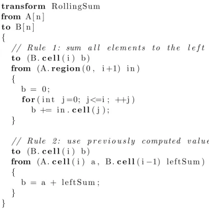
Figure 3.4 shows the data layouts in both nodes before and after a migration. During task migration, the task sender (Node 1) sends a metadata about RegionMatrix to the receiver (Node 2) along with the task migration message. This metadata contains information to dereference coordinates, and a reference to the original data on the sender. The receiver will create a new
Node 1
RegionHandler
RegionData RegionMatrix
(a) Before data migration.
RegionMatrixProxy RegionHandler RegionData RegionMatrix RegionHandler RegionDataRemote Node 1 Node 2
(b) After data migration.
Figure 3.4: Data migration process.
RegionMatrix from this metadata, as well as a RegionHandler and a RegionDataRemote. Then, a RegionDataRemote sends a request to the task sender to create a new RegionMatrixProxy pointing to the original RegionHandler. After that, the receiver can access data using RegionMatrixProxy in the sender.
We use a host identifier (HostPid) and a local pointer to original RegionHandler (Node 1) to identify the target handler. For each node, we also keep per-HostPid maps for all remote RegionHandlers that maps a remote pointer to a local RegionHandler. In Figure 3.5, after the migration, a new RegionMatrix shares the same RegionHandler with the former one. As a result, later accesses to the same RegionHandler do not need to establish a RemoteObject pair again.
RegionMatrix Proxy RegionHandler RegionData RegionMatrix RegionHandler RegionDataRemote Node 1 Node 2 RegionMatrix
(a) Before data migration.
RegionMatrix Proxy RegionHandler RegionData RegionMatrix RegionHandler RegionDataRemote Node 1 Node 2 RegionMatrix
(b) After data migration.
Figure 3.5: Data migration process when a RegionMatrix shares a RegionHandler with another RegionMatrix.
Note that this map is in RegionHandler level, which means multiple sub-matrices can share the same RegionHandler for remote data access. This reduces a number of RemoteObject pairs in the system. It also helps with data cache since multiple RegionMatrices access remote data using the same RegionHandler and RegionDataRemote. We will discuss about data cache in Section 3.7.
In some cases, we might have a long reference chain. For example, we migrate data from Node 1 to Node 2, and from Node 2 to Node3. As a result, Node 3 needs to send a request to Node 2, which forwards a request to Node 1. In order to eliminate excessive communications, RegionHandler has a method to update this reference chain by replacing RegionDataRemote with a new one that point
to data owner, or with a RegionDataRaw if data is local. We can also pass an information about RegionHandler in the owner node during task migration so that we do not create a long reference chain. Currently, this approach works since we know data location at the creation time, and do not move data after that.
3.4
Clone RegionDataSplit
RegionDataRemote RegionDataSplit
Node 1 Node 2
RegionDataRemote RegionDataRaw
Node 3
(a) Before cloning RegionDataSplit.
RegionDataSplit
Node 1 Node 2 Node 3
(b) After cloning RegionDataSplit.
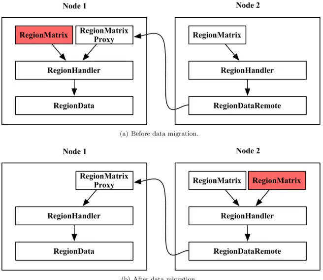
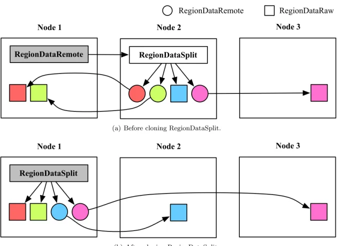
Figure 3.6: Cloning RegionDataSplit process.
Accessing a remote RegionDataSplit can be costly. For instance, in order to access the red part from Node 1 in Figure 3.6(a), we need to pass the request to Node 2, which forwards the request back to Node 1. We could optimize accessing a remote RegionDataSplit by cloning it to the local memory. By having a local RegionDataSplit, we can also query which nodes have data for a specific sub-matrix without sending any remote messages. Moreover, in localCopy and
fromScratchRegion (Section 3.5.2), we can directly fetch data from the data owner without passing the request through the original RegionDataSplit.
During the data migration, we pass a flag indicating whether the data is a RegionDataSplit. As shown in Figure 3.6, before accessing the data on Node 1, we clone the RegionDataSplit from Node 2. For each part, Node 1 creates either a new RegionDataRemote to directly connect to the data owner, or a pointer to the local data if the part is local. Hence, we can access parts with fewer network hops. Finally, we atomically replace a reference to the original RegionDataRemote in RegionHandler on Node 1 with a reference to the new RegionDataSplit.
3.5
Data Access
Programmers access data using cell method; for example, A.cell(0,0). In a shared memory version, cell returns a reference to an element (ElementT&). However, in a distributed version, the data can be remote, so a standard reference does not work. Hence, we create a proxy object for cell access. Furthermore, since accessing remote data cell-by-cell incurs a lot of network roundtrip costs, RegionMatrix supports copying sub-matrix to local memory for faster access.
3.5.1 Cell
In a distributed version, cell() returns a CellProxy object. CellProxy is a reference to a cell of a RegionData, which can be remote. It simulates a conventional reference to an address in the local memory. CellProxy has a pointer to a RegionHandler and a coordinate of the element in the referenced RegionData. CellProxy access is expensive, even though the data is local, because we need to allocate a new object, and pass multiple indirections in order to access the data. This is one of the major costs of using distributed data.
We overload various operators in CellProxy to simulate a reference to an element. Thus, we can generate a distributed version of PetaBricks programs without modifying the existing sources. Ternary operator is the only exception. It requires both result values to be the same type, and does not support implicit type casting. As a result, we have to explicitly cast the value in PetaBricks source codes. For example, we need to change
ElementT result = flag ? 0 : A.cell(0,0);
to
ElementT result = flag ? 0 : (ElementT) A.cell(0,0);
3.5.2 Sub-Matrix
Although programmers access data using cell method, we can optimize the data transfer by using sub-matrix accesses. The compiler can analyze the program and identify all data that each rule accesses. Thus, we can fetch the entire sub-matrix before applying the rule (see Section 4.3).
RegionMatrix provides 2 methods for sub-matrix access:
void localCopy(RegionMatrix& scratch, bool cacheable); void fromScratchRegion(const RegionMatrix& scratch);
The compiler uses localCopy and fromScratchRegion to copy remote data to a local scratch matrix, and copy it back after the modifications. A scratch matrix must have the same size as the source matrix, and must have a RegionDataRaw in a storage layer. Furthermore, this RegionDataRaw must have the same size as the source matrix as well. localCopy will populate a scratch matrix with data from the source. We begin this process by passing a metadata about the source matrix to the data owner. The data owner will reconstruct a requested sub-matrix, copy it to local storage, and send this storage back. fromScratchRegion is essentially an inverse of localCopy.
In the case where the original RegionMatrix is local (RegionDataRaw). Instead of creating a copy of storage, localCopy will copy all metadata of the original to scratch, and update scratch’s RegionHandler to the original RegionHandler. Thus, any modifications to the scratch will be seen by the original. Consequently, fromScratchRegion does not need to copy any data back to the original when the original matrix is local.
If the original RegionMatrix has a RegionDataSplit, we forward the request to affected parts, and construct a new metadata for each of them. In a special case where there is exactly one affected part, and the part is local, we will use the existing RegionData (a part of RegionDataSplit) instead
of creating a new one during localCopy. fromScratchRegion does not need to do anything other than changing pointers if the scratch RegionData is the same as the part RegionData.
3.6
Convert to Shared Memory Representation
The distributed data representation incurs overhead such as
1. Multiple indirections and virtual method invocations from RegionMatrix to RegionData.
2. Allocation of CellProxy objects for cell accesses.
3. Remote data fetches for accessing remote matrices.
For faster data accesses, we can convert RegionMatrix to a shared memory version so that we do not have this overhead. Since PetaBricks has a unified interface to manage data across all memory hierarchy, the C++ code to access distributed data is the same as the one for shared memory data. Thus, we can switch to a shared memory version without any code modifications.
When the matrix is local (RegionDataRaw), we can convert RegionMatrix to a shared mem-ory version by just converting metadata from a distributed version to a shared memmem-ory version. Specifically, we convert the metadata from split/slice information to base and multipliers. Since RegionDataRaw uses the same data storage as a shared memory matrix (see Section 3.1.3), the shared memory version can share the same storage object with the original RegionMatrix. As a result, both matrices will see changes in either of them.
When the matrix is remote or split, we use localCopy (in Section 3.5.2) to copy data from remote nodes to local memory. Then, we can convert the copy to a shared memory version. If there are any data modifications, we have to copy the local sub-matrix (distributed version) back to the original RegionMatrix.
3.7
Data Consistency
PetaBricks distributed data does not have sequential consistency guarantees. It supports multiple readers and writers without locks. Programmers have to explicitly identify all data required for
the computation, and all modified data. The compiler uses this information to generate a task dependency to ensure that there is no data race while using localcopy. As a result, the data layer does not need to support any consistency primitives. We will explain how the compiler does this in Section 4.3 and 4.4.
Nonetheless, we use cache for some remote data accesses. There are 2 access patterns, so we uses 2 different approaches to manage cache consistency. In general, the data layer provides a method to invalidate cache, and the runtime calls this method when the cache may be stale. We use the task dependency graph to invalidate the cache.
3.7.1 Cell Cache
The goal for this cache is to improve the speed of iterating over a small sub-matrix. Thus, we need a fast cache implementation. In addition, this type of iterations usually occurs at the leaf of the recursive decomposition process, where all accesses are originated from a single thread. Hence, we could use a thread-local cache to eliminate the need of locks.
We use a direct-mapped cache for cell accesses via RegionDataRemote. We implement this in a per-worker-thread basis in order to get a lock-free cache. Each read request will fetch a chunk of data together with start and end to indicate valid elements within the cache line because a part of RegionDataSplit might not have the entire cache line. Subsequent requests will try to get data from cache before sending a request to a remote node.
For cell writes, we modify the cache, and send a request to update the original matrix. We cannot wait and send updates at the eviction time because another thread might modify data in the same cache line. Although the changes do not affect the computation of the current thread, we cannot replace the entire cache line in the original matrix with the one from the current thread without the risk of placing stale data.
At the beginning of each task, we invalidate the cache by destructing the cache map to flush all cache in the worker thread. Since the consistency is guaranteed by a task dependency graph, there will be no data race within a task. However, we cannot take advantage of temporal locality because we frequently invalidate the cache.
In most cases, we do not use this cache. It relies on a spatial locality; however, PetaBricks can compute an applicable region for each rule. Consequently, we can prefetch data, using sub-matrix accesses, and access cells from a local copy of RegionMatrix instead of the original remote one.
3.7.2 Sub-Matrix Cache
The goal for this cache is to reduce the data transfer in the network. Multiple tasks on the same node might require the same piece of data, so we could fetch the sub-matrix once and cache it locally. It is acceptable for this cache to be slow since fetching a large packet over the network is very slow. Thus, we decide to have all threads shared the same cache.
We cache sub-matrix accesses in RegionHandler layer, and allow multiple threads to access the same cache. We need to use a lock to protect the cache. However, as opposed to cell cache, we infrequently use localCopy. Hence, even though we need to grab a lock before accessing the cache, there will be a low rate of lock contention.
Each RegionHandler maintains a map from a metadata of a sub-matrix to a RegionHandler for that sub-matrix. If a metadata matches an item in the cache, localCopy will change scratch’s RegionHandler to the one in the cache. Since RegionDataRaw of scratch has the same size as the source matrix, we do not need to modify a metadata of the scratch RegionMatrix.
All writes go directly to the RegionHandler, so the cache layer does not have to support cell writes. However, we need to purge stale data. Since the cache is shared by all threads in the node, we only need to invalidate cache when we have a cross-node task dependency. This can occur during 2 events:
1. Receiving a remote task, and
2. Receiving a remote task completion message.
A task might have some data dependency from nodes other than the sender, so we invalidate all cache on the receiver. Nonetheless, since a good schedule infrequently schedules remote tasks, we can expect to get a high cache hit rate.
As opposed to cache for cell access where all cache items are stored at the same place, sub-matrix cache items are in several RegionHandlers. Thus, we use a version number to invalidate
cache. Each node has its own version number, and each cache item also has a version number. Cache is valid when the version numbers match. Whenever we want to invalidate cache on any node, we increment its version number
Chapter 4
Distributed Scheduler
PetaBricks dynamic scheduler is completely distributed. To ensure the consistency, we use a task dependency graph to manage computation order. The existing work-stealing scheduler already implements this task dependency chain. As a result, we choose to extend it to a distributed version, which supports task migrations across machine boundaries. Furthermore, to improve data locality, the scheduler migrates tasks to nodes that have the most data required to apply the task. Since accessing distributed data is slow, we generate multiple versions of codes for different type of data, and switch to a faster version when possible. This allow us to eliminate all overhead to access remote data and schedule remote tasks.
PetaBricks compiler generates multiple versions of code: distributed, work-stealing, and sequen-tial. Distributed code can spawn tasks across multiple nodes. It uses a distributed data layer as described in Chapter 3. As a result, it incurs a high data access and scheduling cost. Work-stealing code can spawn tasks for a work-stealing runtime in the same node. It uses a shared memory data layer, which it can directly access cells in the local memory. Sequential code does not spawn any tasks. Nonetheless, it can still do recursive blocking to improve cache performance. Hence, it is the fastest version.
PetaBricks starts running in a distributed version of code, and allocates input data as specified in a configuration file. The scheduler will either enqueue a task in the local work-stealing queue, or migrate it to another node based on data location. This will eventually spawn tasks to all nodes
Node 2 Node 3
Node 1 Node 4
Distributed Work-stealing Sequential
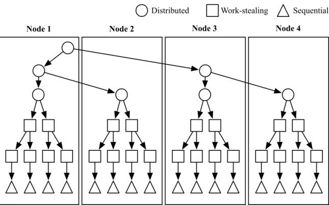
Figure 4.1: Overview of PetaBricks distributed runtime.
in the system. During the execution of each task, PetaBricks can choose to spawn a work-stealing task instead of a distributed version. After that, a work-stealing task can choose to call a sequential code. We cannot go in the backward direction. For example, a work-stealing task cannot spawn a distributed task. Figure 4.1 illustrates this process. The general idea is to distribute tasks across all nodes in the very beginning, and run a work-stealing schedule on each node after the initial migration.
Apart from worker threads, each node has a few dedicated listen threads to process incoming messages from other nodes. They process data-related messages such as data creation and data access. They also process task-related messages such as task migration and task completion. Al-though worker threads can help processing messages, the listen thread is the primary component for incoming communication.
Section 4.1 outlines the migration process. Section 4.2 specifies the place where we can migrate tasks. Section 4.3 describes an optimization to prefetch data to local memory for faster remote data access. Section 4.4 explains how we convert to a work-stealing schedule in order to eliminate
the distributed overhead. Finally, Section 4.5 describes the distribution of data.
4.1
Task Migration Process
We extend the work-stealing scheduler in the shared memory version of PetaBricks to support a distributed memory model. To improve data locality, we decide to dynamically schedule distributed tasks using data locations instead of using a work-stealing approach.
The complication of the distributed task migration are references to matrices. In a shared memory system, we can pass a pointer to a matrix in the heap to other workers because all workers share the same address space. In the distributed version, we have to migrate RegionMatrices along with the task. Another issue is to notify the task sender after the completion to enable the other tasks that depend on the completed one.
In the work-stealing runtime, the unit of computation is a DynamicTask, which stores a call frame in the heap instead of the stack so that the task can be migrated between processors in the same machine. For the distributed version, we use a RemoteTask, which is a subclass of DynamicTask that does the following:
1. scheduling tasks across multiple nodes,
2. serializing tasks,
3. unserializing tasks,
4. managing remote task dependency.
First, the task, which could be scheduled on another node, must be a RemoteTask. When the task is ready to run, we will query the location of all data that is needed by the task. Then, schedule the task on the node with the most data. If the target is localhost, we just put the task in the local work-stealing queue. If the target is remote, we continue to the second step.
Second, we serialize the task and send it to the target. Since the task contains all information it needs to run, we do not have to worry about memory on the stack. However, the task might
have pointers to matrices in the local memory, which remote workers could not access. Thus, we need to migrate these matrices along with the task, as described in Section 3.3.
Third, a task receiver unserializes the task, and completes all data migrations. Then, it puts the task in its local work-stealing queue so that worker threads can run the task.
Finally, a task receiver must notify the sender when it finishes running the task. The receiver does this by creating a task to notify the sender about the completion. Then, it makes this new task depended on the received task so that it gets run after the received task completes. After the sender receives the notification, it enqueues all tasks that depend on the completed task.
Apart from a migration overhead, RemoteTask also has a high scheduling overhead in the first step. Although it eventually enqueues a task locally, it needs to figure out the location of all matrices, which can be very slow when there are a lot of data. Hence, we choose to create a DynamicTask instead of a RemoteTask when we do not want to migrate the task.
4.2
Migratable Tasks
We choose to migrate tasks that could take a long time to complete; otherwise, we will end up spend a lot of time migrating tasks. For each type of migratable tasks, we need to compute the applicable region for each referenced data in order to determine where to enqueue the task.
There are 2 types of tasks that can be migrated to remote nodes: cross transform and during recursive decomposition.
4.2.1 Cross Transform
We can migrate a task when we call another transform. For example, in Figure 4.2, Mergesort calls SORT and Merge. The first SORT will be migrated to where the most of the first half of tmp and in is. Similarly, we could migrate the second SORT and Merge to other nodes.
We implement this by making a distributed version of a transform task be a subclass of Re-moteTask. As a result, whenever we enqueue the task, the scheduler will check the location of data and migrate the transform to where most data live. In this case, the applicable regions are the entire to-matrices and from-matrices of the transform.
transform M e r g e s o r t from IN [ n ] to OUT[ n ] { to (OUT o u t ) from ( IN i n ) using ( tmp [ n ] ) { i f ( n > 1 ) {
spawn SORT( tmp . region ( 0 , n / 2 ) , i n . region ( 0 , n / 2 ) ) ; spawn SORT( tmp . region ( n / 2 , n ) , i n . region ( n / 2 , n ) ) ; sync ;
Merge ( out , tmp . region ( 0 , n / 2 ) , tmp . region ( n / 2 , n ) ) ; } e l s e {
o u t . c e l l ( 0 ) = i n . c e l l ( 0 ) ; }
} }
Figure 4.2: PetaBricks source code for Mergesort
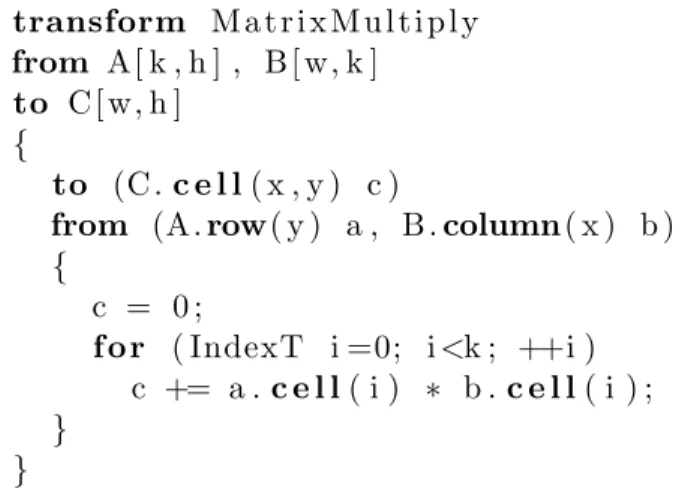
4.2.2 During Recursive Decomposition
transform M a t r i x M u l t i p l y from A[ k , h ] , B [ w, k ] to C [ w, h ]
{
to (C . c e l l ( x , y ) c )
from (A. row( y ) a , B . column ( x ) b ) { c = 0 ; f o r ( IndexT i =0; i <k ; ++i ) c += a . c e l l ( i ) ∗ b . c e l l ( i ) ; } }
Figure 4.3: PetaBricks source code for MatrixMultiply
We can also migrate tasks during a recursive decomposition process. For example, Matrix-Multiply, in Figure 4.3, does not call any transform, but we can decompose the computation into multiple tasks based on the coordinates of matrix C, as shown in Figure 4.4. We call the new task a SpatialMethodCallTask. Each SpatialMethodCallTask applies the same rule for
differ-ent regions of C, and could be migrate to another node. We can also recursively decompose a SpatialMethodCallTask into smaller tasks.
w h w/2 h/2
C
Applicable Regions A BFigure 4.4: Decomposing the computation of the rule in MatrixMultiply based on C
We have multiple versions of SpatialMethodCallTask for the work-stealing scheduler and the distributed scheduler. The one for the distributed scheduler is a subclass of RemoteTask. We compute the applicable regions for each iteration space, and migrate the task to the node that contains the most data in the applicable regions. Figure 4.4 shows the applicable regions of A and B for the task that applies for the top-left region of C.
Since computing applicable regions and querying data location take a lot of time, we try to reduce the number of distributed SpatialMethodCallTasks. Thus, we switch to the work-stealing version of SpatialMethodCallTask when we do not want to migrate data.
4.3
Prefetch Remote Data
In order to speed up the remote data access time, we can prefetch data from remote nodes to local memory, using sub-matrix access methods in Section 3.5.2. As a result, subsequent data accesses do not require any remote fetches. However, we still have the overhead for accessing distributed data, which we will address in Section 4.4.
In order to get a good performance from prefetching, we have to be very careful to prefetch only necessary values. For correctness, we also need to make sure that the prefetch values are up-to-date, and that all modified values are written back to the original place.
We do this optimization at the leaf of the recursive decomposition, where we prefetch all ap-plicable regions. For example, in MatrixMultiply, when computing the top-left of C , we prefetch the top-left of C and applicable regions of A and B (grey parts in Figure 4.4) to scratch matrices. Then, we use the scratch matrices during the computation of the leaf. Finally, we copy a part of C back to the original matrix. (In the MatrixMultiply case, we can do better than this. See Section 4.4.2.)
At the leaf iterations, we know which data is needed, so we will not fetch unnecessary data. Moreover, there is no external task dependency during the leaf iteration, so we do not have to invalidate the scratch during the iteration. However, the most important aspect of leaf iterations is that we know which data is modified. Since we need to write modified data back to the the original matrix at the end of the task, we must make sure that we do not overwrite the original data with stale data in scratch. The leaf iteration has this property because it writes to all elements in to-matrix by a language definition. Thus, we will not write stale data back to the original matrix.
4.4
Convert to Work-Stealing Schedule
Using the prefetching technique can reduce the number of remote fetches; however, there is still a high overhead for accessing data. Although the data is local, a distributed data layer requires at least three levels of indirection to get to the actual cell. Furthermore, using a distributed scheduler also incurs an overhead of querying data locations. Hence, we aggressively convert the computation
to a work-stealing schedule.
There are 3 main issues in switching to a work-stealing schedule.
1. We cannot create a distributed task after switching to a work-stealing schedule because it uses shared memory matrices.
2. We need to create local shared memory matrices for a work-stealing schedule. Since we may copy remote data to create them, we have to make sure that we use most of the copied data. We also need to update all indices to those of the new matrices.
3. Since we need to copy some data to a scratch matrix, we need to make sure that there is no data race during the work-stealing computation.
Similar to a task migration, we can convert to a work-stealing schedule during a cross transform, or during a recursive decomposition.
4.4.1 Cross Transform
When a task calls a new transform, we have a choice to call either a distributed version or a work-stealing version of the transform. If we choose a distributed version, we will continue to the task migration process. If we choose a work-stealing version, we will continue on a shared memory PetaBricks code. As a result, we can eliminate all overhead from distributed scheduling, and accessing distributed data.
In order to convert to a work-stealing transform, we need to convert all input and output matrices to a shared memory data representation. We do this by fetching all data to local memory, and creating a new metadata, as described in Section 3.6. Then, we pass these scratch matrices to a constructor of a transform task. Finally, we copy the outputs back to the original owners at the end of the transform.
Similar to prefetching during leaf iterations, there is no external task dependency during a transform. Consequently, we can prefetch the data at the beginning of the transform. In addition, every element in to-matrices must be written by the transform, so we can copy the entire to-matrices
back to remote nodes, without worrying about overwriting new data with the stale one. Hence, there will not be a data race.
In Mergesort example, we can run a work-stealing version of SORT and Mergesort. In order to use a work-stealing schedule for the first SORT, we need to copy the first half of tmp and in to local memory. At the end of SORT, we copy tmp back to the original place. It seems like we need to copy a lot of data; nonetheless, the scheduler will try to schedule the task so that the data is local. For instance, if the first half of tmp and in are in Node 1, and the rest is in Node 2. We will compute the first SORT in Node 1 and the second SORT in Node 2. Hence, in order to convert to a work-stealing schedule, we do not need to copy any data.
4.4.2 During Recursive Decomposition
We can also convert a distributed SpatialMethodCallTask to a non-distributed version, when we do not want to migrate a spatial task. There are 2 ways to do this, based on whether a leaf calls other transforms.
Use DynamicTask SpatialMethodCallTask
When a leaf calls other transforms, we do not want to run a work-stealing version of the leaf. Since a work-stealing code cannot spawn distributed tasks, a work-stealing version of the leaf cannot create a distributed instance of the transform. As a result, we decide to run a distributed version of the leaf. However, we can eliminate the scheduling overhead by using a DynamicTask version of a SpatialMethodCallTask.
Use Partial SpatialMethodCallTask
When a leaf does not call other transforms, we can run it in a work-stealing mode. Nonetheless, the leaf is a part of a rule, which is a part of a transform, so it shares matrices with the transform. If we naively convert all matrices to a shared memory representation, we will end up copying unnecessary data. Thus, we create a partial task that applies a part of a rule on shared memory data, and does not share matrices with a transform.
A partial task is similar to a recursive decomposition part of a work-stealing rule. It can spawn more partial tasks, and can call sequential codes. However, it uses references to matrices in a separate metadata instead of sharing them with a transform instance. Using a metadata allows a partial task to spawn more partial tasks without creating new matrices. This metadata contains references to shared memory matrices, and their offsets from the original distributed version. A partial task uses this information to compute indices of new matrices in the metadata.
During a recursive decomposition of a rule in MatrixMultiply, the scheduler can create a partial task, instead of a distributed SpatialMethodCallTask, to compute a part of C. It also create a metadata for the partial task by converting all applicable regions to shared memory matrices. The new partial task can spawn more partial tasks without creating a new metadata for child tasks. After all tasks are done, we copy modified data back to the original owners.
4.5
Data Distribution
Since the scheduler dynamically schedules tasks based on data location, in order to distribute the computation, we need to distribute data. We distribute data during the allocation of matrices. In a configuration file, we specify a data distribution for every input, output and temporary matrix, which is defined by the following keywords: to, from, through, and using. PetaBricks provides many ways to distribute data in each matrix.
1. Allocate Data Locally: The matrix will be allocated as a RegionDataRaw on the current node.
2. Allocate Data on One Remote Node: The matrix will be allocated as a RegionDataRaw on one of the remote nodes. The current node will access this matrix via a RegionDataRemote.
3. Allocate Data on Multiple Nodes: The matrix will be allocated as a RegionDataSplit on the current node, and each part of the matrix can be placed on different nodes. We can split the matrix by row, column or block into any number of equal parts.
Chapter 5
Auto-tuning Parameters
The compiler exposes the following parameters to the auto-tuner: distributed cutoff, and data distribution. We have to expose enough parameters to get a high performance, but not too many so that the auto-tuner can tune them. Nonetheless, we have not implemented the auto-tuner for these parameters in this thesis.
5.1
Distributed Cutoff
In Section 4.4, we convert a distributed schedule to a work-stealing schedule. The scheduler uses a distributed cutoff to determine which schedule it should use. Whenever the size of applicable data is smaller than a distributed cutoff, we switch to a work-stealing schedule. If a distributed cutoff is too big, we may not distribute computations to all nodes. If it is too small, there will be a high overhead of using distributed scheduler and data representation.
5.2
Data Distribution
In Section 4.5, a configuration file specifies how each matrix is distributed. For each matrix, we have 3 tunable parameters:
1. Distribution Type: We can either allocate matrix on a localhost, allocate matrix on a remote node, split matrix by row, split matrix by column, or split matrix by block.