HAL Id: hal-00317062
https://hal.archives-ouvertes.fr/hal-00317062
Submitted on 1 Jan 2003
HAL is a multi-disciplinary open access
archive for the deposit and dissemination of
sci-entific research documents, whether they are
pub-lished or not. The documents may come from
teaching and research institutions in France or
abroad, or from public or private research centers.
L’archive ouverte pluridisciplinaire HAL, est
destinée au dépôt et à la diffusion de documents
scientifiques de niveau recherche, publiés ou non,
émanant des établissements d’enseignement et de
recherche français ou étrangers, des laboratoires
publics ou privés.
activity
A. D. Danilov
To cite this version:
A. D. Danilov. Long-term trends of foF2 independent of geomagnetic activity. Annales Geophysicae,
European Geosciences Union, 2003, 21 (5), pp.1167-1176. �hal-00317062�
Annales Geophysicae (2003) 21: 1167–1176 c European Geosciences Union 2003
Annales
Geophysicae
Long-term trends of foF2 independent of geomagnetic activity
A. D. Danilov
Institute of Applied Geophysics, Rostokinskaya 9, Moscow 129 128, Russia
Received: 28 January 2002 – Revised: 28 August 2002 – Accepted: 25 October 2002
Abstract. A detailed analysis of the foF2 data at a series of
ionospheric stations is performed to reveal long-term trends independent of the long-term changes in geomagnetic ac-tivity during the recent decades (nongeomagnetic trends). The method developed by the author and published earlier is used. It is found that the results for 21 out of 23 stations con-sidered agree well and give a relative nongeomagnetic trend of −0.0012 per year (or an absolute nongeomagnetic trend of about −0.012 MHz per year) for the period between 1958 and the mid-nineties. The trends derived show no depen-dence on geomagnetic latitude or local time, a fact confirm-ing their independence of geomagnetic activity. The consid-eration of the earlier period (1948–1985) for a few stations for which the corresponding data are available provides sig-nificantly lower foF2 trends, the difference between the later and earlier periods being a factor of 1.6. This is a strong argument in favor of an anthropogenic nature of the trends derived.
Key words. Ionosphere (ionosphere-atmosphere
interac-tions; ionospheric disturbances; mid-latitude ionosphere)
1 Introduction
Studies of the long-term changes (trends) in the parameters of the upper atmosphere and ionosphere are currently very popular. Several groups of authors (Bencze et al., 1998; Bremer, 1996, 1998, 2001; Danilov and Mikhailov, 1998, 1999, 2001; Givishvily and Leshchenko, 1993, 1994; Jarvis et al., 1998; Marin et al., 2001; Mikhailov and Marin 2000, 2001; Ulich and Turunen, 1997; Ulich et al., 1997; Upad-hyay and Mahajan, 1998) studied trends of the F2-layer pa-rameters, hmF2 and foF2. The results of these studies dif-fer significantly, both by the methods of trend revealing used and the results obtained (see the recent review by Danilov, 2002a). The reason for such “popularity” of the searches for long-term trends of the F2-layer parameters is that the
ver-Correspondence to: A. D. Danilov (adanilov99@mail.ru)
tical sounding data used to derive these trends are the only ground-based data available for several decades, providing a possibility to find whether there are long-term trends in the upper atmosphere (in the thermosphere, in particular) of an anthropogenic origin similar to those found in the middle at-mosphere.
Danilov and Mikhailov (1998; 1999) were the first to at-tract attention to the fact that the trends of the critical fre-quency foF2 obtained at different stations demonstrate a de-pendence on the station geomagnetic latitude 8 decreasing with a decrease in 8. This was an important starting point for the concept that the trends found by the so-called rel-ative trend method (for details see Danilov, 2002a) are re-lated to the changes in geomagnetic activity during the recent decades.
Mikhailov and Marin (2000, 2001) and Marin et al. (2001) further developed this concept and claimed that the foF2 and
hmF2 trends manifest the long-term changes in geomagnetic
activity during the period of observations. The above authors demonstrated, in particular, that the foF2 trends obtained un-dergo diurnal variations and variations with the geomagnetic latitude, which indicate a relation between the Ap geomag-netic index and the foF2 trends.
However, Danilov (2002a, b) demonstrated that the long-term changes in the geomagnetic activity cannot alone be re-sponsible for the foF2 trends observed. For some time inter-vals (for details and examples see Danilov, 2002b) there are no systematic changes in Ap at all but significant trends of
foF2 are distinctly seen in the ionospheric data. This was the
starting point of the concept suggested by Danilov (2002b) according to which the foF2 trends found by the relative trend method and studied in detail by Danilov and Mikhailov (1999, 2000) and Mikhailov and Marin (2000, 2001) and Marin et al. (2001) are a combination of two effects: the geomagnetic trend caused by the long-term changes in geo-magnetic activity and a nongeogeo-magnetic trend (i.e. the trend independent of geomagnetic activity). The nature of the lat-ter trend is not finally clear, but there is a significant chance that if it exists, it is of an anthropogenic nature.
Danilov (2002b) developed a method to reveal nongeo-magnetic trends in foF2 against the background of the vari-ations of this parameter with geomagnetic activity and de-scribed in detail the work of the method using the data on
foF2 measured at the Sverdlovsk ionospheric station (ϕ =
56.7 N and 8 = 48.4 N). A summary of the trend determi-nation for the Irkutsk station (ϕ = 52.7 N and 8 = 41.1) was also presented. For both stations a significant nongeomag-netic trend (k(tr) = −0.00115 per year and −0.00128 per year, respectively) was found.
In this paper the method developed by Danilov (2002b) is applied to a set of ionospheric stations and the results ob-tained are analyzed in terms of the trend dependence on the geographic and geomagnetic coordinates, local time, and pe-riod of observation.
2 The method and data
Actually, Danilov (2002b) proposed two methods to de-rive the nongeomagnetic trend. It was demonstrated that both methods give almost the same results. This is why in this study we used only one of the methods (called in Danilov, 2002b as Method I). It is worth mentioning briefly the essence of the method.
The method is based on the assumption that the observed trend of foF2 k(obs) is a result of a linear combination of two different trends: the geomagnetic trend (i.e. the trend caused by the long-term changes in geomagnetic activity) and the nongeomagnetic trend k(t r). It is also assumed that the changes in geomagnetic activity are described by annual mean values of the Ap index and that the geomagnetic trend in foF2 (or hmF2) is proportional to the changes in Ap (to the gradient of Ap k(Ap)) for the period considered. In such a case we have a very simple formula for k(t r):
k(tr) = k(obs) + a1k(Ap). (1)
To describe the Ap changes in each 30-year interval we used the coefficient k(Ap) of the Ap linear regression within the interval considered: Ap(X) = Ap(X1)+k(Ap)(X−X1),
where X1is the first year of the interval in question and X is
the current year. Actually, k(Ap) is merely the slope of the linear approximation of the Ap value plotted versus the years of the given interval.
The coefficient a1 is, first of all, a scaling coefficient,
which takes into account different values in which k(obs) and k(Ap)are obtained due to the difference in absolute values of δfoF2 (the difference between the observed and model values
of foF2 in relative units used in the relative trend method as a main parameter temporal changes of which are analyzed) and Ap. However, it was assumed by Danilov (2002b) that the a1coefficient also includes the efficiency of the magnetic
activity impact on foF2 and so it might change with local time and from one station to another. The data described in this paper confirm this assumption completely.
There is no way to measure or evaluate the a1coefficient
directly. Danilov (2002b) proposed the following method
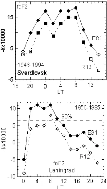
Fig. 1. Relative trends of foF2 for the Sverdlovsk (top) and Leningrad (bottom) stations derived using the R12 and E81 indices. The closed and open symbols in the top panel correspond to the sta-tistical significance above and below 90% according to the Fisher criterion. The horizontal line in the bottom panel shows approx-imately the k value for the significance of 90% according to the Fisher criterion.
of a1 determination. The entire time interval studied (for
example, 1948–1994 for the Sverdlovsk station in Danilov, 2002b) is split into running 30-year intervals (1948–1987, 1949–1988,..., and 1965–1994). The foF2 trend value k(t r) is found for each interval with various values of a1. The
re-quirement is superimposed so that there should be no corre-lation of the values k(t r) obtained for each 30-year interval and k(Ap) values for the same interval. This requirement is very simple and follows from the essence of the nongeomag-netic (independent on geomagnongeomag-netic activity, i.e. on k(Ap)) trend we are looking for. However, this requirement makes it possible to find the a1coefficient unambiguously. To make
A. D. Danilov: Long-term trends of foF2 independent of geomagnetic activity 1169 of the correlation coefficient r[k(tr), k(Ap)] between k(tr)
found and k(Ap) over all the 30-year intervals should be less than 0.1. Actually, the computer program (see below) was looking for a minimum in the r[k(tr), k(Ap)] value, so in the real calculations considered in this paper the value of r[k(t r), k(Ap)]in the majority of cases was much less that 0.01 and very often was close to 0.001 (see tables below).
The values of k(tr) obtained for each 30-year interval were then averaged over all the 30-year intervals and this provided a k(t r, ave1) value for the particular moment of LT. The pro-cedure was performed for every even LT hour for every sta-tion.
A computer program was developed to perform the anal-ysis described above and to find k(tr, ave1) values. The input data were the initial ionospheric data, the 12-month smoothed E81 index, and the annual mean Ap values. As an output the program provided k(t r, ave1), its standard de-viation σ due to the averaging of k(tr) over all the 30-year intervals, the a1coefficient and the minimum modulus of the
r[k(t r), k(Ap)]value it succeeded to reach.
To apply the method to a big set of data, we took the data of 23 ionospheric stations of the western hemisphere. The data were collected from different sources, including CDs, Inter-net, World Data Center B in Moscow, and the Geophysical Databank collected in the Moscow ISES Warning Center.
The first requirement of the data was very simple: there should be not less than 30 + 5 years of permanent observa-tions. The 30-year length and the number 5 represent the shortest interval length and the least number of 30-year in-tervals for which the procedure described is stable and pro-vides reliable results. These values were found empirically by playing with the program. It is worth noting that only for one station chosen (Mundaring, see below Table 3) there were 5 intervals and for one station (Dikson) there were 6 in-tervals. For the majority of the stations considered the above number was 8–10.
The second requirement was that the time interval of data available should last at least to the beginning of the 1990s (to 1991). Again, the data for only one station (Irkutsk) stopped too early. For one more station (Dikson) the data stopped in 1992. The majority of the stations covered a significant part of the 1990s (see below Table 3).
Many ionospheric stations were opened and started regular operation during the International Geophysical Year, so data for them are available after 1957. Since in the process of 12-month smoothing we lose one year in the beginning and at the end of any data set, the analyzed period for many stations started in 1958. This is why for the main analysis we took for all stations the period from 1958 to the end of the available data. The stations Tashkent (the analyzed interval begins in 1962), Mundaring (1960), Ashkhabad (1959) present excep-tions (see Table 3), since they started operaexcep-tions a few years later. For the Irkutsk station the entire period of observation was taken, so the analyzed period was 1949–1991. The sta-tions for which there are data for a considerable period before 1958 will be particularly considered below.
Contrary to the papers dedicated to relative trend determi-nation (Danilov and Mikhailov, 1999; Mikhailov and Marin, 2000, 2001), in this paper we used as a solar activity index not the sunspot number R12, but the index E81 proposed and provided by Tobiska et al. (2000). This index is much more closely related to the solar UV radiation forming the F2-layer, so one may expect this index to be better for get-ting rid of the changes induced by solar activity variations. To have the same smoothing for both foF2 and solar index data we used a 12-month smoothing of the E81 index.
Figs. 1 and 2 demonstrate that it is actually so. Figure 1 shows the relative trends (without getting rid of the geo-magnetic activity effects) of the same type as considered by Danilov and Mikhailov (1999, 2001) and Mikhailov and Marin (2000, 2001), calculated using the R12 and E81 in-dices. One can see that for both stations and for all LT mo-ments the trends derived with the help of E81 are slightly but systematically higher than the trends based on R12. The difference may not look very large but it influences the statis-tical significance of the trends derived. For example, for the Leningrad station five points for E81 are above the 90% sig-nificance level by the Fisher criterion, whereas for R12 there is only one such point.
Figure 2 provides a similar example. This time the trends themselves are the same if R12 or E81 is used, but the cor-relation coefficient squared (which determines the statistical significance by the Fisher criterion if the number of points is fixed) is considerably higher for E81 than for R12.
The above considerations determined the choice of the E81 index as a solar activity index in the calculations de-scribed in this paper. This choice has one small disadvantage: there are data for the E81 index only since 1948. For the re-sults presented below it is sufficient. However, if the data for this index for much earlier years existed, one could try to an-alyze in the way described here the data of the Slough station since the 1930s.
Thus, the initial data for the calculations of nongeomag-netic trends were 12-month running mean values of foF2 and the E81 index. Due to the essence of the method, all years within any chosen 30-year interval were used and no attempts were made to use only the years of solar maxima and minima, as it has been done in many papers dealing with the relative trend method.
3 Calculations
After the calculation of the k(t r, ave1) values for the given station for each particular moment of LT, a table was com-piled. Typical examples of this table for a high-latitude sta-tion (Kiruna) and a mid-latitude stasta-tion (Tashkent) are pre-sented in Tables 1 and 2. Such tables were compiled for every station and they were the main material for check-ing the computcheck-ing program operation and derivcheck-ing a final value of the nongeomagnetic trend k(t r, ave2) for the par-ticular station. Each table contains: local time, the corre-lation coefficient r(δf oF2, Ap), the correcorre-lation coefficient
Fig. 2. Relative trends of foF2 for the Moscow station (top) and the
correlation coefficient squared (bottom panel) for the data of the top panel. Only the years around maxima and minima of solar activity since 1965 were used (see Danilov and Mikhailov, 1999).
r[k(obs), k(Ap)], the a1 coefficient, the correlation
coeffi-cient r[k(t r), k(Ap)], the trend value k(tr, ave1) and the standard deviation σ (1). The column “accepted” shows the values of k(t r, ave1) accepted for the averaging over LT and obtaining a final value of k(tr, ave2) for the given station.
The correlation coefficient r(δf oF2, Ap) shows the cor-relation between the deviations of foF2 from the regres-sion model (in terms of solar activity index, for details see Danilov and Mikhailov, 1999) δfoF2, and the Ap index. The stronger the geomagnetic influence on foF2 for this particular station and LT moment is, the higher the modulus would be of r(δf oF2, Ap). It is evident that it is easier to get rid of the geomagnetic activity effect in the k(obs) when the relation between foF2 and Ap is well pronounced. This is why, as a rule, the most stable picture is observed when r(δf oF2, Ap) is above 0.4. When r(δf oF2, Ap) is low, very often the pic-ture is unstable and the trend obtained for the particular LT is less than the standard deviation. It is worth remembering
that the k(t r, ave1) value for each LT moment is a result of the averaging over all the 30-year intervals used (available) for this particular station. If the geomagnetic effect is weakly pronounced, it has not been removed properly and the k(t r) values for each 30-year interval show strong scatter which is manifested in high values of σ (1).
All the above-said is illustrated by Table 1. We see that for LT = 22, 00, 02, 04, and 06 hours the modulus of r(δf oF2, Ap)is small and the corresponding values of k(t r, ave1) are less than σ (1). This fact is indicated in the last column of Ta-ble 1 and explains why the k(t r) values for the LT moments indicated were not included in the calculation of the final av-erage value of the trend k(t r, ave2) shown at the bottom of the table.
Therefore, as a first criterion for accepting or rejecting the k(t r, ave1) values obtained for each particular LT mo-ment we used the criterion that the modulus of r(δf oF2, Ap) should not be less than 0.1. The value is slightly arbitrary and is based only on the numerous “plays” with the tables similar to Tables 1 and 2. If this criterion is broken, it is shown in the Comments column as r < 0.1 (see Table 2, 00:00 LT).
The “trend < σ ” situation mentioned above is the second out of the three criteria. The third criterion is that the sign of the r(δf oF2, Ap) for every 30-year interval considered should be the same. If the sign changes during the entire period considered (for example, it is positive for the 1958– 1987, 1959–1988 intervals and is negative for the 1965– 1994, 1966–1995 intervals, or vice versa) the picture is un-stable and the corresponding trend is not accepted and this fact is indicated as “plus/min” in the Comments column. As a rule, the “plus/min” situation is accompanied by invalidat-ing other criteria for acceptinvalidat-ing k(t r, ave1) for this particular hour (in Table 1 for 00:00 LT all three criteria are not valid). It should be especially emphasized that if one of the above three criterion is not valid, it does not mean that the k(t r,ave1) for this particular LT moment is necessarily close
to zero or very small. It merely means that for this particular hour the initial data were not good enough for the method described to be used and so the scatter of the k(t r) obtained is large or the correlation between δfoF2 and Ap is low, the latter fact making it difficult to get rid of the geomagnetic ef-fect. “The data were not good” means that for one or a few years the monthly mean values for this particular LT initially used differ significantly from the values for the other LT.
One can see from Tables 1 and 2 that k(t r, ave1) val-ues acceptable for further averaging are not always obtained for all 12:00 LT moments considered because of the crite-ria for the acceptance described above. In particular, for the Kiruna and Tashkent stations (Tables 1 and 2) only 7 and 10 k(t r, ave1) values, respectively, are accepted and used to derive k(t r, ave2) for these stations. Only for 5 stations were all 12 k(t r, ave1) values accepted, with the least number of the values being 7 (Kiruna, Rome, and Irkutsk).
The analysis of the tables similar to Tables 1 and 2 shows that the signs of the a1 coefficient and r[k(obs), k(Ap)]
are always opposite without a single exception. It follows from the essence of the method, so this fact was used to
A. D. Danilov: Long-term trends of foF2 independent of geomagnetic activity 1171
Table 1. Calculation of the trends for the Kiruna station
LT A B a1 C k(t r,ave1) σ(1) accepted comments
0 −0.03 0.18 -0.0036 0.001 −0.00001 0.00191 plus/min 2 0.03 0.11 −0.0018 0.003 0.00068 0.00150 t r < σ 4 −0.05 0.17 −0.0024 0.001 0.00034 0.00130 t r < σ 6 −0.25 0.08 −0.0009 0.004 0.00046 0.00110 t r < σ 8 −0.44 −0.26 0.0022 −0.005 −0.00149 0.00078 −0.00149 10 −0.56 −0.4 0.0031 −0.003 −0.00155 0.00068 −0.00155 12 −0.53 −0.37 0.0029 −0.006 −0.0015 0.00070 −0.00150 14 −0.53 −0.49 0.0037 0.006 −0.00108 0.00062 −0.00108 16 −0.58 −0.53 0.0043 −0.004 −0.00148 0.00065 −0.00148 18 −0.58 −0.64 0.0045 −0.004 −0.00163 0.00051 −0.00163 20 −0.25 −0.18 0.0014 −0.001 −0.00094 0.00074 −0.00094 22 −0.17 0.09 −0.0012 0.001 −0.00047 0.00120 tr< σ R2= −0.96; R1= −0.98; k(tr, ave2) = −0.00138 per year; σ (2) = 0.00026
A = r(δf oF2,Ap); B = r[k(obs), k(Ap)]; C = r[k(tr), k(Ap)]
Table 2. Calculation of the trends for the Tashkent station
LT A B a1 C k(t r,ave1) σ(1) accepted comments
0 0.01 0.86 −0.0050 0.007 −0.00171 0.00025 r <0.1 2 −0.11 0.79 −0.0031 −0.011 −0.00170 0.00026 −0.00170 4 −0.22 -0.18 0.0004 −0.014 −0.00071 0.00020 −0.00071 6 −0.42 0.42 −0.0013 −0.009 −0.00129 0.00024 −0.00129 08 −0.14 0.90 −0.0018 −0.059 −0.00089 0.00069 −0.00089 10 0.17 0.92 −0.0029 0.010 −0.00073 0.00010 plus/min 12 0.25 0.82 −0.0023 −0.010 −0.00063 0.00014 −0.00063 14 0.24 0.71 −0.0017 0.017 −0.00068 0.00014 −0.00068 16 0.23 0.42 −0.0016 0.011 −0.00059 0.00011 −0.00059 18 0.26 0.93 −0.0027 −0.043 −0.00103 0.00009 −0.00103 20 0.16 0.95 −0.0061 0.022 −0.00145 0.00016 −0.00145 22 0.09 0.91 −0.0055 0.012 −0.00125 0.00210 plus/min R2=−0.33; R1=−0.73; k(tr, ave2) = −0.00100 per year; σ (2) = 0.00040;
A, B, and C denote the same as in Table 1
check the results of the k(tr, ave1) calculations by the pro-gram. There should be a negative correlation between a1and
r[k(obs), k(Ap)]. In an ideal case (if there were no scatter of the initial foF2 data) the correlation coefficient R1 between these two values would be equal to unity. However, in real-ity, it lies within the minus 0.70–0.99 interval, with the vast majority of the values of R1 being below −0.9. The values of the R1 coefficient for the Kiruna and Tashkent stations are shown at the bottom of Tables 1 and 2, respectively.
The second coefficient shown at the bottom of Tables 1 and 2 is the correlation coefficient R2 between a1and r(δf oF2,
Ap). On the average, it is of about minus 0.6–0.8, with a few values below minus 0.9 and the least absolute value −0.33 shown for the Tashkent station in Table 2. One should not expect a very high value of R2, because a1includes a
scal-ing factor (see above) which may change independently of the relation between δfoF2 and Ap. However, for all the sta-tions considered (except four) the fact that the values of R2
are statistically significant at the 95% level according to the Fisher criterion, they have the same sign (minus), and for some stations (Kiruna, Salekhard, Moscow) they are below −0.95, demonstrates that a1 also includes the degree of the
relation between δfoF2 and Ap. This is exactly what was assumed by Danilov (2002b) on the basis of the Sverdlovsk station analysis.
All the coefficients were used to check the computation results and to analyze the trends obtained. They also help in understanding how the method works and what is hap-pening at each particular station. The consistence of the re-sults obtained for the various stations (the same sign of the k(t r,ave2) trend, the high negative value of R1, and the
neg-ative values of R2 for all stations) is a confirmation of a cor-rectness of the method providing trends independent of geo-magnetic activity.
Table 3. The trends finally accepted for various stations
Station 8 ϕ λ k(t r,ave2) σ(2) years Dikson 63.1 73.5 80.4 −0.00138 0.00053 1958–1992 Loparskaya 63.4 68.0 33.0 −0.00127 0.00053 1958–1993 Kiruna 65.2 67.8 20.4 −0.00138 0.00026 1958–1997 Sodankyla 63.7 67.4 26.6 −0.00340 0.00090 1958–1997 Salekhard 57.3 66.5 66.7 −0.00127 0.00038 1958–1997 Lycksele 62.7 64.7 18.8 −0.00134 0.00033 1958–1997 Leningrad 56.2 60.0 30.7 −0.00125 0.00027 1958–1997 Uppsala 58.4 59.8 17.6 −0.00196 0.00061 1958–1997 Sverdlovsk 48.4 56.7 61.1 −0.00115 0.00065 1958–1994 Tomsk 45.9 56.5 84.9 −0.00096 0.00033 1958–1997 Moscow 50.8 55.5 37.3 −0.00096 0.00033 1958–1997 Rugen 54.4 54.6 13.4 −0.00160 0.00067 1958–1997 Irkutsk 41.1 52.7 104.3 −0.00137 0.00032 1949–1991 Slough 54.3 51.5 0 −0.00112 0.00034 1958–1996 Dourbes 51.9 50.1 −4.6 −0.00062 0.00028 1958–1996 Poitiers 49.4 46.6 0.3 −0.00075 0.00035 1958–1997 Alma Ata 33.4 43.3 76.9 −-0.00047 0.00044 1958–1994 Rome 42.5 41.9 12.5 −0.00150 0.00045 1958–1997 Tashkent 32.3 41.3 69.6 −0.00100 0.00040 1962–1997 Ebro 43.8 40.8 0.3 −0.00116 0.00044 1957–1994 Ashkhabad 30.4 37.9 58.3 −0.00076 0.00028 1959–1997 Canberra −43.7 -35.3 149.1 −0.00187 0.00058 1958–1993 Mundaring −43.2 -32.0 116.4 −0.00187 0.00040 1960–1993
k(t r,ave3) = −0.00119 per year; σ (3) = 0.00043
4 Results
The results of the analysis for all 23 stations considered are shown in Table 3. It shows that for the vast majority of the stations, the value of k(tr, ave2) obtained as a result of the averaging of all accepted values of k(t r, ave1) over a day is a factor of 2–4 higher than the standard deviation σ (2) which characterizes the scatter of the k(tr, ave1) values accepted for each station and used for the averaging over LT. Actu-ally, in all cases except two (the Alma-Ata and Sverdlovsk stations) the modulus of k(tr, ave2) is higher than 2σ (2). For the Alma-Ata station a low value of k(tr, ave2) is ob-tained which differs significantly from the values for other stations, so the k(tr, ave2) value for this station was ex-cluded from further analysis, as well as a very high value k(t r,ave2) = −0.0034 obtained for the Sodankyla station.
We have no explanation why the trends finally derived for these stations differ so much from the quite consistent results for the rest of the stations, but may assume that it may be due to some irregularities in the initial data.
In our analysis we restricted ourselves by the middle-and high-latitude stations (the modulus geographic latitude ϕ > 30◦). The relation between foF2 and geomagnetic activity in the equatorial zone may be rather complicated due to the complicated processes occurring in the equatorial ionosphere during geomagnetic disturbances (see reviews by Danilov, 2001; Proells, 1995). One can see in Table 3 that there is only one station in the ϕ = 30 − 40◦range in the
Northern Hemisphere, so to fill in the gap we attracted two Southern-Hemisphere stations, Canberra and Mundaring.
Table 3 shows that, if we withdraw the Sodankyla and Alma-Ata stations, we have quite a consistent picture of the nongeomagnetic trend: the values of k(t r, ave2) for the rest of the 21 stations lie within the −0.00062 to −0.00196 per year interval.
We have mentioned above that the main features of the trends derived by Danilov and Mikhailov (1999, 2001) and Mikhailov and Marin (2000, 2001) were their variations with local time and geomagnitic latitude, a fact encouraging Mikhailov and Marin (2000, 2001) to put forward their geo-magnetic control concept. This is why it is important that the nongeomagnetic trends looked for in this paper are indepen-dent of the geomagnetic latitude and not to show the typical diurnal behavior.
Figure 3 shows the dependence of the k(t r, ave2) values in Table 3 on the modulus of the geomagnetic latitude shown in the same table. One can see that there is no pronounced systematic dependence of the nongeomagnetic trends derived for each station on the modulus of the geomagnetic latitude of this station 8. It is in complete contrast to the trends de-rived in the above-mentioned papers. For example, the dif-ference between the foF2 trends for high-latitude and low-latitude stations was a factor of 5–7 in Danilov and Mikhailov (1999). There is no pronounced dependence of k(t r, ave2) on the geographic latitude ϕ (Fig. 4). Both figures show that there is a scatter of the data, but no statistically significant
A. D. Danilov: Long-term trends of foF2 independent of geomagnetic activity 1173
Fig. 3. The nongeomagnetic trends k(tr, ave2) obtained for various
stations versus the modulus of the geomagnetic latitude (points). The line represents the regression line through the data points. The bars correspond to the σ (2) values shown in Table 3.
dependence on ϕ or 8. The approximation formally drawn (lines in Figs. 3 and 4) provides such a small difference be-tween 30 and 75◦ (about 0.0001–0.0003) that the latter is
negligible as compared with the scatter of the k(tr, ave2) values for individual stations. The visual impression is con-firmed by a statistical evaluation. For example, the Fisher F parameter needed to have a significance level of 90% for 21 points should be 2.96, whereas for the data in Figs. 3 and 4 it is only 1.24 and 0.036, respectively.
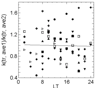
To consider the diurnal variations of k(t r, ave2) is a slightly more difficult task. We have seen above that for many stations not all local times were finally accepted for further averaging due to the three restrictions (criteria) super-imposed. For some stations there is some sort of k(t r, ave1) variation with LT, but no consistent picture is obtained for all stations. To illustrate this point we have drawn Fig. 5. For 8 high-latitude stations (the first 8 lines in Table 3) we have calculated for every LT moment (for which there was a k(tr, ave1) accepted) the ratio of this trend to the average value for this station k(t r, ave2) shown in Table 3. The ob-tained ratio is shown in Fig. 5. One can see from this figure that there is a scatter of the data but no systematic changes in the ratio (and this means of the k(tr, ave2)) with LT.
Thus, we may state that the trends obtained show no pro-nounced dependence on the geomagnetic latitude or local time. Both these dependencies are typical for the trends induced by the long-term changes in geomagnetic activity. Therefore, we may state that the trends derived in this paper are actually nongeomagnetic trends.
If we average the k(t r, ave2) values for 21 stations (ex-cluding Alma-Ata and Sodankyla) shown in Table 3, we
ob-Fig. 4. The nongeomagnetic trends k(tr, ave2) obtained for various
stations versus the modulus of the geographic latitude (points). The line represents the regression line through the data points. The bars correspond to the σ (2) values shown in Table 3.
Fig. 5. The ratio of the nongeomagnetic trend k(tr, ave1) de-rived for each LT moment to the daily mean value for this par-ticular station k(tr, ave2) versus local time. Stations used: Dik-son (dots), Loparskaya (diamonds), Lycksele (closed rectangles), Kiruna (closed triangles), Leningrad (open rectangles), Uppsala (crosses), Salekhard (inverted triangles), and Sodankyla (open tri-angles).
tain the value k(t r, ave3) = −0.0012 per year with the stan-dard deviation σ (3) = 0.0004. Thus, the k(t r, ave3) finally accepted is higher than 2σ . It shows that from 1958 to the middle of the 1990s the value of foF2 has been systemat-ically decreasing by 0.12% per year. If conventionally we
Table 4. Calculation of the trends for two periods for the Slough station
LT A B a1 C k(t r,ave1) σ(1) accepted comments
1958–1996 0 −0.54 −0.55 0.0034 0.010 −0.00146 0.00031 −0.00146 2 −0.67 −0.83 0.0044 −0.020 −0.00130 0.00022 −0.00130 4 −0.70 −0.87 0.0062 −0.007 −0.00110 0.00029 −0.00110 6 −0.70 −0.88 0.0062 0.021 −0.00110 0.00019 −0.00110 8 −0.71 −0.88 0.0064 0.004 −0.00083 0.00025 −0.00083 10 −0.59 −0.95 0.0031 −0.052 −0.00079 0.00008 −0.00079 12 −0.46 −0.75 0.0015 −0.035 −0.00068 0.00010 −0.00068 14 −0.30 −0.20 0.0009 0.018 −0.00066 0.00018 −0.00066 16 −0.25 −0.44 0.0013 0.033 −0.00104 0.00011 −0.00104 18 −0.27 −0.13 0.0012 0.046 −0.00156 0.00025 −0.00156 20 −0.35 −0.04 0.0015 0.007 −0.00163 0.00054 −0.00163 22 −0.49 −0.33 0.0028 −0.005 −0.00129 0.00042 −0.00129 R2= −0.93; R1= −0.75;
k(t r,ave2) = −0.000112 per year; σ (2) = 0.00034
1948–1985 0 −0.62 −0.90 0.0092 −0.008 −0.00041 0.00045 t r < σ 2 −0.71 −0.92 0.0120 −0.002 −0.00064 0.00042 −0.00064 4 −0.76 −0.94 0.0133 −0.004 −0.00062 0.00045 −0.00062 6 −0.74 −0.90 0.0095 0.007 −0.00022 0.00047 t r < σ 8 −0.75 −0.87 0.0078 −0.006 0.00015 0.00043 t r < σ 10 −0.60 −0.87 0.0054 −0.007 −0.00001 0.00033 t r < σ 12 −0.53 −0.84 0.0042 0.013 −0.00010 0.00022 t r < σ 14 −0.41 −0.67 0.0024 0.002 −0.00005 0.00026 t r < σ 16 −0.27 −0.69 0.0030 0.010 −0.00023 0.00025 t r < σ 18 −0.16 −0.67 0.0024 −0.011 −0.00060 0.00028 −0.00060 20 −0.47 −0.90 0.0073 0.001 −0.00076 0.00034 −0.00076 22 −0.59 −0.91 0.0082 0.007 −0.00057 0.00039 −0.00057 R2= −0.83; R1= −0.87; k(tr, ave2) = −0.00064; σ (2) = 0.00010;
A, B, and C denote the same as in Table 1
accept the average value of foF2 to be equal to 10 MHz, the above relative trend means an absolute decrease in the F2-layer critical frequency by 0.012 MHz per year.
The above value itself may seem small enough. But it means a decrease in foF2 from 1958 to the present day by about 0.5 MHz (if we compare identical conditions), which is not a very small value for the vertical sounding. However, as we have indicated in the Introduction, the main importance of detecting a nongeomagnetic trend is its very probable rela-tion to the problem of possible changes in the thermosphere due to an anthropogenic impact.
If the trends of foF2 detected are of an anthropogenic ori-gin, one can expect their change with the decades passing. For the analysis described above we have chosen the time interval after 1958 (see above Sect. 2: the method and data section). However, for some stations considered there are data for the earlier years, mainly from 1947. For these sta-tions we considered additionally the period 1948–1985 (for some stations the period began a year or two later, because the observations have started later) and compared the results with the trends shown in Table 3.
First of all, the difference was seen in the process of mak-ing the calculations. For many stations the picture for the 1948–1985 period is much less stable than for the 1958–1995 period. The trend k(t r) is less and the data scatter between various 30-year intervals is stronger, so for many LT mo-ments the k(t r, ave1) values are less than the standard devi-ation σ1. A comparison of the calculations for the Slough
station for the two periods is shown in Table 4. The dif-ference is visual: for the 1958–1996 period the trends for all 12:00 LT moments are higher than σ1, so all 12 values are
ac-cepted for the further averaging and they provided the value of k(t r, ave2) = −0.00112 per year with σ2 = 0.00034.
For the 1948–1985 period the trends for 00:04–16:00 LT are less than σ1, so only the k(t r, ave1) values for 18:00–
00:02 LT were acceptable for further averaging (except mid-night when the trend magnitude is only slightly less than σ ) which gave the value of k(t r, ave2) = −0.00064 per year with σ2=0.00010. Thus, for this particular station the trend
for the earlier time period (1948–1985) is found to be almost half that for the later period (1958–1996).
A. D. Danilov: Long-term trends of foF2 independent of geomagnetic activity 1175
Table 5. The trends derived for the earlier and later periods −k(t r,ave2) · 105 years of the station later earlier ratio earlier period Leningrad 125 81 1.54 1950-1985 Sverdlovsk 115 74 1.55 1948-1985 Tomsk 96 74 1.30 1948-1985 Moscow 96 61 1.57 1948-1985 Irkutsk 137 112 1.22 1949-1985 Slough 112 64 1.70 1948-1995 Canberra 163 76 2.14 1951-1985 Brisbne 65 1951-1985 average 121 75 1.57 σ(2) 24 17 0,30
the later and earlier periods (we have no data for the Brisbane station after 1985, so only the value for 1951–1985 is shown for this station). One can see that the difference in the trend values is systematic: for all stations considered the trends for the later years are higher than the trends for the earlier years. The ratio R varies between 1.30 and 2.14, with the average value of 1.56 and σ2=0.30. Thus, the
nongeomag-netic trends derived for the 1948–1985 period are by about a factor of 1.6 lower than the trends derived for the 1958–1995 period. We consider this fact as a very serious confirmation of the assumption that the nongeomagnetic trends have an anthropoginic origin.
We have already mentioned above that, as far as we had excluded the impact of two principal natural factors influ-encing foF2 long-term changes, we may believe that the non-geomagnetic trends obtained are of an anthropogenic origin. If this is true, one would expect an increase in these trends with time during the recent decades. This is exactly what we obtained by comparing the trends for 1948–1985 and for 1958–1995.
There is an obvious wish to simultaneously consider with the foF2 data the data on hmF2 as well. Unfortunately, the data on hmF2 are much more scarce. There is no data for the period before 1958, so the comparison of the later and earlier periods is impossible. However, the main problem is that the hmF2 data are much less reliable than the data on foF2. This fact is widely known and we are not going to go into details. We just mention that the consideration of the hmF2 relative trends (without excluding the geomagnetic activity effect) by Marin et al. (2001) shows that the picture with the
hmF2 trends is much less stable than with the foF2 trends.
Actually, the trends derived may depend even on the method used to recalculate the hmF2 values from the initial vertical sounding data.
All the above-said is aimed to explain why, in this paper, we deliberately avoided considering the hmF2 nongeomag-netic trends and prefered to limit ourselves only by the foF2 trends. The hmF2 trends need special consideration.
5 Conclusions
The method proposed by the author earlier (Danilov, 2002b) was applied to the foF2 observations in the period between 1958 and the mid-nineties at 23 ionospheric stations located at middle and high latitudes of the eastern hemisphere, to derive the long-term trends independent of geomagnetic ac-tivity. The results obtained are quite consistent: for all 23 stations the trend is negative. If we withdraw the results for two stations (Alma-Ata and Sodankyla, providing a strong deviation of the k(t r, ave2) from the value for other stations, the k(t r, ave2) for the rest of 21 stations lies within the inter-val from −0.00062 to −0.00196 per year.
No variations of the nongeomagnetic trend derived are found with geomagnetic and geographic latitude, or local time. This makes it possible to average the k(t r, ave2) val-ues for all 21 stations, to derive the mean trend k(t r, ave3) = −0.0012 per year with the standard deviation σ (3) = 0.0004. The analysis of the data since 1948, available for a few stations, shows that the trends for the period 1948–1985 are less (on the average, by a factor of 1.6) than for the period between 1958 and the mid-nineties. This fact is a strong ar-gument in favor of the assumption that the nongeomagnetic trends derived are of an anthropogenic origin and manifest long-term changes in thermospheric parameters due to the upper atmosphere contamination.
A detailed discussion of the problem of the long-term changes in the upper atmosphere is out of the scope of this paper. We refer the readers to the Proceedings of the Second Workshop on the Trends in the Atmosphere (Prague, July 2001) in a special issue of the Journal of Physics and Chem-istry of the Earth (2002). Here we mention two pertinent points.
First, there is little doubt now that there are long-term changes in the upper mesosphere (including a temperature trend). These changes should be inevitably manifested in long-term trends of thermospheric parameters. Some authors even claim a “subsidence” of the entire upper atmosphere.
There is a paper by Keating et al. (2000) in which some confirmation of the assumption of long-term changes in the thermosphere is obtained on the basis of the many-year satel-lite observations. If there is a depletion of the density at the 350 km height derived by Keating et al. (2000), one should expect changes in other thermospheric parameters at the F2-layer height which may lead to changes in foF2 and hmF2. The results obtained in this paper may be one of the manifes-tations of these changes.
Acknowledgements. The author thanks Prof. A. V. Mikhailov for
developing the computer program used in the calculations described in this paper and for his help in collecting the foF2 data.
Topical Editor M. Lester thanks M. Jarvis and another referee for their help in evaluating this paper.
References
Bencze, P., Sole, G., Alberca, L. F., and Poor, A.: Long-term changes of hmF2 possible latitudinal and regional variations, Proc. of the 2nd COST 251 Workshop “Algorithms and Models for COST 251 Final Product”, 30–31 March 1998, Side Turkey, Rutherford Appleton Lab.,UK, 107–113, 1998.
Bremer, J.: Some additional results of long-term trends in vertical-incidence ionosonde data, Paper presented at the COST 251 Meeting, Prague, September 1996.
Bremer, J.: Trends in the ionospheric E- and F-regions over Europe, Ann. Geophysicae, 16, 986–996, 1998.
Bremer, J.: Trends in the thermosphere derived from global ionosonde observations, Adv. Space Res., 28 (7), 997–1006, 2001.
Danilov, A. D.: F-region response to geomagnetic storms, J. Atmos. Sol-Terr. Phys., 63, 441–449, 2001.
Danilov, A. D.: Overview of the trends in the ionospheric E- and F2-regions, Phys. Chem. Earth (C)., 579–588, 2002a.
Danilov, A. D.: The method of determination of the long-term trends in the F2-region independent of geomagneic activity, Ann. Geophysicae, 20, 1–11, 2002b.
Danilov, A. D. and Mikhailov, A. V.: Long-term trends of the F2-layer critical frequencies: a new approach, Proc. of the 2nd COST 251 Workshop “Algorithms and Models for COST 251 Fi-nal Product”, 30–31 March, 1998, Side Turkey, Rutherford Ap-pleton Lab., UK, 114–121, 1998.
Danilov, A. D. and Mikhailov, A. V.: Spatial and seasonal variations of the foF2 long-term trends, Ann. Geophysicae, 17, 1239–1243, 1999.
Danilov, A. D. and Mikhailov, A. V.: Analysis of the Argentine Is-lands and Port Stanley vertical sounding data, Ann. Geophysicae, 19, 1–9, 2001.
Givishvili, G. V. and Leshchenko, L. N.: Long-term trends of the properties of the midlatitude ionosphere and thermosphere, Dokl. RAN (in Russian), 333 (1), 86–89, 1993.
Givishvili, G. V. and Leshchenko, L. N.: Possible proof of the
presence of technogenic impact on the midlatitude ionosphere, Dokl. RAN (in Russian), 334 (2), 213–214, 1994.
Jarvis, M. J., Jenkins, B., and Rogers, G. A.: Southern hemisphere observations of a long-term decrease in F-region altitude and thermospheric wind providing possible evidence for global ther-mospheric cooling, J. Geophys. Res., 103 (20), 744–787, 1998. Keating, G. M., Tolson, R., and Bradford, M. S.: Evidence on
long-term global decline in the Earth’s atmosphere densities appar-ently related to anthropogenic effects, Geophys. Res. Lett., 27 (10), 1523–1526, 2000.
Marin, D., Mikhailov, A. V., de la Morena, B. A., and Herraiz, M.: Long-term hmF2 trends in the Eurasian longitudinal sector on the ground-based ionosonde observations, Ann. Gophysicae, 19, 761–772, 2001.
Mikhailov, A. V. and Marin, D.: Geomagnetic control of the foF2 trends, Ann. Geophysicae, 18, 653–665, 2000.
Mikhailov, A. V. and Marin, D.: An interpretation of the foF2 and
hmF2 long-term trends in the framework of the geomagnetic
con-trol concept, Ann. Geophysicae, 19, 743–748, 2001.
Proells, G.: Ionospheric F-region storms, in: Handbook of Atmo-spheric Eletrodynamics, Vol. 2, (Ed) Volland, H., CRC Press, Boka Raton, pp. 195–248, 1995.
Tobiska, W. K., Woods, T. N., Eparvier, F. G., and Bouwer, S. D.: Validation of the 10.7 proxy produced by SOLAR2000, Pa-per presented at the 33th COSPAR Scientific Assembly, Warsaw, Abstracts, p. 89, 2000.
Ulich, T. and Turunen, E.: Evidence for long-term cooling of the upper atmosphere in ionospheric data, Geophys. Res. Lett., 24, 1103–1106, 1997.
Ulich, T., Karinen, A., and Turunen, E.: Effects of solar variability seen in long-term EISCAT radar observations of the lower iono-sphere, Paper presented at the Second IAGA/CMA Workshop on Solar Activity Forcing of the Middle Atmosphere, Prague, Au-gust 1997.
Upadhyay, H. M. and Mahajan, K. K.: Atmospheric greenhouse effect and ionospheric trends, Geophys. Res. Lett., 25, 3375– 3378, 1988.