HAL Id: hal-01162688
https://hal.inria.fr/hal-01162688
Submitted on 11 Jun 2015
HAL is a multi-disciplinary open access
archive for the deposit and dissemination of
sci-entific research documents, whether they are
pub-lished or not. The documents may come from
teaching and research institutions in France or
abroad, or from public or private research centers.
L’archive ouverte pluridisciplinaire HAL, est
destinée au dépôt et à la diffusion de documents
scientifiques de niveau recherche, publiés ou non,
émanant des établissements d’enseignement et de
recherche français ou étrangers, des laboratoires
publics ou privés.
Velocity estimation of valve movement in oysters for
water quality surveillance
Hafiz Ahmed, Rosane Ushirobira, Denis Efimov, Damien Tran, Jean-Charles
Massabuau
To cite this version:
Hafiz Ahmed, Rosane Ushirobira, Denis Efimov, Damien Tran, Jean-Charles Massabuau. Velocity
estimation of valve movement in oysters for water quality surveillance. IFAC MICNON 2015, Jun
2015, Saint-Petersburg, Russia. �hal-01162688�
Velocity estimation of valve movement in
oysters for water quality surveillance
Hafiz Ahmed∗ Rosane Ushirobira∗ Denis Efimov∗,∗∗,∗∗∗ Damien Tran∗∗∗∗ Jean-Charles Massabuau∗∗∗∗
∗Non-A team at Inria, Parc Scientifique de la Haute Borne, 40 avenue Halley, 59650 Villeneuve d’Ascq, France (e-mail: hafiz.ahmed,
rosane.ushirobira, denis.efimov@inria.fr)
∗∗CNRS UMR 9189 CRIStAL, Ecole Centrale de Lille, Avenue Paul Langevin, 59651 Villeneuve d’Ascq, France
∗∗∗Department of Control Systems and Informatics, Saint Petersburg State University of Information Technologies Mechanics and Optics
(ITMO), 49 av. Kronverkskiy, 197101 Saint Petersburg, Russia ∗∗∗∗EA team at CNRS UMR 5805 EPOC, Universit Bordeaux 1,
OASU, Bordeaux, France (e-mail: d.tran, jc.massabuau@epoc.u-bordeaux1.fr)
Abstract: The measurements of valve opening activity in a population of oysters under natural environmental conditions are used to estimate the velocity of their valve movement activity. Three different differentiation schemes were used to estimate the velocity, namely an algebraic-based differentiator method, a non-homogeneous higher order sliding mode differentiator and a homogeneous finite-time differentiator. The estimated velocities were then used to compare the performances of these three different differentiators. We demonstrate that this estimated velocity can be used for water quality monitoring as the differentiators can detect very rapid change in valve movements of the oyster population resulting from some external stimulus or common input.
Keywords: Velocity estimation, water quality monitoring, Oyster population.
1. INTRODUCTION
Since the last century, the environmental quality of our world is changing rapidly causing significant changes in the water quality. For this reason, nowadays, national and international legislation has strict recommendations on the protection of aquatic environment against the re-lease of dangerous substances. In order to abide by these recommendations for the protection of aquatic environ-ments, the large scale monitoring of water quality is es-sential. However, to implement such an extensive network of monitoring is very costly. Researchers are then work-ing on an indirect ecological monitorwork-ing from behavioral and physiological responses of representatives of the ma-rine fauna. Hence, bio-indicators are increasingly being used and showed high efficiency, for instance through bio-accumulation of contaminants in their tissues. Neverthe-less, until now, large scale monitoring with bio-indicators do not seem feasible and realistic as it involves inten-sive exploitation of human resources for the collection of samples, complex chemical analysis and so on [Telfer et al. (2009)]. A solution is to develop unmanned systems using bio-sensors, able to work 24/7, at high frequency
1 Hafiz Ahmed is partially supported by the regional council of
Nord-Pas de Calais, France. This work was supported in part by the Government of Russian Federation (Grant 074-U01) and the Ministry of Education and Science of Russian Federation (Project 14.Z50.31.0031)
by remote control. As of today, networks of such online sensors, operating at large scale do not exist and are still a matter of research.
To fulfill that objective, an installation of numerous online remote sensors is required, working at high frequency for instant collection of information on a daily basis in marine environment [Krger and Law (2005)]. Behavioral and phys-iological responses of wildlife to pollution are very sensitive and can be estimated for an indirect ecological monitoring. However, a limiting factor today is the analysis of data that needs sufficiently accurate models of animal behavior in natural conditions. Other difficulties lie in the fact that animals may be heavily influenced by environment, group interactions and internal rhythms (e.g. feeding, breathing, spawning).
Observation of the opening and closing activities of bi-valves is a possible way to evaluate their physiological behavior in reaction to environment. The deviations from a normal behavior can be used for detection of a con-taminant in surrounding water. The pioneer work that analyzes bivalve’s activities through the record of their valve movements (e.g. valvometry) was realized by F. Marceau [Marceau (1909)] with smoked glazed paper. Today, valvometers are commercially available and are mainly based on the principle of electromagnetic induc-tion, like the Mossel Monitor [Kramer et al. (1989)] or the Dreissena Monitor [Borcherding (1992)]. In recent years,
the interest for modeling and estimation of behavior of marine animals directly in real marine conditions has in-tensively increased [Riisgard et al. (2006); Robson et al. (2007); Garcia-March et al. (2008); Galang et al. (2012)]. A remarkable monitoring solution has been realized in the UMR CNRS 5805 EPOC Laboratory in Arcachon, France [Sow et al. (2011); Tran et al. (2003); Schmitt et al. (2011)], where a new framework for noninvasive valvometry has been developed and implemented since 2006. The designed method is strongly based on bivalve’s respiratory physiology and ethology. The developed plat-form for valvometry was built using lightweight electrodes (approximately 100 mg each) linked by thin flexible wires to high-performance electronic units. These electrodes are capable to measure the position of the opening of a mollusk shell with an accuracy of a few µm. This system allows the bivalves to be studied in their natural environment with minimal experimental constraints. Statistical approaches have already been used for the analysis of this data [Sow et al. (2011); Tran et al. (2003); Schmitt et al. (2011)]. The goal of the present work is to estimate the velocity of the valve opening/closing activities of the bivalve (i.e. an oyster in our case) from the measured position of shell. We have used the experimental data obtained from a population of 16 oysters living in the bay of Arcachon (France). We have tried to examine whether there exist any relationship between the velocity and the contamination of water as the quality of the water influence the behavior of the oyster population. Three different methods of differ-entiation were used for estimating the velocity, namely: an algebraic differentiator [Mboup et al. (2009)], a higher order sliding mode (HOSM) based differentiator [Efimov and Fridman (2011)] and a homogeneous finite-time dif-ferentiator [Perruquetti et al. (2008)]. Their performances were then compared. The methods were chosen because of their individual merits. For example, HOSM differentiator has the global differentiation ability independently on the amplitude of the differentiated signal and measurement noise, but it has some chattering in the response, while the homogeneous finite-time differentiator has no chat-tering, but it is more sensitive to the amplitudes of the signals to be differentiated. The differentiator based on the aforementioned algebraic method is very useful in noisy settings, but it presents some delay in online applications. The organization of the paper is as follows: a brief de-scription on the measurement and data collection activity is given in section II. Section III presents a summarized version of the three differentiation schemes, while section IV describes the result, i.e velocity estimation from the experimental data, and discusses the relation of velocity estimation with contamination level in water. Finally, sec-tion V concludes the present work.
2. MEASUREMENT SYSTEM DESCRIPTION The monitoring site was located in the bay of Arcachon, France, at the Eyrac pier (Latitude: 44◦40 N, Longitude: 1◦10 W). Sixteen Pacific oysters, Crassostrea gigas, mea-suring from 8 cm to 10 cm in length were permanently installed on this site. These oysters were all from the same age group (1.5 years old) and came from the same local supplier. They also all grew in the bay of Arcachon. They
were immersed on the sea bottom (at 3 m to 7 m deep in the water, depending on the tide activity). We analyzed the data for the year 2007.
The electronic equipment has been first described in [Tran et al. (2003)] and slightly modified (adapted to severe open ocean conditions) in [Chambon et al. (2007)]. A considerable advantage of this monitoring system is that it is completely autonomous and made to work without in
situ human intervention for one full year. Each animal is
equipped with two light coils (sensors) of approximately 100 mg each, fixed on the edge of each valve. One of the coils emits a high-frequency sinusoidal signal, that is received by the other coil. One measurement is performed every 0.1 sec (i.e. at 10 Hz) for one among the sixteen animals. So the behavior of a particular oyster is measured every 1.6 sec. EPOC’s website MolluScan-Eye2 can be consulted to see the recorded data sets of information. So, every day, 54000 triplets (1 distance, 1 stamped time value, 1 animal number) are collected for each oyster. The strength of the electric field produced between the two coils is proportional to the inverse of distance between the point of measurement and the center of the transmitting coil leading to the measurement of the distance between coils. A schematic description of the monitoring system can be found in [Ahmed et al. (2014, 2015)].
3. DIFFERENTIATION METHODS
For our problem of velocity estimation of the valve activity in oysters, we have considered three different methods of derivative estimation that are summarized below.
3.1 Algebraic differentiator
The algebraic time derivative estimation presented here is based on concepts of differential algebra and operational calculus. A more detailed description of the approach can be found in [Mboup et al. (2009); Ushirobira et al. (2013)]. A moving horizon version of this technique is summarized below adapted from the references mentioned just before. For a real-valued signal y(t), analytic on some real interval, consider its approximating N th degree polynomial func-tion, originated from its truncated Taylor expansion:
y(t) = N ∑ i=0 ai i!t i, (1)
where the terms ai’s are the unknown constant coefficients
representing the derivatives of the signal. The aim is to estimate these time derivatives of y(t), up to order N . This estimation can be done by restarting the algebraic combinations on moving time horizon of integrals of y(t). The summarized result of this method is given below taken from [Mboup et al. (2009)]:.
For any T > 0, the j-th order time derivative estimate by(j)(t), j = 0, 1, 2,· · · , N, of the signal y(t) defined in (1)
satisfies the following convolution by(j)(t) = ∫ T 0 Hj(T, τ )y(t− τ)dτ, j = 0, 1, · · · , N, 2 http://molluscan-eye.epoc.u-bordeaux1.fr/
for all t≥ T , where the convolution kernel, Hj(T, τ ) = (N + j + 1)!(N + 1)! TN +j+1 × N∑−j κ1=0 j ∑ κ2=0 (T− τ)κ1+κ2(−τ)N−κ1−κ2 κ1!κ2!(N− κ1− κ2)!(κ1+ κ2)!(N− κ1+ 1) .
As we can conclude, the kernel Hj(T, τ ) depends on the
order j of the time derivative to be estimated and on an arbitrary constant length of time window, T > 0. Since we are interested in calculating the first-order time derivative, let us consider a degree-one polynomial y(t) = a0+ a1t.
By applying the above result to this signal, we obtain the following first-order time derivative estimate
b˙y(t) =∫ T
0
6
T3(T− 2τ)y(t − τ)dτ. (2)
3.2 A non-homogeneous HOSM differentiator
The differentiation problem in this case has the following setup: let us consider an unknown signal y(t). To calculate the derivative of this signal, consider an auxiliary equation
˙
x = u where x(t) denotes the estimate of the original
signal y(t). The control law u is designed to drive the estimation error, i.e. e(t) = x(t)− y(t), to zero. The work [Efimov and Fridman (2011)] proposes a variant of a super-twisting finite-time control u that ensures vanishing the error e(t) and its derivative ˙e(t). Thus it can be used to provide a derivative estimate. It has also been shown that the obtained estimate is robust against a non-differentiable noise of any amplitude. Now if we consider a noisy version of the original signal i.e. ˜y(t) = y(t) + ν(t), where ν(t) is
a bounded measurement noise, then the differentiator is given by [Efimov and Fridman (2011)]:
˙ x1=−α √ |x1− ˜y(t)| sgn (x1− ˜y(t)) + x2, (3) ˙ x2=−β sgn (x1− ˜y(t)) − χ sgn (x2)− x2,
where x1, x2∈ R are the state variables of the system (3),
α, β and χ are the tuning parameters with α > 0 and β > χ≥ 0. The variable x1(t) serves as an estimate of the
function y(t) and x2(t) converges to ˙y(t), i.e. it provides
the derivative estimate. Therefore the system (3) has ˜y(t)
as the input and x2(t) as the output.
Moreover, the system (3) is discontinuous and affected by the disturbance ν. So, the first thing to prove is that the system has bounded trajectories. The second important point is to check the quality of the derivative estimation with respect to noise amplitude. To proceed, introduce new variables e1 = x1(t)− y(t) and e2 = x2(t)− ˙y(t). The
system (3) can now be written with respect to the new variables as: ˙ e1=−α √ |e1| sgn (e1) + δ1(t), ˙ e2=−γ(t) sgn (e1)− χ sgn (e2)− e1+ δ2(t), (4) δ1(t) = α √ |e1| sgn (e1)− (√ |e1− ν(t)| sgn (e1− ν(t)) ) , δ2(t) = β (sgn (e1)− sgn (e1− ν(t))) ,
where the disturbances originated from the noise ν are
δ1 and δ2 and the function γ(t) = β + ( ˙y(t) + ¨y(t))−
χ (sgn (e2(t))− sgn (e2(t) + ˙y(t))) sgn (e2(t)) is piecewise
continuous. If| ˙y(t)| ≤ ℓ1,|¨y(t)| ≤ ℓ2, for example, then for
β > ℓ1+ℓ2+2χ, it is strictly positive and 0 < δ≤ γ(t) ≤ κ
for δ = β−ℓ1−ℓ2−2χ and κ = β+ℓ1+ℓ2+2χ. Assume that
|ν(t)| ≤ λ0 for all t∈ R+. By definition,|δ1(t)| ≤ α
√
2λ0,
δ2(t) = 0 for|e1(t)| ≥ λ0, |δ2(t)| ≤ 2β and δ2(t)e1(t)≥ 0
for all t∈ R+. Then the global boundedness of the
solu-tions of the differentiator (4) is given by the next Lemma.
Lemma 1. (Efimov and Fridman (2011)). Let the signal ν : R → R be Lebesgue measurable and | ˙y(t)| ≤ ℓ1,
|¨y(t)| ≤ ℓ2, |ν(t)| ≤ λ0 for all t∈ R+; α > 0, β > 0 and
0 < χ < β. Then in (4) for all t0∈ R+and initial conditions
x1(t0)∈ R, x2(t0)∈ R the solutions are bounded:
|x1(t)− y(t)| < max { |x1(t0)− y(t0)|, 4α−2(|x2(t0)− ˙y(t0)| +3β + ℓ1+ ℓ2+ χ + α √ 2λ0)2 } , |x2(t)− ˙y(t)| ≤ |x2(t0)− ˙y(t0)|e−0.5t+|3β + ℓ1+ ℓ2+ χ|,
This Lemma states that the proposed differentiator has bounded solution for any positive values of the tuning parameters α, β and χ and all initial conditions. The accuracy of the derivative estimation in the case of non-differentiable noise is analyzed in the following. The prop-erties of the signal ν(t) are the same as in Lemma 1.
Lemma 2. (Efimov and Fridman (2011)). Let β > ℓ1 +
ℓ2+2χ, χ > 0 and α≥ 2
(√
8κχ +√χ + κ(κ− δ))/(1.5δ+
0.5κ). Then for any initial conditions e(0) ∈ Ω0 =
{ e∈ R2: κ|e 1(0)| + 0.5e22(0)≤ 2 √ 2κ(χ + κ)χδ(κ− δ)−1 } , the trajectories of the system (4) satisfy the estimate for all
t≥ T |e1(t)| ≤ δ−1 ( c1λ0+ c2 √ λ0 ) , |e2(t)| ≤ √ 2 ( c1λ0+ c2 √ λ0 ) , c1= max { 8 µ2 ( (0.025δ + κ)α + max{√2(χ + κ), 6 } β )2 , κ } , c2= β2/(α √ 2), µ = min{αδ/√κ,√2χ}
where the finite time T of convergence possesses the estimate T ≤ 4µ−1√κ|e1(0)| + 0.5e22(0), provided that
c1λ0+ c2
√ λ0≤ 2
√
2κ(χ + κ)χδ(κ− δ)−1.
The result of Lemma 2 says that if the noise amplitude λ0
is comparable with the chosen α, β and γ (the constraint
c1λ0+ c2
√ λ0≤ 2
√
2κ(χ + κ)χδ(κ− δ)−1holds), then the resulted estimate x2on the derivative ˙y has the error
pro-portional to λ0.50 and λ0.250 . If the noise amplitude is very
high, then the result of Lemma 1 satisfies guaranteeing the boundedness of the trajectory.
3.3 Homogeneous finite-time differentiator
Consider a nonlinear system of the following form: ˙
x = η(x, u), (5)
y = h(x), (6)
where x ∈ Rd is the state, u ∈ Rn is a known and
sufficiently smooth control input and y(t) ∈ R is the output. The function η : Rd × Rm → Rd is a known continuous vector field. It is assumed that the system
described by (5)–(6) is locally observable and there exists a local coordinate transformation that transforms the system (5)–(6) into the observable canonical form
˙
z = Az + f (y, u, ˙u, . . . , u(r)), (7)
y = Cz,
where z∈ Rnis the state, r > 0 and
A = a1 1 0 0 0 a2 0 1 0 0 . . . . . . . . . . .. ... an−1 0 0 0 1 an 0 0 0 0 , C = ( 1 0 · · · 0). (8)
The observer design for the transformed system then becomes simple as all the nonlinearities are now functions of output and known input.
The notions of finite time stability and homogeneity used here are omitted due to space limitation and can be consulted from [Perruquetti et al. (2008)]. An observer can be designed as follows dˆz1 dt dˆz2 dt . . . dˆzn dt = A z1 ˆ z2 . . . ˆ zn + f (y, u, ˙u,· · · , u(r))− χ1(z1− ˆz1) χ2(z1− ˆz1) . . . χn(z1− ˆz1) ,
where the functions χi’s are defined in a way that
the observation error e = z − ˆz tends to zero in a finite time (an example is given below). According to [Perruquetti et al. (2008)], an approach to ensure FTS is based on homogeneity. The observation error dynamics can be written as ˙ e1 = e2+ χ1(e1), ˙ e2 = e3+ χ2(e1), .. . ˙en−1, en+ χn−1(e1), ˙ en = χn(e1). (9)
Denote ⌈x⌋ = |x|αsgn(x) for all x ∈ R and some α >
0, then select χi(e1) = −ki⌈e1⌋αi,1 ≤ i ≤ n − 1 for
coefficients k1, ..., kn forming a Hurwitz polynomial and
the powers (α1, ..., αn)∈ Rn>0have to be selected to ensure
that the system (9) is homogeneous with respect to some (r1, ..., rn) ∈ Rn>0. For a given d ∈ R, the sequences
(r1, ..., rn) and (α1, ..., αn) can be chosen via the following
recurrent formulas: ri+1= ri+ d, 1≤ i ≤ n − 1, αi= ri+ 1 r1 , 1≤ i ≤ n − 1, αn= rn+ d r1 ,
then the system (9) is homogeneous of degree d w.r.t. the weights (r1, ..., rn) ∈ Rn>0 [Perruquetti et al. (2008)]. A
particular choice is ri={(i − 1)α − (i − 2)} and αi= iα−
(i−1) for all 1 ≤ i ≤ n for some α ∈ [
1−n−11 , 1
]
, then (9) is homogeneous of degree α− 1 [Perruquetti et al. (2008)]. Therefore, the system (9) can be then written as follows
˙ e1 = e2− k1⌈e1⌋α, ˙ e2 = e3− k2⌈e1⌋2α−1, . . . ˙ en−1 = en− kn⌈e1⌋(n−1)α−(n−2), ˙ en = kn⌈e1⌋nα−(n−1).
Theorem 3. (Perruquetti et al. (2008)). For any coefficients k1, . . . , kn forming a Hurwitz polynomial, there exists
α∈
[
1−n−11 , 1
]
(sufficiently close to 1) such that (9) is globally FTS.
The advantages of homogeneous finite-time stable systems include the rate of convergence and their robustness with respect to different disturbances.
Using the designed observer, a differentiator can be de-rived. For this purpose consider a smooth signal y(t). The aim of the differentiator is to estimate the successive time derivatives of y(t) up to the order n− 1, i.e. ˙y(t), . . . ,
y(n−1)(t). Assume that y(n)(t) = θ(y(t), . . . , y˙ (n−1)(t)).
Set Y =[y y˙ · · · y(n−1)]T. Then,
˙
Y = AY + Θ(Y ), y = CY,
where A and C can be found in (8) and
Θ(Y ) = 0 . . . 0 θ(y(t), ..., y˙ (n−1)(t)) ∈ Rn.
So, the following homogeneous finite-time observer (which is a differentiator in this case) can be proposed:
˙
z1= z2− k1⌊z1− y⌉α,
˙
zi= zi+1− k⌊z1− y⌉iα−(i−1), i = 2, . . . , n− 1,
˙
zn=−kn⌊z1− y⌉nα−(n−1).
4. RESULT AND DISCUSSIONS
As mentioned in the Introduction, the goal of this paper is to estimate the velocities of the valve opening/closing activities of an oyster population for ecological monitor-ing. The activity of an oyster population was observed in the bay of Arcachon, France. The water quality of our experimental site was fairly the same throughout the year. Therefore, the behavior of the population was about the same as their natural behavior. However, during the Win-ter, excessive rainfall was observed from mid-November to mid-December in the bay of Arcachon in 2007. This can be seen as a perturbation for the oysters. As a consequence, we may expect that this perturbation would change the behavior of the oyster population resulting in a rapid open-ing/closing of the valves. This would imply an increase of the velocity, as velocity is nothing but the time derivative of the distance of the valve opening/closing.
The valve opening/closing activity of the oyster population can be seen in Fig. 1. Once we have the data of the distance of the valve opening/closing, we can estimate the velocity
0 10th December 20th December 30th December 0 0.1 0.2 0.3 0.4 0.5 0.6 0.7 0.8
Days of the Month of December
normalized valve distance
Fig. 1.Valve opening/closing activity of the oyster population for the month of December in the bay of Arcachon, France
0 5 10 15 20 25 30 −1.2 −1 −0.8 −0.6 −0.4 −0.2 0 0.2 0.4 0.6 0.8
Days of the month of December
Normalized valve distance and speed
Signal Speed−HOSM Speed−HOMD Speed−ALM
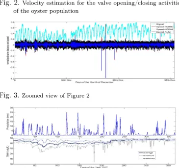
Fig. 2.Velocity estimation for the valve opening/closing activities of the oyster population
Fig. 3.Zoomed view of Figure 2
Fig. 4.Precipitation and water salinity level in the bay of Arcachon in 2007
of this activity using the methods described in Section 3. The estimated valve velocity of the oyster population (a mean value for all oysters) is given in Fig. 2, while the data regarding the precipitation and water salinity level in the bay of Arcachon during 2007 can be seen in Fig. 4. Fig. 2 contains 1.5425 million data points. Now, if we take a closer look at the figure by zooming it, the velocity estimation performance of the different differentiators can be observed more precisely. A close-look of Fig. 2 can be seen in Fig. 3. From this last figure, it can be con-cluded that the three differentiators are producing roughly the same result. HOSM differentiator is affected by the chattering effect, but in spite of this fact, the output of HOSM differentiator is very much similar to the output of Homogeneity based differentiator. The output of algebraic method based differentiator is a little delayed, but it is smoother than the others. From the output of the three
0 11h 13m 11h 27m 11h 40m 11h 53m 0.2 0.3 0.4 0.5 0.6 0.7 0.8 0.9 Time in minutes
normalized valve distance
Fig. 5.Valve opening/closing activity of the population on Decem-ber 17 between 11.00 hour and 12.00 hour
differentiators, no definitive conclusion can be drawn by saying that a certain differentiator is the best in our case as no reference is achievable (no quantitative evaluation). However, a qualitative assessment can be performed: since HOSM and homogeneity based differentiator both recon-struct/estimate the original signal to calculate its time derivative, a qualitative comparison is possible between them by looking at the original signal estimation error. This approach is not applicable for the algebraic differen-tiator. For HOSM, the estimation error was 0.22% while for Homogeneity based differentiator it was 0.35%. As mentioned before, some heavy rainfall was observed at the beginning of December and it could be considered as a potential perturbation for the oysters. From the figures, we can see that no abnormal/sudden rapid change in velocity can be observed within these days. The velocity pattern starting from the beginning of December and onward seems quite normal. So, no direct relationship between the valve opening/closing activity and the perturbation (i.e. heavy rainfall) was established here. One reason for this is maybe the data itself, for example, if some dynamics is missing. Our data acquisition system spends 0.1 sec for each oyster and continues this for the rest of the population. So, the next time it returns to the same oyster when 1.6 sec is already past and we do not have any information within this period. It has been observed in the laboratory environment that oysters can respond more rapidly to a perturbation in the water quality. Amplitude/level of perturbation along with other environmental factors like, tide, sun, cloudiness, etc., play a role in their response to perturbations as well. All these possibilities plus an improved data acquisition system should be considered for a future study.
A final remark is that an abnormal increase in the pop-ulation velocity of valve activity has been detected by the system later on between December 17 & 18. Most individuals in the population closed their valve rapidly in unison as it can be better observed by the zoom of the population activity in Fig. 5. From this figure, we can tell that the members of the population suddenly closed their valve around 11 hour 26 minutes. Before, we didn’t observe any such rapid valve movement in unison. That is why it can’t be said that this behavior is due to some internal dynamics of the individual oysters. We can conclude that they all shared/influenced by some common input/external stimulus. However, the origin of this com-mon input/external stimulus is still not known to us. In terms of the effectiveness of our differentiators, it can be said from Fig. 2 that they are quite capable of detecting this sudden rapid closing of the valve of the population which happened in just few seconds. This was the aim of our work i.e. to detect the rapid movement of the valve
activity by which we can monitor the water quality. In that sense, we can tell that our work is quite successful in case of the detection of the rapid change in valve activity which can be a way to monitor the water quality.
5. CONCLUSION
This paper presents the application of three different veloc-ity estimators to estimate the valve movement activveloc-ity of an Oyster population for ecological monitoring, i.e. water quality surveillance. The behavior of the population of 16 oysters was normalized and averaged to generate the behavior of the population. This data was then used to estimate the velocities. The three different velocity esti-mators were: algebraic-based method differentiator, non-homogeneous higher order sliding mode differentiator and homogeneous finite-time differentiator. Their performance was satisfactory in estimating the velocity of the oyster population. Their output was more or less almost the same. This estimated velocity was then used to monitor the water quality as the valve movement activity depends on this. It was shown that the velocity estimators were capable of detecting the rapid change in valve movement due to the synchronous behavior of oyster population to some common input/external stimulus. This capability of detecting the rapid change can be used for monitoring the water quality by using the oysters as biosensors.
This work has some limitation because of the data being used as it was discussed in the previous Section. In future works, the estimators have to be tested using the data providing more information than the current one so that every possible dynamics of the oyster population is preserved in the data set. Moreover, the same approach,
i.e. velocity estimation, can be considered for detecting
other phenomenon like spawning in a future work.
Acknowledgment The authors thank Ifremer Arcachon and Isabelle Auby for kindly providing precipitation and salinity data for the Eyrac pier, Bay of Arcachon, 2007.
REFERENCES
Ahmed, H., Ushirobira, R., Efimov, D., Tran, D., and Massabuau, J.C. (2014). Dynamical model identification of population of oysters for water quality monitoring. In Control Conference (ECC), 2014 European, 152–157. doi:10.1109/ECC.2014.6862479.
Ahmed, H., Ushirobira, R., Efimov, D., Tran, D., Sow, M., and Massabuau, J.C. (2015). Automatic spawning detection in oysters: a fault detection approach. In Proc.
European Control Conference (ECC) 2015.
Borcherding, J. (1992). The Zebra Mussel Dreissena Polymorpha: Ecology, Biological Monitoring and First Applications in the Water Quality Management, chapter
Another early warning system for the detection of toxic discharges in the aquatic environment based on valve movements of the freshwater mussel Dreissena polymor-pha, 127–146. Gustav Fischer Verlag, NY.
Chambon, C., Legeay, A., Durrieu, G., Gonzalez, P., Ciret, P., and Massabuau, J.C. (2007). Influence of the parasite worm polydora sp. on the behaviour of the oyster crassostrea gigas: a study of the respiratory impact and associated oxidative stress. Marine Biology, 152(2), 329– 338.
Efimov, D. and Fridman, L. (2011). A hybrid robust non-homogeneous finite-time differentiator. Automatic
Control, IEEE Transactions on, 56(5), 1213–1219. doi:
10.1109/TAC.2011.2108590.
Galang, G., Bayliss, C., Marshall, S., and Sinnott, R.O. (2012). Real-time detection of water pollution using biosensors and live animal behaviour models. In
eRe-search Australasia: emPower eReeRe-search. Sydney,
Aus-tralia.
Garcia-March, J., Sanchis Solsona, M., and GarciaCarras-cosa, A. (2008). Shell gaping behavior of pinna nobilis l., 1758: Circadian and circalunar rhythms revealed by in situ monitoring. Marine Biology, 153, 689–698. Kramer, K.J.M., Jenner, H.A., and De Zwart, D. (1989).
The valve movement response of mussels: A tool in biological monitoring. Hydrobiologia, 188/189, 433–443. Krger, S. and Law, R. (2005). Sensing the sea. Trends in
Biotechnology, 23, 250–256.
Marceau, F. (1909). Contraction of molluscan muscle.
Arch. Zool. Exp. Gen., 2, 295–469.
Mboup, M., Join, C., and Fliess, M. (2009). Numerical differentiation with annihilators in noisy environment.
Numerical Algorithms, 50(4), 439–467.
Perruquetti, W., Floquet, T., and Moulay, E. (2008). Finite-time observers: Application to secure communica-tion. Automatic Control, IEEE Transactions on, 53(1), 356–360.
Riisgard, H., Lassen, J., and Kittner, C. (2006). Valvegape response times in mussels (mytilus edulis): Effects of laboratory preceding feeding conditions and in situ tidally induced variation in phytoplankton biomass. The
Journal of Shellf ish Research, 25, 901–911.
Robson, A., Wilson, R., and Garcia de Leaniz, C. (2007). Mussels flexing their muscles: A new method for quanti-fying bivalve behavior. Marine Biology, 151, 1195–1204. Schmitt, F.G., De Rosa, M., Durrieu, G., Sow, M., Ciret, P., Tran, D., and Massabuau, J.C. (2011). Statistical study of bivalve high frequency microclosing behavior: scaling properties and shot noise analysis. International
Journal of Bifurcation and Chaos, 21(12), 3565–3576.
Sow, M., Durrieu, G., Briollais, L., Ciret, P., and Mass-abuau, J.C. (2011). Water quality assessment by means of hfni valvometry and high-frequency data modeling.
Environmental Monitoring and Assessment, 182(1-4),
155–170.
Telfer, T., Atkin, H., and Corner, R. (2009). Review of environmental impact assessment and monitoring in aquaculture in europe and north america. In
Environ-mental impact assessment and monitoring in aquacul-ture, Fish Aquac Tech Pap No. 527, 285–394. FAO, UN
FAO, Rome.
Tran, D., Ciret, P., Ciutat, A., Durrieu, G., and Mass-abuau, J.C. (2003). Estimation of potential and limits of bivalve closure response to detect contaminants: ap-plication to cadmium. Environmental Toxicology and
Chemistry, 22(4), 914–920.
Ushirobira, R., Perruquetti, W., Mboup, M., and Fliess, M. (2013). Algebraic parameter estimation of a multi-sinusoidal waveform signal from noisy data. In European