Digital signal processing techniques for the measurement of ocular counterrolling

DIGITAL SIGNAL PROCESSING TECHNIQUES FOR THE MEASUREMENT OF OCULAR COUNRTERROLLING

by

Yoshihiro Nagashima

Kogakushi, Tokyo Institute of Technology (1977) Kogakushushi, Tokyo Institute of Technology (1979)

Submitted in Partial Fulfillment of the Requirements for the Degree of

MASTER OF SCIENCE IN

AERONAUTICS AND ASTRONAUTICS at the

MASSACHUSETTS INSTITUTE OF TECHNOLOGY May 1985

@ Yoshihiro Nagashima 1985 Signature of Author

Department of Aeronautics and Astronautics, May 1985

Certified by

Robert V. Kenyon, Ph.D., Thesis Supervisor , Assist.Prof. Accepted by

Professor Harold Y. Wachman, Chairman Dept. Grad. Committee

The author hereby grants to M.I.T. permission to reproduce and to distribute copies of this thesis document in whole or in part.

M ITLbr*ri

Document Services

DISCLAIMER OF QUALITY

Due to the condition of the original material, there are unavoidable

flaws in

this

reproduction. We have made every effort possible to

provide you with the best copy available. If you are dissatisfied with

this product and find it unusable, please contact Document Services as

soon as possible.

Thank you.

Some pages in the original document contain pictures,

DIGITAL SIGNAL PROCESSING TECHNIQUES FOR THE MEASUREMENT OF OCULAR COUNTERROLLING

by

Yoshihiro Nagashima

Submitted to the Department of Aeronautics and Astronautics on May 10, 1985 in partial fulfillment of the requirement for the Degree of Master of Science in Aeronautics and Astronautics

ABSTRACT

Measurement of ocular rolling is valuable for understanding space sickness because the torsion of the eyes response to the gravity vector change or visual scenery rotation is one of the few indications of otolith function.

There are a number of methods for measuring ocular torsion. But each of them has some drawbacks. Several digital signal processing methods have been investigated and it is known that the subpicture method is the most accurate calculation method of ocular torsion. This thesis was undertaken to develop practical softwares using this subpicture method for analyzing image rotation.

In the subpicture method, two 64*64 byte dimension subpictures are taken from a 256*256 byte dimension reference picture. A region of interest which has 20*20 byte dimension is defined at the center of the subpictures.

This region of interest is crosscorrelated with another subpicture taken from a data image picture. The correlation peak gives calculation data for the image rotation.

Two practical softwares were developed for RT-11 System at the Man-Vehicle Laboratory and VAX System at Tufts University Image Analysis Laboratory.

Supervisor: Robert V. Kenyon, PhD

Title: Assistant Professor in the Department of Aeronautics and Astronautics

ACKNOWLEDGEMENTS

I wish to express my appreciation to Robert V. Kenyon, Assistant Professor of the Department of Aeronautics and Astronautics, Laurence R. Young, Director of the Man-Vehicle Laboratory and Associate Professor of the Department of Aeronautics and Astronautics, and Professor Harold Y. Wachman, Chairman Departmental Graduate Committee, with special

acknowledgement to my thesis supervisor, Robert Kenyon. I would like to thank for the great support which was provided by David Zahniser of Tufts University Image Analysis Laboratory.

I would like to acknowledge the frequent assistance by Sherry Modestino, Bob Renshaw, Mark Shelhamer, Remy Malan, Bryan Sullivan, Marilyn Williams and the other members of the Man-Vehicle Laboratory.

This thesis is dedicated for the promotion of friendship between the United States of America and my home country, Japan, and to my parents who have always believed in me.

Table of Contents

Abstract...

Acknowledgements... Table of Contents...

Introduction... Rotation Measurement Algorithms.... Sector Tracking - Theory of Action. Radial Sampling - Theory of Action. Subpicture method... Preconditioning of Image - Mexican Extracting Torsion Measurement... Hardware Used to Inplement Torsion

...----.---- 2

~3

~4

5.1 Hardware of Man-Vehicle Laboratory Computer System....18

Hardware of Image Analysis Laboratory Computer System Data Format and Image Manipulation... Data Format... Image Acquisition and Manipulation... Software Description for RT-11 System... YOS11. *RAT...

Y0522 .RAT...

Software Description for VAX System.... ...

YTFS1.FOR... YTFS2.FOR... YTFS3.FOR... YTFS4.FOR... Data Transmission... 1. 2. 2.1 2.2 2.3 3.

4.

.43

.43

.44

.49

.57

9.1 MITFS.RAT... 9.2 TFSPIC.FOR... 10. Additional Experiment... 10.1 Accuracy of the Algorithm... 10.2 Comparison to the Result of Anthony 10.3 Analysis of Unclear Pictures... 11. Conclusion... Appendix 1... Appendix 2... Appendix 3... Appendix 4... Appendix 5... Bibliography... .. ... . .. . .57 .58 .... ... ... ... .59 ... ... .... .59 Parker...60 .. . .... . . .60 .. . . . .. .63 .. ... . . .64 .133 .168 .173

...

181

1. Introduction

Space sickness has been a problem for Space Shuttle pilots and payload specialists when they conduct experiments for many days on the earth orbit in weightlessness or micro-gravity. Space sickness or motion sickness is a peculiar function of the vestibular system.

Figure 1.1 and 1.2 show the human vestibular system. The labyrinthine-vestibular sensory system is the main apparatus for the

maintenance of equilibrium and awareness of the body's position in relation to its environment. It serves to transduce forces associated with linear and angular movements of the head into nerve impulses that reflexly control movement and posture. Five sensory organs are included: the two saccular and utricular macules sense gravito-inertial forces; the three semicircular canals sense angular accelerations of the head. Each macule supports

otoliths, the position of which is altered by linear motion and by the effects of gravity. The cristae ( the sensory receptors of the semicircular canals ) _{are attached to their walls and are activated by motions of the} fluid within the canals. Currents can also be induced in this fluid by warming and cooling the tympanic membrane. The otoliths and cristae deform hair cells of the sensory membranes, which induce nerve impulses. The

latter are transmitted by ganglion cells ( located in the internal auditory canal ) and reach the brainstem via the vestibular nerve.[5]

The main reason for space sickness is the mismatch between visual information from eyes and gravitational information from the vestibular system. For instance, if you tilt your head around the line of sight on the earth in 1G gravitational field, the eye balls also tilt and send rotated visual information to the cerebrum. But, at the same time, the vestibular

system also feels the gravity vector change by the tilting of the head, and sends the gravitational information to the cerebrum. This visual and

gravitational information match with each other on the earth in 1G field, but do not match each other on the earth orbit in OG field, due to the vestibular system not feeling the gravity change by the head tilt in OG field. This interaction between visual system and vestibular system causes the space sickness.

An interesting relation of the vestibular system to the eye movement is ocular counterrolling or ocular torsion. If you tilt your head around the line of sight, the eye does not rotate as much as the head. Rotating visual information, such as a rotating dome in front of the eye, can cause the ocular torsion even if there is no gravity vector change.

The analysis of this ocular counterrolling is important for

knowing the function of the vestibular system and for the analysis of space sickness.

There are a number of methods of measuring ocular torsion,

however, each of the methods has some drawbacks. The most accurate methods are those that require attachment of a device such as a contact lens

directly to the eye. But these methods are not applicable for some experiments.[1] The non invasive video photographic methods generally require human analysis of images of the eye. This human photographic interpretation is costly and requires meticulous attention to quality control.

One of the latest developments in this area of counterrolling measurement has been that of a video-based monitoring system for torsional eye movement. Many digital image processing applications require that two images be registered with each other. The most commonly investigated

sub-task in image registration is detection of translation, however,

techniques for measuring rotation have also been examined. One application where there has been extensive use of image registration is the evaluation

of LANDSAT imagery.[1]

Mehdi Hatamian et al (1983) presented a video-based technique for measuring the torsional movement of the eye ( counterroll ) by processing

video images of the eyeball. Entire system was based on the fact that most variance in iris image density occurs in the angular direction in a polar coordinate system centered on the pupil. Crosscorrelation between sequences was obtained by sampling the digitized image of the eye ball at a fixed radius from the pupil center. The iris portion of the image was converted to an N*N format and then transformed using a two dimensional FFT ( Radial Sampling ). The results by software implementation of the algorithm showed

the resulting error was less than 0.1 degree for the eye ball picture.[3] Anthony Parker (1983) compared the advantages of three methods of radial sampling, sector tracking and landmark tracking and he has concluded that the landmark tracking method is easy to implement and has the

sufficient accuracy.[1][2]

The thesis of this work is that digital signal processing

techniques can be applied to images of the eye in order to measure ocular torsion and is to develop a practical software. Two practical softwares were developed for the RT-11 System at the MIT Man-Vehicle Laboratory and the VAX System at Tufts University Image Analysis Laboratory.

Lateral semicircular canal

Posterior semicirculai canal and ampulla

and ampulla _{Anterior semicircular canal and ampulla}

Facial canal, opened

Cupola

2nd turn Cochlea

-- 1 st turn

Vestibule and fenestra vestibuli Fenestra cochleae

Fig. 1.1 Bony Labyrinth, Lateral View, Right Side

Anterior semicircular duct and membranous ampulla Duct of c teral micircular duct Common crus Posterior semicircular-duct Saccule

[61

Endolymphatic sac _{Utricle Ductus reuniens}

Fig. 1.2 Membranous Labyrinth, Lateral View, Right Side La

se

2. Rotation Measurement Algorithms

There have been several algorithms for the detection of data image rotation; (1) sector tracking, (2) radial sampling of FFT, and (3) subpicture method which was investigated in this thesis.

2.1 Sector Tracking Method - Theory of Action

In the sector tracking method, the reference image and the data image of the eye are radially sampled around the center of the pupil. The horizontal dimension of the sampled new images corresponds to the angular direction of the original images. The vertical dimension of the sampled new images corresponds to the radial direction of the original images.

The sampled new reference image and data image are Fourier transformed and filtered with the Mexican hat filter for boosting the moderately high frequencies. After inverse Fourier transformed, these radially sampled images are crosscorrelated. The translation between these two image matrices in the horizontal direction corresponds to the angular direction and provides a measure of the rotation angle.

Since this method requires radial sampling and independent measurement of the center position of the eye, it is slightly more

difficult to implement than the subpicture method ( Anthony Parker, 1983 ).

2.2 Radial Sampling - Theory of Action

The method of radial sampling of FFT takes advantage of the fact that the magnitudes of the Fourier transform are independent of

translations in x and y directions of the image matrices. The magnitudes of the Fourier transform depend upon rotation of the image matrices.

A sector of the magnitudes of the Fourier transform is circularly sampled in the reference and the data images. The crosscorrelation of these sampled sector images is used to calculate the rotation angle of the two images. It was not possible to use this method for eye images because the strong peak of the crosscorrelation appeared in the non-iral part of the images ( Anthony Parker, 1983 ).

2.3 Subpicture Method - Theory

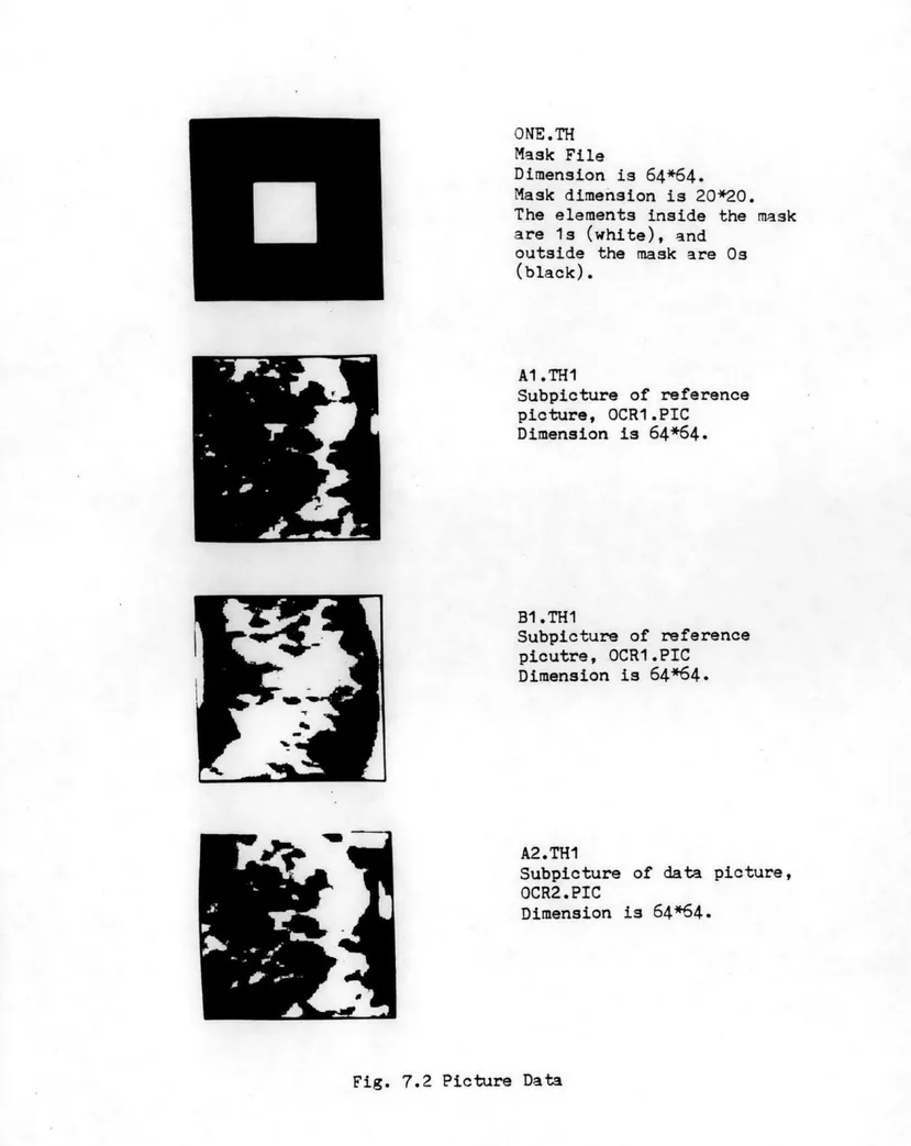
Some of the basic subpicture method algorithms are shown in Figure 2.3.1 and Figure 2.3.2. The reference picture OCR1.PIC and the data picture OCR2.PIC have the dimension of 256*256.

The operator identifies two subpictures, A1.PIC and B1.PIC, which are subtracted from the reference picture OCR1.PIC. The dimension of these

subpictures is 64*64 which enables short calculation time and FFT.

A region of interest which has 20*20 dimension is automatically defined by masking at the center of these subpictures, namely ROIA and ROIB. So, the operator must choose the x-y co-ordinates of these

subpictures so that a clear landmark should be at the center of the

subpicture and included in the 20*20 dimension of the region of interest. Two other subpictures, A2.PIC and B2.PIC, are subtracted from the data picture OCR2.PIC at the same x-y co-ordinates as Al.PIC and B1.PIC. Two regions of interest, ROIA and ROIB, and two subpictures, A2.PIC and B2.PIC, are Fourier transformed and filtered with Mexican hat filter. The filtering operation boosts the moderately high frequencies and

attenuates the low and very high frequencies. There are edge effects at the boundary of the image due to the filter. Therefore the outer three elements are masked to zero.

After being inverse Fourier transformed, ROIA is crosscorrelated with A2.PIC and ROIB is crosscorrelated with B2.PIC. The peak of each crosscorrelation is used as a measure of the translation of the region of interest between two subpictures.

The rotation angle calculation is simple.

( xal, yal

)

)

(

)

(

)

The inclination of the line which connects ( xal, yal

)

(

)

thetal=arctan((yal-ybl)/(xal-xbl))

The inclination of the line which connects ( xa2, ya2

)

(

)

theta2=arctan((ya2-yb2)/(xa2-xb2)) Therefore, the rotation angle is given by

Ln

N~

256

Subpicture

64

20

Region of Interest

ROIA

Subpicture

Subpicture

Subpicture

Fig. 2.3.1 Subpictures and Region of Interest

(x2a,y2a)

(xla,yla)

-Subpicture

(Xlb

Iylb)

(x2b,y2b)

Fig. 2.3.2 Crosscorrelation of Subpictures

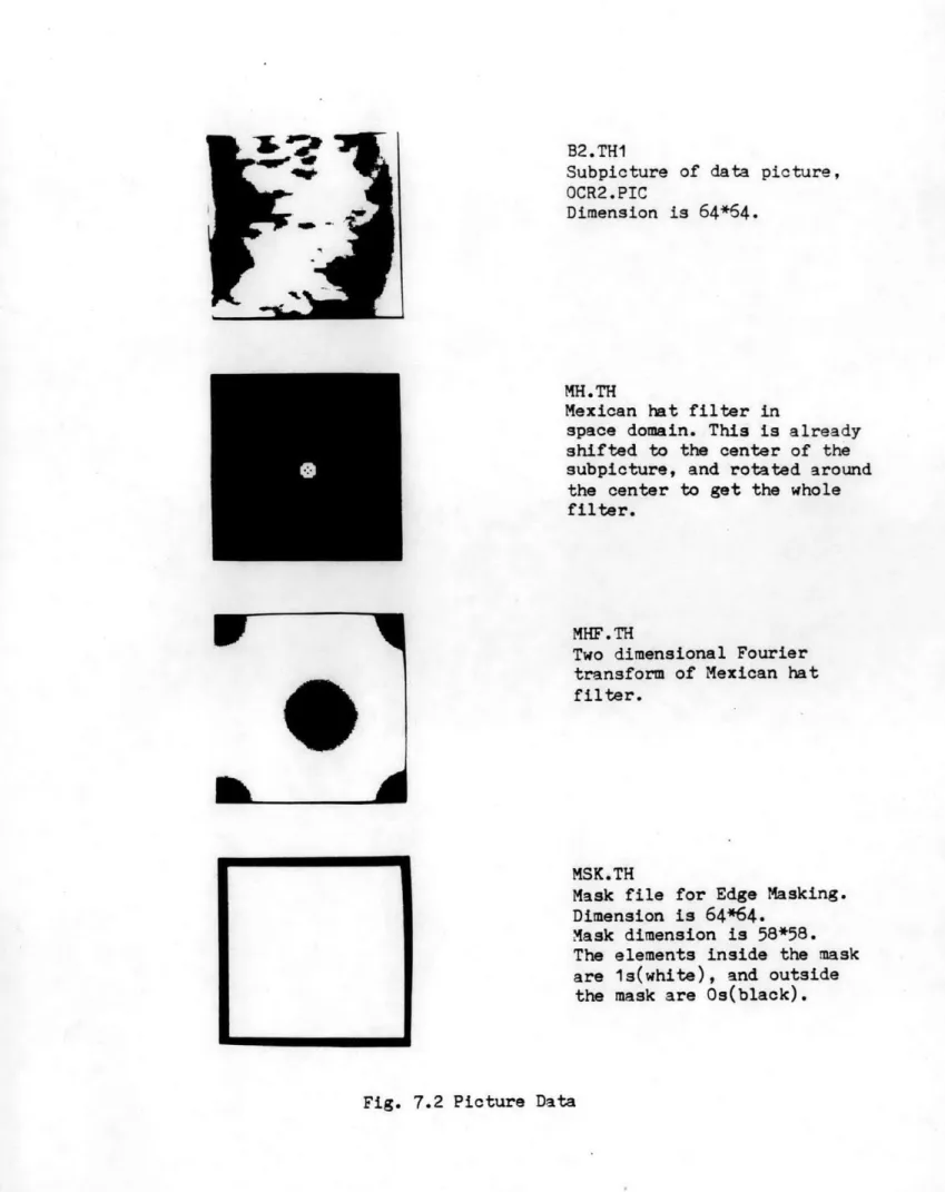
--3. Preconditionig of Image - Mexican Hat Filter

The human observer can measure the translation of an object on the x-y plane which is perpendicular to the line of sight, or on the video screen. So, if the visual signal process of humans is simulated by computer algorithm, it should be possible for software to measure the translation of an object on the video screen. A successful process was to use the Mexican hat filter ( Anthony Parker, 1983 ). Therefore, the same filter was used in this thesis.

This filter is the second derivative of a Gaussian function and given by

1/(sigma**2*sqrt(2*pi))*exp(-r**2/(2*sigma**2))

The name, Mexican hat, comes from the shape of this filter in the spacial domain.

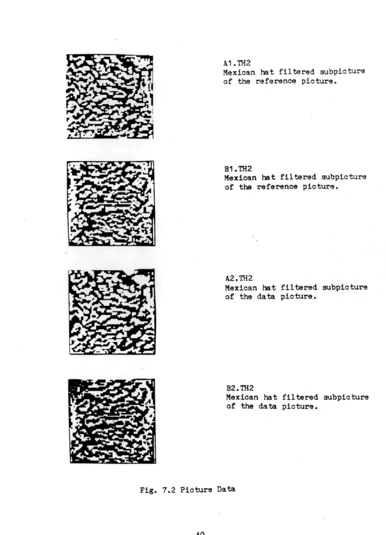
The effect of the Mexican hat filter is to boost the moderately high frequencies and reduces the magnitude of low frequency component and very high frequency component. Figure 7.2 MH.TH and MHF.TH shows the Mexican hat filter in position domain and frequency domain respectively. The filtering effect is shown in Figure 7.2 A1.TH2, B1.TH2, A2.TH2 and B2.TH2.

4. Extracting Torsion Measurement - Crosscorrelation

Crosscorrelation is a well known operation defined by Rflf2( i',j' )=sam(ij) ( fl( ij ) f2(*)( i-i',j-j

) )

fl( i,j ) is the first picture f2( i',j' ) is the second picture (*) is the conjugation operation

This crosscorrelation is normalized by the energy of the pictures R'f1f2( i',j' )=Rflf2( i',j' )/sqrt( eflef2

)

where

ef1 is the energy of the first image defined by efl=sum(i,j) ( f( ij ) f(*)( i,j ) )

ef2 is the energy of the second image defined by ef2=sum(i',j') ( f( i',j' ) f(*)( i',j' ) )

In this thesis, the normalization factor is calculated by

squaring the second image, multiplying the Fourier transform of the squared image by the transform of the mask, taking inverse Fourier transform and then taking the square root. The crosscorrelation and the normalization factor are shown in Figure 7.2 ONA.TH2 and ONB.TH2.

In this case, the image was filtered so as to increase the energy in the detail in the iris. For this reason, the peak in the

crosscorrolation funtion falls in a region where the energy is near the maximum. The peak is apparent even in the unnormalized crosscorrelation

₍

Anthony Parker 1983 ). When the peak is in a low energy region, it is often smaller than the side lobes. In that case, the normalization operation will make it possible to identify the peak when it could not otherwise be

identified.

But, if there is a strong reflection of any image on the iris, such as reflection of a rotating dome, it might be possible that there are two crosscorrelation peaks, one is for the eye image and the other is for the reflection movement. So, the image data should be as clear as possible.

5. Hardware Used to Inplement the Ocular Torsion Algorithm

5.1 Hardware of Man-Vehicle Laboratory

Figure 5.1 shows the computer system at the Man-Vehicle Laboratory, which is built around a Digital Equipment Corporation,

PDP-11/34 central processing unit with 256 kilobytes ( kB ) of main buffer memory, two 2.4 megabytes ( MB ) RK05 disk drives, a Microterm terminal ERGO 301, a WV-200P video camera, a NV-9300 video tape player, a WV-5300 video monitor and a Printronix MVP printer. The operating system used on this system is the RT-11 version 4.

The calculating power and speed are low because the buffer memory size is rather small and the system doesn't have an array processor. For

instance, 256*256 byte dimension of matrix data array or 64*64 complex dimension of matrix data array cannot be defined in the buffer memory. A

large program cannot be run and it was necessary that a large program must be divided into several parts. Two dimensional image data was manipulated every few rows of the image matrix and written in the disk memory with the record size of 128 ( 512 bytes ).

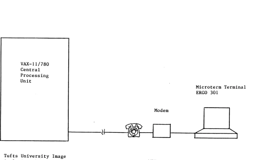
5.2 Hardware of Tufts University Image Analysis Laboratory

Figure 5.2 shows the hardware system of Tufts Image Analysys Laboratory computer system. The hardware system is VAX-11/780 with 4

mega-byte buffer memory, and the operating system is VMS Version 4.1. This system has the floating point accelerator.

System, because the calculation can be done in the buffer memory and doesn't need I/O operation between the buffer and the disc memory. While the program for RT-11 System needs 75 minutes to analyze an image, the program for VAX System needs only 2 minutes with I/O operation and only 30 seconds without I/O operation between the buffer and the disc memory.

Eye

WV-200P Video Camera

NV-9300 Video Tape Player

WV-5300 Video Monitor

Microterm Terminal ERGO 301

Printronix MVP Printer

Fig. 5.1 Computer System at Man-Vehicle Laboratory PDPll/34 Central

Processing Unit

c

VAX-i 1/780 Central Processing Unit Microterm Terminal ERGO 301 Modem

LZZZZ

IZ

Tufts University Image

Analysis Laboratory _{MIT Man-Vehicle Laboratory}

Fig. 5.2 Computer System at Image Analysis Laboratory rb.)

6. Data Format and Image Manipulation

6.1 Data Format

A frame grabber generates 256*256 dimension image data arrays. Each element is a byte which has 8 bit intensity capacity ( -127 to 127 ). An image can be taken from the video camera or the video tape player and displayed on the video monitor.

Image data is transformed from bytes into complex numbers by adding 0 element of the complex part for FFT and digital filtering.

6.2 Image Acquisition and Manipulation

The following commands are SET VD:CNTRL=0 SET VD:CLEAR=n*10 SET VD:SCROLL=n*10 SET VD:LEFT=n*10 SET VD:RIGHT=n*10 SET VD:TOP=n*10 SET VD:BOTTOM=n*10 SET VD:CNTRL=10000 R RUNAVE

useful for image manipulation. Reset the video screen

Set whole display equal to n*10 Load the scroll register

Set left bound of the screen at n*10 Set right bound of the screen at n*1 0

Set top bound of the screen at n*10 Set bottom bound of the screen at n*1 0

Connect the video monitor directly with the video camera or the video

tape player

the video frame grabber, multiple image had to be averaged to obtain a reasonable quality image. This command generates an averaged image on the video screen.

COPY VD:OCR1.PIC DAT: Copy the image on the video screen named OCRI.PIC into DAT: disk These commands can be refered in VDHELP.TXT in system disk of RT-11.

7. Software Description for RT-11 System

The programs for finding the image rotation are shown in Appendix 1. The used language for RT-11 System is RATFOR which can be preprocessed to standard Digital Equipment Corporation FORTRAN. A large program was divided into four parts; YOS11.RAT, YOS22.RAT, YOS3.RAT and YOS4.RAT. They were compiled with "/NOLINENUMBER" because of the small size of the central processor buffer memory.

YOS11.RAT is the main program for finding the image rotation angle. Input data files for this program are OCR1.PIC and OCR2.PIC. Output file is OCRBOX.DAT which includes the rotation angle of the pictures.

YOS22.RAT, YOS3.RAT and YOS4.RAT are the programs of subroutines which must be linked to the mainprogram.

7.1 YOS11.RAT

YOS11.RAT is the main program for finding the image rotation angle. The data flow chart is shown in Figure 7.1. Picture data are shown

in Figure 7.2. Input data files for this program are OCR1.PIC ( a reference picture ) and OCR2.PIC ( a data picture ) stored in logical unit DAT:. These files are 256*256 bite dimension raw pictures. The data files manipulated in this program are filed in the disc memory of the computer evey time when they are created or manipulated by subroutines because of

the rather small size of the buffer memory with the recordsize 128 ( 512

bytes ). This makes the calculation time so long as 75 minutes.

the subroutine "pdb". The picture descriptor block is 512 bytes and has the information of the picture file such as the dimension of the picture, the maximum value of the picture elements and the x-y coordinates of the

subpicture. The new files to which the picture descriptor block is added are OCR1.PDB and OCR2.PDB.

Subroutine "box" is called to define the x-y coordinates of the subpictures A1.PIC and B1.PIC. The operater can see the subpictures on the video screen. The x-y coordinate data is stored in the data file A.DAT for the subpicture A1.PIC and in the data file B.DAT for the subpicture B1.PIC by the subroutines "bopenf" to open the files and "rput" to store the data.

Mask file defines the region of interest and stored in file

ONE.Z. This file is created by the subroutine "maksr". The dimension of the mask ( 64*64 ) must be the same as the subpictures. The intensity of the elements inside the mask is 1 and the intesity outside the mask is 0. Masking routine is that if the element of the mask is 0, the corresponding element of the output subpicture element is also 0. The location of the mask is the center of the subpicture ( 32,32 ). The size of the mask is ( 20*20 ). Therefore, the operater must choose the subpictures so that the subpictures may include a clear landmark of the iris.

OCR1.PDB and OCR2.PDB are transformed into complex value format by adding zero element of the imaginary part of the data by the subroutine

"czcvt" so that Fourier transform and filtering can be done. From this part of the program, the picture data is manipulated in complex format.

Four subpictures are taken using x-y coordinates data, A.DAT and B.DAT. The names of the subpictures are A1.Z and B1.Z for the reference picture, and A2.Z and B2.Z for the data picture. Each element of these

Subroutine "masr8" is called to create the Mexican hat filter. This subroutine only creates 1/4 of the whole filter on the subpictures. The filter must be shifted at the center of the subpicture and rotated,

because the filter is created only in the area where x-y coordinates are positive. Subroutine "rot11" rotates the filter and create the whole filter

in the space domain.

Mexican hat filter is Fourier transformed by the subroutine "xform option 'FFT'". The file name is MHF.Z. The subpictures A1.Z, B1.Z, A2.Z and B2.Z are also Fourier transformed by the same subroutine and filtered with MHF.Z. Filtering operation is done by multiplying each element of the Fourier transform of subpictures by the element of the filter.

Subroutine "xform optiton 'Inverse FFT'" is called to inverse Fourier transform the subpictures A1.Z, B1.Z, A2.Z and B2.Z and edge masked by the edge mask MSK.Z. This mask file is created by the subroutine

"maksr", and all three elements of the subpictures are masked. The masking operation is the same as the filtering operation, that is the muliplication of the each element of the mask and the subpictures. This is the end of the Mexican hat filtering operation.

Following is the crosscorrelation routine. The algorithm of this routine is explained in the section 4.

A2.Z and B2.Z are normalized and masked by the subroutine "normf" and squared by the subroutines "copy" and "twofil (option multiplication)". The masking file name is ONE.Z. The squared data subpictures are AA2.Z and BB2.Z. All these files, A2.Z, B2.Z, AA2.Z and BB2.Z, are Fourier

transformed by the subroutine "xform (option FFT)".

complex conjugates of A1.Z1 and B1.Z1. AA2.Z and BB2.Z are also multiplied by the complex conjugates of ONE.Z1 and ONE.Z2. Rsulting data files are ONE.Z1 and ONE.Z2. A1.Z1, B1.Z1, ONE.Z1 and ONE.Z2 are inverse Fourier

transformed. The square root files of ONE.Z1 and ONE.Z2 are taken by the subroutine "onefl9". A1.Z1 and B1.Z1 are divided by ONE.Z1 and ONE.Z2 respectively. Rsulting files, A1.Z1 and B1.Z1, are the crosscorrelation functions. The square root of these files, ONE.Z1 and ONE.Z2, are the normalization factors. Detail explanation of the normalization factor is given in section 7.2.

Two final crosscorrelation functions, A1.Z1 and B1.Z1, are used to find the peak of the correlation and the translation of the region of interest by the subroutine "peak4". The actual rotation angle is calculated by the subroutine "calc20" and the data are stored in the file OCRBOX.DAT.

7.2 YOS22.RAT

YOS22.RAT is composed of main subroutines which are called by the main program YOS11.RAT. Basically, these main subroutines open files and the calculation data are stored in the files because of the small size of

the buffer. 128 of recordsize ( 512 bytes ) is used for I/0. This causes the calculation time to be slow.

subroutine pdb(cstrl,cstr2)

The subroutine pdb puts the picture descriptor block ( 512 bytes

)

in the fifteenth block and vertical dimension is stored in the sixteenth block.

subroutine maksr(cstr,iszx,iszyrmag,xO,yO,xc,yc)

This subroutine makes a mask file. The mask file is like a

window. Each element inside the window has the value of " rmag " ( usually rmag=1.0 ), while the elements outside the window are zero's such as

zline(ix)=zmag else

zline(ix)=(0.,O.)

The center of the window is ( xc,yc ). The size of the window is (2*xO)*(2*yO). ( iszx,iszy ) must be the same as the dimension of the subpicture which is to be masked ( 64*64 ). The window defines the region of interest in the subpictures. "cstr" is the mask file name such as MSK.Z or ONE.Z. Subroutine "ouplnz" is called to file the mask data into the disc memory line by line of the mask file elements.

subroutine subpic(cstrl,cstr2,cstr3,iszx2,iszy2)

This subroutine makes a subpicture file whose dimension is ( iszx2*iszy2 ). In this thesis, the dimension is ( 64*64 ). The x-y coordinates data of the subpicture are stored in the file " cstr3 ". "

cstr2 " is the subpicture file name taken from the original picture " cstrl ". This program also puts the maximum value of the picture elements and the x-y coordinates of the subpicture as x-offset and y-offset in the picture descriptor block. The value of x-y offset is used by the subroutine "

calc20 " for calculating the rotation angle.

subroutine maksr8(cstr,iszx,iszyrmag,xO,yO,sigma)

This subroutine makes the Mexican hat filter centered at the upper left corner ( 0.0 ). Therefore, this filter must be shifted at the center of the subpicture and rotated. The value of the filter in the space domain is given by

zline(ix)=sigma_4_2_pi inverse*(2.-varinverse*rsq)*

exp(-twovar inverse*rsq) + i*0. (i=root(-1)) [ zline( ix)=cmplx(sigma_4_2_pi-inverse*(2.-varinverse*rsq)* exp(-twovarinverse*rsq),0.) ] where sigma_4_2_piinverse=1./(sigma**4*sqrt(2.*pi)) twovarinverse=1./(2.*sigma**2) varinverse=1./sigma**2

Subroutine "ouplnz" is called to file the Mexican hat filter into the disc memory line by line of the filter elements.

subroutine rot11(cstr1,cstr2,ix,iy)

This subroutine shifts the Mexican hat filter, " cstrl ", created by the subroutine maksr8 to ( ix,iy ) and rotates it around the center of the subpicture, since the filter file which is created by the subroutine "maksr" is only 1/4 of the whole filter at the upper left corner of the subpicture. The statement for the rotation is

The data of "zline2" is written by the subroutine "ouplnz" line by line. The new file " cstr2 " is the Mexican hat centered at ( ix,iy ).

subroutine xform(iop,cstr)

This subroutine does the two dimensional discrete Fourier

transform. " iop=10 " is Fourier transform. " iop=11 " is inverse Fourier transform. Transformation is done row by row of the image data matrix by the subroutine "fft", and the matrix is transposed by the subroutine "transp". Fourier transform is done row by row again for two dimension. Another matrix transpose may be taken. But, in this subroutine, it is eliminated for saving time.

subroutine twofil(cstr1,cstr2,iop,rmin)

This subroutine operates multiplication of the two files, " cstrl " and " cstr2 " such as

zrec2(i)=zrecl(i)*zrec2(i)

and multiplication of " cstrl " by the conjugate of the file " cstr2 " _such as

zrec2(i)=zrecl(i)*conjg(zrec2(i))

and division of the file " cstrl " by " cstr2 ". The operation is done picture element by element. In order to avoid zero-divide, the minimum value of the second file elements is defined by " rmin ", that is

if(abs(real(zrec1(i))).ge.rmin)

zrec2(i)=real(zrec2(i))/real(zrec1(i)) + i*0. (i=root(-1)) [ zrec2(i)=cmplx(real(zrec2(i))/real(zrecl(i)),o.) ]

else

zrec2(i)=(O.,O.) where

zrecl(i) is an element of the file "cstrl" zrec2(i) is an element of the file "cstr2".

subroutine normf(cstrl,cstr2)

This subroutine is used for creating a picture file of the region of interest from the mask file " cstrl " and the subpicture file " cstr2 ". At the first part of this program, mean value of the subpicture elements "

zmean " and the normalization factor " rootsq inverse " are calculated. 1.

rootsq_inverse=

Vsumsq-abs (z sum) /npel

[

I

sumsq is the sum of the absolute value of all picture elements. zsum is the sum of the all picture elements.

" npel " is the number of the picture elements ( 64*64=4096 ).

If the picture element of the mask file is zero, the element of the output file is also zero, which means the masking. If the picture element of the mask file is not zero, the element of the subpicture is normalized by "

rootsqinverse ".

This subroutine takes the square root of the real part of the picture element by the statement

zrecl (i)= Vmzax (O. , real (zrecl (i)) + i*0. (i=root (-1))

[ zrec1(i)=cmplx(sqrt(amax1(O.,real(zrec1(i)))),o.) ] where zrecl(i) is an element of the subpicture data file.

If the real part is negative, the result is set to zero in the output file.

subroutine peak4(cstrl,cstr2,n)

This subroutine calculates the x-y coordinates of the correlation peak, ( rx,ry ) from the crosscorrelation function " cstrl ". The peak position is interpolated between the peak element and the next element by the high resolution cubic spline. This function was used successfully by Anthony Parker (1983), so the same function is used in this subroutine. Interpolation is " tOx,tOy ". tOx=tO(temp(1),temp(2) ,temp(3)) where temp(i)=f of t(tOy,f(i,1),f(i,2),f(i,3)) tO(flf2,f3)=(f1-f3)/(2.*(f1-2.*f2+f3)) f_oft(tO,f1,f2,f3)=(f1-2.*f2+f3)/2.*tO**2+(f3-f1)/2.*tO+f2 f(i,j) is the element of the crosscorrelation function. and

tOy=tO(temp(1 ) ,temp(2) ,temp(3)) where

temp(i)=f of t(tx,f(1,i),f(2,1),f(3,1))

f_of_t(tOf1,f2,f3)=(f1-2.*f2+f3)/2.*tO**2+(f3-f1)/2.*tO+f2 f(i,j) is the element of the crosscorrelation function.

The subpicture location in the reference picture is stored in the picture descriptor block and is read in this program ( xoffsetyoffset ). The correlation peak location is the sum of these values.

peak location=( xoffset+rx+tOx , yoffset+ry+tOy

)

subroutine calc20(cstr,nl,n2,n3)

This subroutine calculates the rotation angle from the two

correlation peak positions ( x2a,y2a ) and ( x2b,y2b ), and two subpicture locations ( x1a,y1a ) and ( x1b,y1b ).

HESOT. TXT

*h asi 1at, explanat;on Rev Non Nagashima f.~ 4 4. 4* Id - c- a -. :- .It INPUT pNP1jT 1 TIC EREFERENCE PICTUPE,

ADD PICTURE DESCRIPTER DLOCK OCR1. PDB A.DAT(DEFINE SUB PICTURE A LOCATION) B.DAT(DEFINE SUB PICTURE B LOCATION)

ONE. Z(MAKE MASK FILE (64*64)

(REGION OF INTEREST ALSO DEFINED)

0CR2. PLG

(DATA

ADD PICTJRE DESCRIP TER

BLOCK OCR2. PDB

(ONE. TH) IS

DATA TRANSLATE INTO COMPLEX NUMBER DATA TRANSLATE NUMBER INTO COMPLEX OCR 1, Z +---OCR2. Z ---*A. DAT

MAKE SUB PIC Al. Z(Al. THI)

(64*64) E C C

*

c

MAKE SUB PIC B1 Z(Bl. THl)

k64*64)

*A. DAT

MAKE SUB PIC A2. Z(A2. THI)

(64*64)

*B. DAT

MAKE SUB PIC 32. Z(B2. TH1) (64*64)

MH. Z(MAKE MEXICAN HAT FILTER) (MH. TH) FFT

MHF. Z(MHF.TH)

MSK.Z(MAKE EDGE MASK OF MEXICAN HAT FILTER)(MSK.TH) .1 2 2 I I

FFT OF SUBPIC Al. Z *MHF. Z MEXICAN HAT FILTER Al. Z FFTC-1J OF SUB PICTURE Al. Z(AI. TH2) *MSK. Z EDGE MASKING Al. Z *ONE. Z MAKE REGION OF INTEREST A .Z(Al. TH3) FFT OF SUBPIC D1. Z *MHF. Z MEXICAN HAT FILTER 91 z FFTC-13 OF SUB PICTURE 81. Z(B1. TH2) *MSK. Z EDGE MASKING 81. Z *ONE. Z MAKE REGION OF INTEREST 31. Z(81. TH3) FFT OF SUBPIC A2. Z *MHF. Z MEXICAN HAT FILTER A2. Z FFTC-13 OF SUB PICTURE A2. Z(A2. TH2) *MSK. Z EDGE MASKING A2. Z FFT QF SUBPI : B2. Z *MHF. Z MEXICAN HAT FILTER B2. Z FFTC-13 OF SUBPICTURE 32. Z3(B2. TP42) *MSK. Z EDGE MASKING B2. Z *-COPY--A2. Z FFT A2. Z + +-COPY--+ AA2. Z H2. Z [B2. Z A2. Z 9 .2.? SQUARE SQUARE AA2. Z (AA2. TH) FFT AA2 z 132. BB2. Z (1302

TH1'

81. ZI ONE. Z1- -COPY-ONE. Z2 CONJG +---) CONJG ( - - - )'( --- ONE. Z1* ONE. Z1 ( ---

)

ONE. Z1(ONA. THI) ONE -- ; '. SQUARE ROOT SQUARE IR

ONE. Z1(ONA. TH2) ONE 2i *1/ONE.Zl<---)

Fig. 7.1 Data Flow Chart

OCR1.PIC

Reference Picture and Two Subpictures

OCR2.PIC Data Picture

ONE.TH Mask File

Dimension is 64*64. Mask dimension is 20*20. The elements inside the mask are 1s (white), and

outside the mask are Os (black). A1.THI Subpicture of reference picture, OCR1.PIC Dimension is 64*64. B1.TH1 Subpicture of reference picutre, OCR1.PIC Dimension is 64*64. A2.THI

Subpicture of data picture, OCR2.PIC

Dimension is 64*64.

B2.TH1

Subpicture of data picture, OCR2.PIC

Dimension is 64*64.

MH.TH

Mexican hat filter in

space domain. This is already shifted to the center of the subpicture, and rotated around

the center to get the whole filter.

MHF. TH

Two dimensional Fourier transform of Mexican hat filter.

MSK.TH

Mask file for Edge Masking. Dimension is 64*64.

Mask dimension is 58*58.

The elements inside the mask

are ls(white), and outside

the mask are Os(black).

Fig. 7.2 Picture Data Pk Mk

161 42W

"Wro W hL

dm6

J

B2. TH2

Mexican hat filtered subpicture of the data picture.

Fig. 7.2 Picture Data Al .TH2

Mexican hat filtered subpicture of the reference picture.

B1 .TH2

Mexican hat filtered subpicture of the reference picture.

A2.TH2

Mexican hat filtered subpicture of the data picture.

Al .TH3

Region of interest.

This is the multiplication of the two files, the reference subpicture A (already filtered) and the mask file.

The dimension of the region of interest is 20*20.

B1.TH3

Region of interest.

This is the multiplication of the two files, the reference subpicture B (already filtered) and the mask file.

The dimension of the region of interest is 20*20.

AA2.THI

Square of A2.TH

This is used to get the crosscorrelation function.

BB2.TH1

Square of B2.TH

This is used to get the crosscorrelation function.

ONA.TH1

This is the multiplication of the conjugate of mask file and AA2.TH1, and used to get the normalization factor.

ONB.TH1

This is the multiplication of the conjugate of mask file and BB2.THI, and used to get the normalization factor.

ONA.TH2

Square root of ONA.TH1 This is the normalization factor.

ONB.TH2

Square root of ONB.TH1 This is the normalization factor.

Fig. 7.2 Picture Data

8. Software Description for VAX System

The programs for finding the image rotation are shown in Appendix 2. The used language is RATFOR and the programs are compiled by RT-11

RATFOR compiler to FORTRAN, since Tufts VAX System doesn't have a RATFOR compiler.

The program is composed of four parts: YTFS1.FOR, YTFS2.FOR, YTFS3.FOR and YTFS4.FOR. The algorithm of the calculation is the same as

the software for RT-11 System. But the image data manipulation is done in the buffer memory defining image data matrices, which enabled the program to be simple and calculation time to be short. This is the advantage of using the VAX System.

YTFS1.FOR defines subpicture location. YTFS2.FOR creates several picture files from the reference picture OCR1.PIC, which are necessary to use the main program. YTFS3.FOR is the main program for analyzing the image rotation. YTFS4.FOR is the program of subroutines which must be linked to the other programs.

8.1 YTFS1.FOR

This program defines subpicture location. At first, the operator must get a reference picture on the video screen and run this program. Subroutine "box" is called to define the x-y coodinates of the two

subpictres, A.PIC and B.PIC. Subpicture dimension ( 64*64 ) is also defined in this program. The x-y coordinates data are stored in the files A.DAT for the subpicture A1.PIC and B.DAT for the subpicture B1.PIC. This program must be run in RT-11 System at the Man-Vehicle Laboratory and the data

files must be transfered to the VAX System at Tufts University Image Analysis Laboratory.

8.2 YTFS2.FOR

This program creates several picture files from the reference picture OCR1.PIC, which are necessary to analyze the data picture OCR2.PIC using the program YTFS3.FOR. Inputs are the files of reference picture and x-y coordinates of subpictures, A.DAT and B.DAT. Output files are complex value transformed subpictures, A1.Z and B1.Z, a mask file, ONE.Z, which defines the region of interest in the subpictures, Fourier transform of Mexican hat filter, MHF.Z, and MSK.Z which is an edge masking file. These two dimensional data array matrices, ONEZ,A1Z,B1Z,MHZ,MHFZ,MSKZ, can be defined in the large buffer memory of the VAX System. This enables the very short analyzing time which was impossible for the RT-11 system of the

Man-Vehicle Laboratory.

Subroutine "ymaksr" is called to create the mask file, ONE.Z. Dimension of this mask ( 64*64 ) must be the same as the subpictrues and defined by this calling routine. Magnitude of the mask, which is the

magnitude of each picture element of this data file, is 1 so that there is not any change of the intensity of the data pictures. Dimension of the mask is also defined here and it is 20*20. The location of the mask is ( 32,32

)

which is the center of the subpicture. Therefore, the dimension of the region of interest is 20*20 and the location is the center of the

subpictures. The operater should choose the subpicture location so that the region of interest includes a clear landmark of the iris.

and B.PIC. This subroutine opens the data files of the x-y coordinates of the subpictures, A.DAT and B.DAT, and the reference picture, OCR1.PIC. A.PIC is created from OCR1.PIC using the coordinates A.DAT, and B.PIC is created from OCR1.PIC using the coordinates B.DAT. Subpicture data array matrices, A1Z and B1Z, are defined in the buffer memory of the computer.

Subroutine "ymksr8" is called to create the Mexican hat filter, MHZ. The dimension of the filter ( 64*64 ) must be the same as the

subpictures. As the filter is created at the upper left corner, it must be shifted to the center of the subpicture. The shifting amount is ( 32,32

).

Subroutine "yrot11" is called to rotate the filter around the center of the file ( 32,32 ), since the filter created by the subroutine "ymksr8" is 1/4 of the whole filter on the subpictures. The new data array matrix name is MHFZ.

Subroutine "yxform" is called to Fourier tramsfrom the Mexican hat filter MHFZ.

Subroutine "ykeep" is called to store the data array MHFZ in the data file MHF.Z. This is necessary because MHF.Z is used by YTFS3.FOR.

Subroutine "ymaksr" is called to create the edge mask array matrix MSKZ. The dimension of the edge mask is the same as the Mexican hat

fiter. Intensity of the elements is 1 as well as the mask file MHK.Z. The location of the mask is the center of the filter ( 32,32 ) and all three elements of the edge are masked.

Subroutine "ykeep" is called to store the data array matrix MSKZ in the data file MSK.Z. This is necessary because MSK.Z is used by

YTFS3.FOR.

Subroutine "yxform" is called to Fourier transform the subpicture data array matrices, A1Z and B1Z, which are already defined in the buffer

memory of the computer.

Subroutine "y2fil" is called to filter the subpicture data array matrices, A1Z and B1Z, with the Mexican hat filter data array matrix, MHFZ. The filtering routine is done by multiplying each picture element by the

data element of the filter.

The data array matrices, A1Z and B1Z, are inverse Fourier

tranformed for the edge masking by the subroutine "yxform ( option FFT[-1] )" and multiplied by the edge masking array matrix, MSKZ, by the subroutine "y2fil ( option multiplication )".

Subroutine "ynormf" is called to create the region of interest data array matrices, A1Z and B1Z, using the mask file array matrix, ONEZ. This routine is done by multiplying each subpicture element by the mask

leement. Inside the region of interest, the intensity of each element of the mask is 1, and the intensity outside the region of interest is 0. The masking routine is that if the mask element is 0, the output matrix element

is also 0. Each output element is normalized by the normalization factor. Detail explanation is given in section 8.4.

Region of interest data array matrices, A1Z and B1Z, and mask array matrix, ONEZ, are stored in the data files, A1.Z, B1.Z and ONE.Z, so that they can be used by other main programs such as YTFS3.FOR.

8.3 YTFS3.FOR

This is the main program for analyzing the image rotation using several data files created by YTFS2.FOR.

Input data files are OCR2.PIC which is 256*256 byte dimension raw image data file, A1.Z and B1.Z, which are the subpictures of the reference

picture, A.DAT, B.DAT, MHF.Z and MSK.Z. The rotation angle data are stored in the output file OCRBOX.DAT.

The two dimensional data array matrices, A2ZB2ZMHFZ,MSKZ,AA2Z, BB2Z,ONEZ1,ONEZ2,A1Z1,B1Z1, can be defined in the large buffer memory of

the VAX system. This enables the simple composition of the programs and the very short analyzing time for analysis because I/O operation between the buffer and the disc memory is not necessary, which was not possible for the RT-11 system of the Man-Vehicle Laboratory. The calculation takes 75

minutes for RT-11 System and only 30 seconds for VAX System to analyze an image.

Subroutine "ysbpic" is called to create the subpicture array matrices, A2Z and B2Z, form the data picture file, OCR2.PIC, which is

opened by this subroutine. X-Y coordinate data files, A.DAT and B.DAT, are also opened by this subroutine and used for creating the subpicture data matrices.

Subpicture array matrices, A2Z and B2Z, are Fourier transfromed by the subroutine "yxform ( option FFT )" for filtering.

Subroutine "filbuf" gets the Mexican hat filter data file and defines it as a two dimensional data array matrix, named MHFZ, in the buffer memory.

The subpicture data array matrices, AZ2 and B2Z, are multiplied, element by element, by the filter array matrirx, MHFZ, which is defined in the buffer memory by the subroutine "filbuf" from the filter data file, MHF.Z. This is the Mexican hat filtering operation.

After the filtering, subpicture matrices, A2Z and B2Z, are inverse Fourier transfromed by the subroutine "yxform ( option FFT[-1] )" and edge masked. The edge masking operation is also the multiplication of

the subpicture data array matrix and the edge masking data array matrix, MSKZ, element by element. This is the end of the Mexican hat operation.

The following is the crosscorrelation operation. The algorithm of the crosscorrelation is explained in the section 4.

Subroutine "copy" is called to create the same subpicture data array matrices in the buffer memory in order to get the energy of the

pictures. A2Z and B2Z are copyed in the array matrices, AA2Z and BB2Z, respectively. A2Z and AA2Z, and ,B2Z and BB2Z, are multiplied respectively to get the square value of the subpictures and Fourier transformed before the crosscorrelation.

Subroutine "filbuf" is called to get the subpicture data files of the reference picture, A1.Z and B1.Z, and defines the array matrices, A1Z1 and B1Z1, in the buffer. Complex conjugate matrices of the A1Z1 and B1Z1 are multiplied by the data subpicture matrices, A2Z and B2Z.

On the other hand, spuare value matrices of the data subpictures, AA2Z and BB2Z, are multiplied by the conjugate matrices of the mask file, ONEZ1 and ONEZ2, which are the same at this time. Resulting array matrices are ONEZ1 and ONEZ2. These array matrices, A1Z1,B1Z1,ONEZ1,ONEZ2, are

inverse Fourier transformed. Square root matrices of ONEZ1 and ONEZ2 are taken, and A1Z1/ONEZ1 and B1Z1/ONEZ2 are the crosscorrelation functions. These operations such as the multiplication and the division are the

calculation of element by element of the array matrices. This is the end of the crosscorrelation operation. Resulting crosscorrelation functions are A1Z1 for the subpicture A2.PIC and B1Z1 for the subpicture B2.PIC.

Subroutine "ypeak4" is called to identify the crosscorrelation peak of the function. The peak coordinates of A1Z1 and B1Z1 are ( x2a,y2a

)

Therefore the coordinates of the subpictures are also necessary to get the peak location on the original 256*256 dimension coordinates.

Subroutine "datatr" transfers the data from the data files, A.DAT and B.DAT into the buffer, and gets the x-y coordinates data of the

subpictures on the original picture matrix ( 256*256 ) into the buffer. Subroutine "yclc20" calculates the actual rotation angle using the x-y coordinates of the subpictures on the original 256*256 matrix ( (x1a,y1a) and (x2b,y2b) ) and the crosscorrelation peak locations on the subpicture 64*64 matrices ( (x2a,y2a) and (x2b,y2b) ). Calculation

algorithm is

angle=arctan( yla-ylb,xla-xlb

)

)

The rotation angle data is stored in the file OCRBOX.DAT.

8.4 YTFS4.FOR

This is the program of subroutines which are used by the main programs YTFS1.FOR, YTFS2.FOR and YTFS3.FOR. All of the data arrays

manipulated in the subroutines are defined as two dimensional matrices of complex value. The data manipulation is done in the buffer memory of the computer and I/O operations are avoided as many as possible. Large buffer memory of the VAX system enabled these and very fast analyzing time and simple programs.

subroutine ymaksr(zsubiszxiszyrmagixO,iyO,ixc,iyc)

The subroutine "ymaksr" creates a rectangle mask in the buffer memory for making the region of interest or the edge masking file. "zsub"

is the name of the created mask such as ONEZ or MSKZ. "iszx" and "iszy" are the dimension of the mask data array matrix ( 64*64 ) which is the same as the subpictures. "rmag" is the magnitude of the mask inside the region of interest or the edge mask, and usually this is 1 so that there is not change of the intensity of the data files. "ixO" and "iyO" are the half size of the region of interest or the edge mask. "ixc" and "iyc" are the

x-y coordinates of the center of the mask on the subpicture matrix. Mask creating operation is

zsub(i,j)=1. inside the mask

zsub(i,j)=O. outside the mask

where zsub(ij) is an element of the mask array matrix.

subroutine ysbpic(zsubcstrl,cstr2)

This subroutine creates a subpicture array matrix in the buffer memory. "zsub" is the name of the subpicture array matrix such as A1Z or B1Z. "cstrl" is the name of the picture data file whose dimension is 256*256 byte dimension ( not the complex value ) such as OCR1.PIC or

OCR2.PIC. "cstr2" is the file name of the x-y coordinates of the subpicture such as A.DAT or B.DAT.

Subroutine "bopenf" is called to open the file of the x-y

coordinates of the subpicture center. The x-y coordinates data ( xO,yO ) is stored in the buffer memory by the subroutine "rget". Since these value are the center position of the subpicture on the matrix, the x-y coordinates of the upper left corner are necessary to create the subpicture, such as

ixO=xO-32. iyO=yO-32.

read. But the recordsize of the picture file is 128, therefore only 512 bytes data is read. In this program, the matrix data array cpic(ii,jj) whose dimension is 256*256 byte is defined, so that the program is very

much understandable. Each element of the matrix cpic(ii,jj) is a byte. The matrix csub(k,l) is defined as the subpicture data array matrix whose dimension is 64*64 and each element of the matrix is still a byte.

The last routine of this subroutine is the byte-complex convert. Byte is converted into the integer value by the following statements.

equivalence (c,ic) ! c and ic are equivalent

data ic// ! clear high byte

c=csub(i,j) isub(i,j)=ic

The integer value matrix is converted into a complex value matrix by adding a complex zero element to each real part of the data such as

zsub(i,j)=cmplx(float(isub(i,j)),O.)

where zsub(i,j) is the 64*64 complex dimension subpicture data array matrix.

subroutine ymksr8(zsub,iszx,iszy,rmag,xO,yO,sigma)

This subroutine is to create the Mexican hat filter matrix in the buffer. "zsub" is the name of the filter, iszx and iszy are the dimension of the filter which must be the same as the subpictures such as 64*64,rmag is a dummy variable,xO and yO are the center location of the filter and

sigma is the standard deviation. The created filter is centered at the upper left corner (0,0). Therefore, this filter must be shifted at the

center of the subpicture and rotated. The value of the filter in the space domain is given by

zsub(i,j )=sigma_4_2_pi inverse*(2. -varinverse*rsq)*

exp(-twovar inverse*rsq) + i*O. (i=root(-1))

[

(2.-varinverse*rsq)*exp(-twovar inverse*rsq) ,O.)

]

var inverse=1./sigma**2

twovarinverse=1./(2.*sigma**2)

sigma_4_2_pi_inverse=1./(sigma**4*sqrt(2.*pi))

subroutine yrotl1(zsubl,zsub2,ix1,iyl)

This subroutine is to rotate the Mexican hat filter around the center of the matrix by the following statement.

zsub2(i,(mod(j-1+ix,64)+1))=zsubl(i,j) where

zsubl(i,j) is the original Mexican hat filter zsub2(i,j) is the rotated Mexican hat filter

Fourier transform is still necessary for the filtering.

subroutine yxform(iop,zsub)

This program is to two dimensional Fourier transfrom if the option number iop is 10, and is to two dimensional inverse Fourier

transfrom if the option number is not 10. "zsub" is the data array matrix name which is to transformed.

zline(j) is defined by each row of the matrix zsub(i,j) and the subroutine "fft" operates the Fourier transform row by row. Subroutine "lytrnsp" is called to get the matrix transpose by the routine such as

zsub(i,j)=zsub(j, i)

and subroutine "fft" is called again and operated row by row for the two dimensional FFT. The matrix transpose may be taken again, but in this program, it is ignored for saving the calculation time.

subroutine y2fil(zsubl,zsub2,iop,rmin)

This subroutine is to operate multiplication, conjugate

multiplication and division element by element of the picture array matrix whose dimension is 64*64.

The option number, iop, 20 is for the multiplication by the following statement.

zsub2(i,j)=zsubl (i,j)*zsub2(i,j)

The option number 21 is for the conjugate multiplication by the following statement.

zsub2(i,j)=zsubl(i,j)*conjg(zsub2(i,j))

The option number 23 is for the division by the following

statement.

zsub2(i,j)=cmplx(real(zsub2(i,j))/real(zsubl(i,j)),0.)

If the real part of zsubl(i,j) is smaller than rminl, zsub2(i,j)=(0.,0) to avoid the overflow.

where rminl=rmin*"maximum absolute value of the real part of zsub2(i,j)"

This subroutine is to create the array matrix of the region of interest from the mask data matrix zsubl and the subpicture data matrix zsub2. At the first part of this subroutine, mean value of the subpicture elements "zmean" and the normalization factor "rootsqjinverse" are

calculated such as

1.

rootsq-inverse=

rn sumsq-abs (z sum) /npel

[

]

tsumsq" is the sum of the absolute value of all picture elements of zsub2(i,j).

"zsum" is the sum of the all picture elements of zsub2(i,j). "npel" is the number of the picture elements ( 64*64=4096 ). If the picture element of the mask matrix is zero, the element of the output matrix is also zero, which means the masking. If the picture element of the mask array is not zero, the each element of the subpicture matrix is normalized by "rootsq inverse" such as

zsub2(i,j)=(zsub2(i,j)-zmean)*rootsq inverse

subroutine yl fil( zsub)

This subroutine is to get the square root of each element of the data matrix zsub(i,j) by the following statement.

zsub(i,j)=cmplx(sqrt(amaxl(O.,real(zsub(i,j)))),0.)

This subroutine calculates the x-y coordinates of the correlation peak (x,y), from the crosscorrelation function zsub(i,j). The peak position is interpolated between the peak element and the next element by the

following interpolation operations. tOx=tO(temp(1),temp(2) ,temp(3)) where temp(j)=foft(tOy,f(j,1),f(j,2),f(j,3)) f of t(to,f1,f2,f3)=(f1-f3)/(2.*(f1-2.*f2+f3)) dimension f(3,3),temp(3) and tOy=tO(temp(1),temp(2) ,temp(3)) where

temp( j)=foft( tOx, f(1 , j) ,f (2, j) , f(3 , j))

f_oft(tO,f1,f2,f3)=(f1-f3)/(2.*(f1-2.*f2+f3)) dimension f(3,3),temp(3) and where f(j,i)=real(zsub2(i,jj)) jj=mod(x+(j-2)+63,64)+1 zsub2(i,j)=zsub(mod(y+i-2+63,64)+1,j)

zsub(i,j) is the element of the crosscorrelation function. (tOx,tOy) is the interpolation. (x,y) is the peak location of the

croSscorrelation function. Therefore, calculated peak location is (x+tOx, y+tOy) on the subpicture coordinates. This is the high resolution cubic spline used by Anthony Parker (1983) successfully and the same function is used in this subroutine.